Downloaded 159 times

![6
How did we get here?
Base rate Prediction for John
22%
𝑓 𝑥0
16%
𝐸[𝑓 𝑋 ]](https://image.slidesharecdn.com/1140amgpscottlundbergfinalv2-191022184911/75/Scott-Lundberg-Microsoft-Research-Explainable-Machine-Learning-with-Shapley-Values-H2O-World-NYC-2019-6-2048.jpg)
![7
16% 22%
𝐸[𝑓 𝑋 ] 𝑓 𝑥0
Base rate
𝜙0
Income not verified
18.2%
𝐸 𝑓 𝑋 𝑑𝑜(𝑋1 = 𝑥1)]
𝜙1
No recent account openings
21%
𝐸 𝑓 𝑋 𝑑𝑜(𝑋1,2 = 𝑥1,2)]
22.5%
𝐸 𝑓 𝑋 𝑑𝑜(𝑋1,2,3 = 𝑥1,2,3)]
18.5%
𝐸 𝑓 𝑋 𝑑𝑜(𝑋1,2,3,4 = 𝑥1,2,3,4)]
𝜙2
𝜙3𝜙4
𝜙5
DTI = 30
Delinquent 10 months ago
46 years of credit history
The order matters!
*Janzing et al. 2019
*](https://image.slidesharecdn.com/1140amgpscottlundbergfinalv2-191022184911/75/Scott-Lundberg-Microsoft-Research-Explainable-Machine-Learning-with-Shapley-Values-H2O-World-NYC-2019-7-2048.jpg)
![8
𝐸[𝑓 𝑋 ] 𝑓 𝑥0
𝜙0
𝜙1
No recent account openings
𝜙2
𝜙3
𝜙4
𝜙5
46 years of credit history
The order matters!
Nobel Prize in 2012
Lloyd Shapley](https://image.slidesharecdn.com/1140amgpscottlundbergfinalv2-191022184911/75/Scott-Lundberg-Microsoft-Research-Explainable-Machine-Learning-with-Shapley-Values-H2O-World-NYC-2019-8-2048.jpg)
![9
𝐸[𝑓 𝑋 ] 𝑓 𝑥0
𝜙0
𝜙1
𝜙2
𝜙3
𝜙4
𝜙5
Shapley properties
Additivity (local accuracy) – The sum of the local
feature attributions equals the difference between
rate and the model output.
1](https://image.slidesharecdn.com/1140amgpscottlundbergfinalv2-191022184911/75/Scott-Lundberg-Microsoft-Research-Explainable-Machine-Learning-with-Shapley-Values-H2O-World-NYC-2019-9-2048.jpg)
![10
𝐸[𝑓 𝑋 ] 𝑓 𝑥0
𝜙0
𝜙1
𝜙2
𝜙3
𝜙4
𝜙5
Shapley properties
Monotonicity (consistency) – If you change the
original model such that a feature has a larger
possible ordering, then that input’s attribution
decrease.
2
Violating consistency means you can’t trust feature orderings
based on your attributions.
…even within the same model!](https://image.slidesharecdn.com/1140amgpscottlundbergfinalv2-191022184911/75/Scott-Lundberg-Microsoft-Research-Explainable-Machine-Learning-with-Shapley-Values-H2O-World-NYC-2019-10-2048.jpg)
![11
𝐸[𝑓 𝑋 ] 𝑓 𝑥0
𝜙0
𝜙1
𝜙2
𝜙3
𝜙4
𝜙5
Shapley values result from averaging over all N! possible orderings.
(NP-hard)](https://image.slidesharecdn.com/1140amgpscottlundbergfinalv2-191022184911/75/Scott-Lundberg-Microsoft-Research-Explainable-Machine-Learning-with-Shapley-Values-H2O-World-NYC-2019-11-2048.jpg)

![ex = shap.TreeExplainer(model, …)
shap_values = ex.shap_values(X)
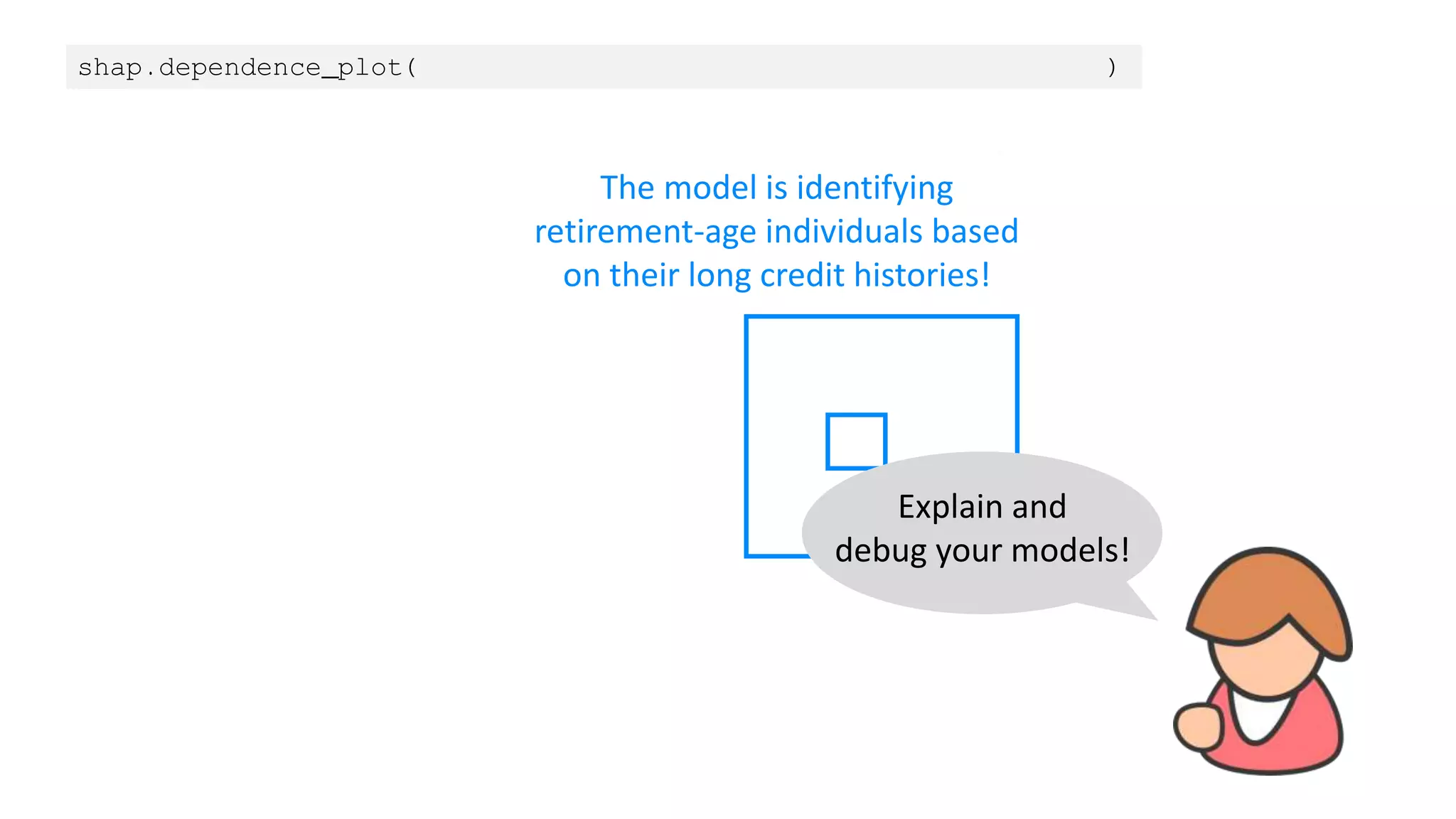
shap.force_plot(ex.expected_value, shap_values[john_ind,:], X.iloc[john_ind,:])
Why does 46 years of credit history increase
the risk of payment problems?](https://image.slidesharecdn.com/1140amgpscottlundbergfinalv2-191022184911/75/Scott-Lundberg-Microsoft-Research-Explainable-Machine-Learning-with-Shapley-Values-H2O-World-NYC-2019-13-2048.jpg)
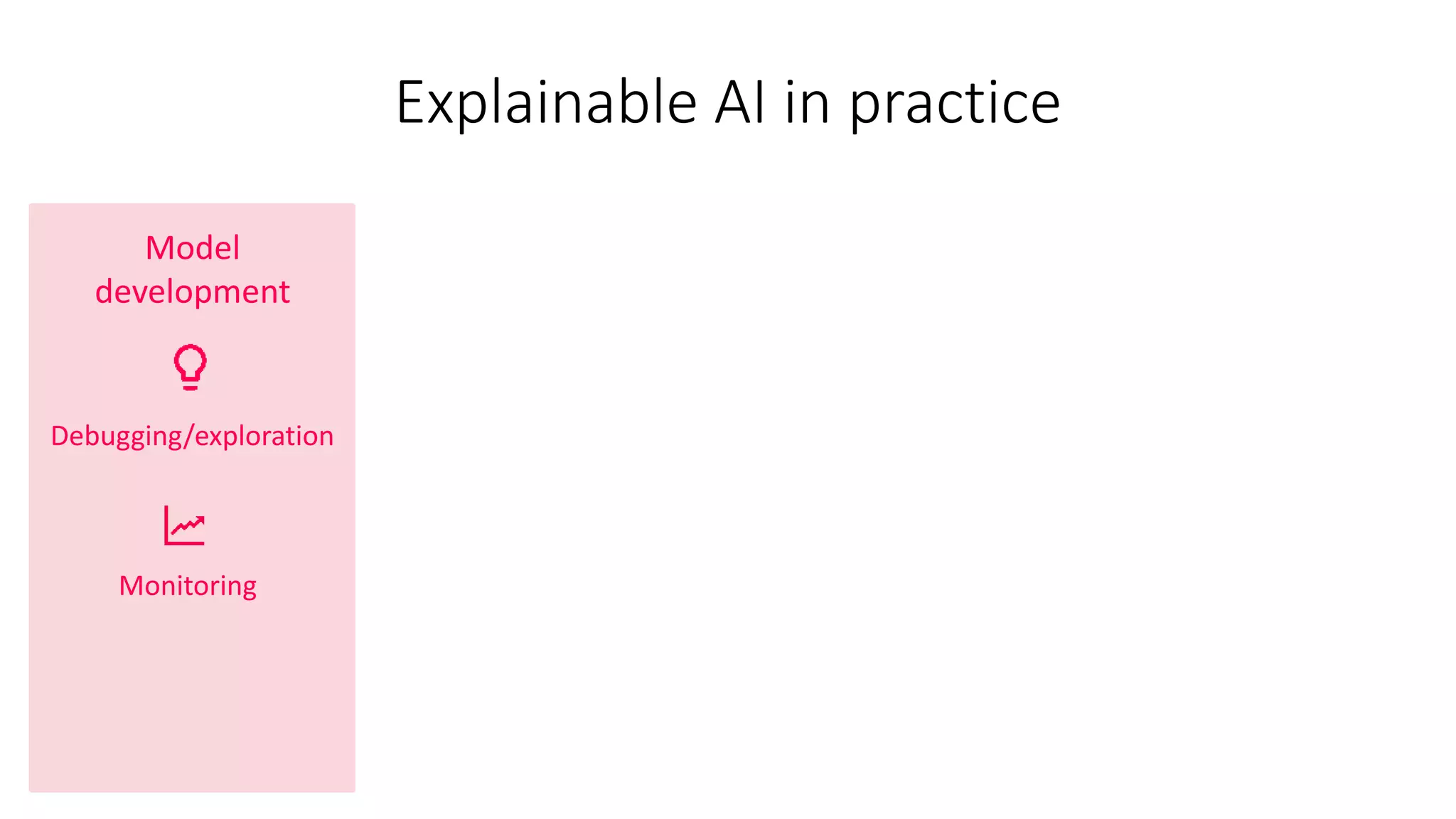

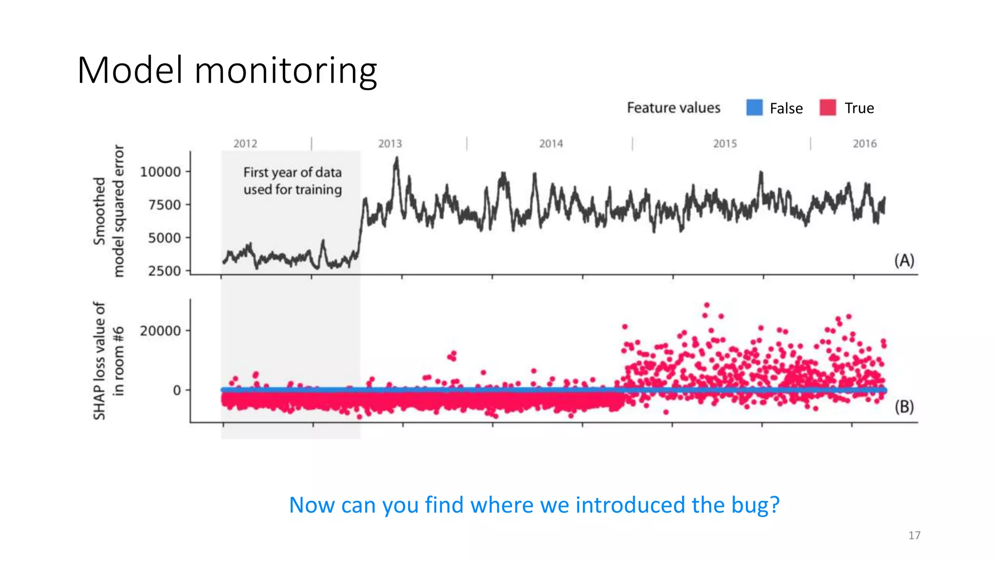

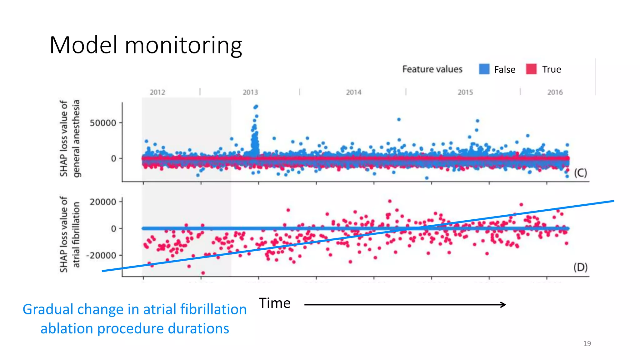
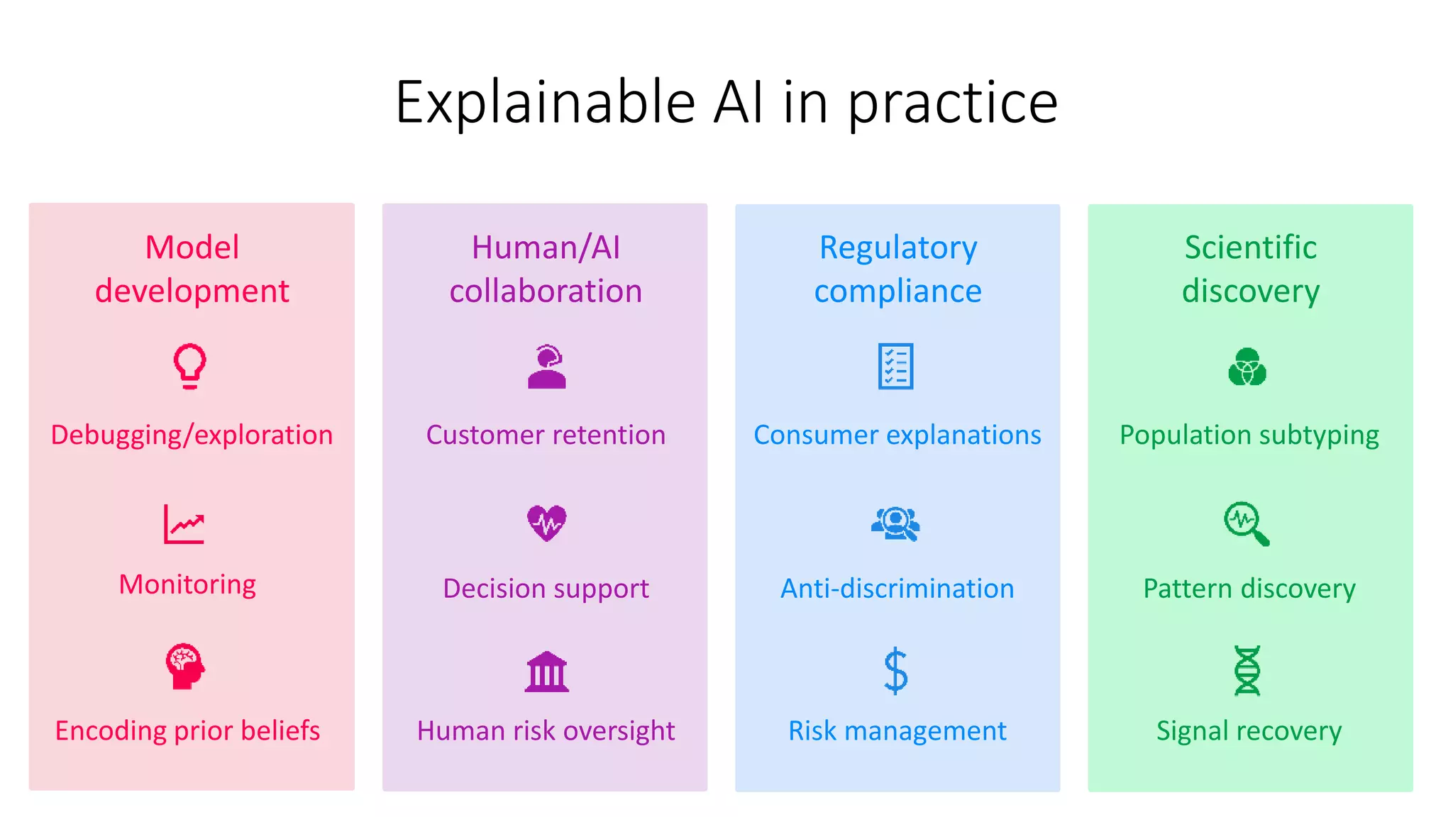


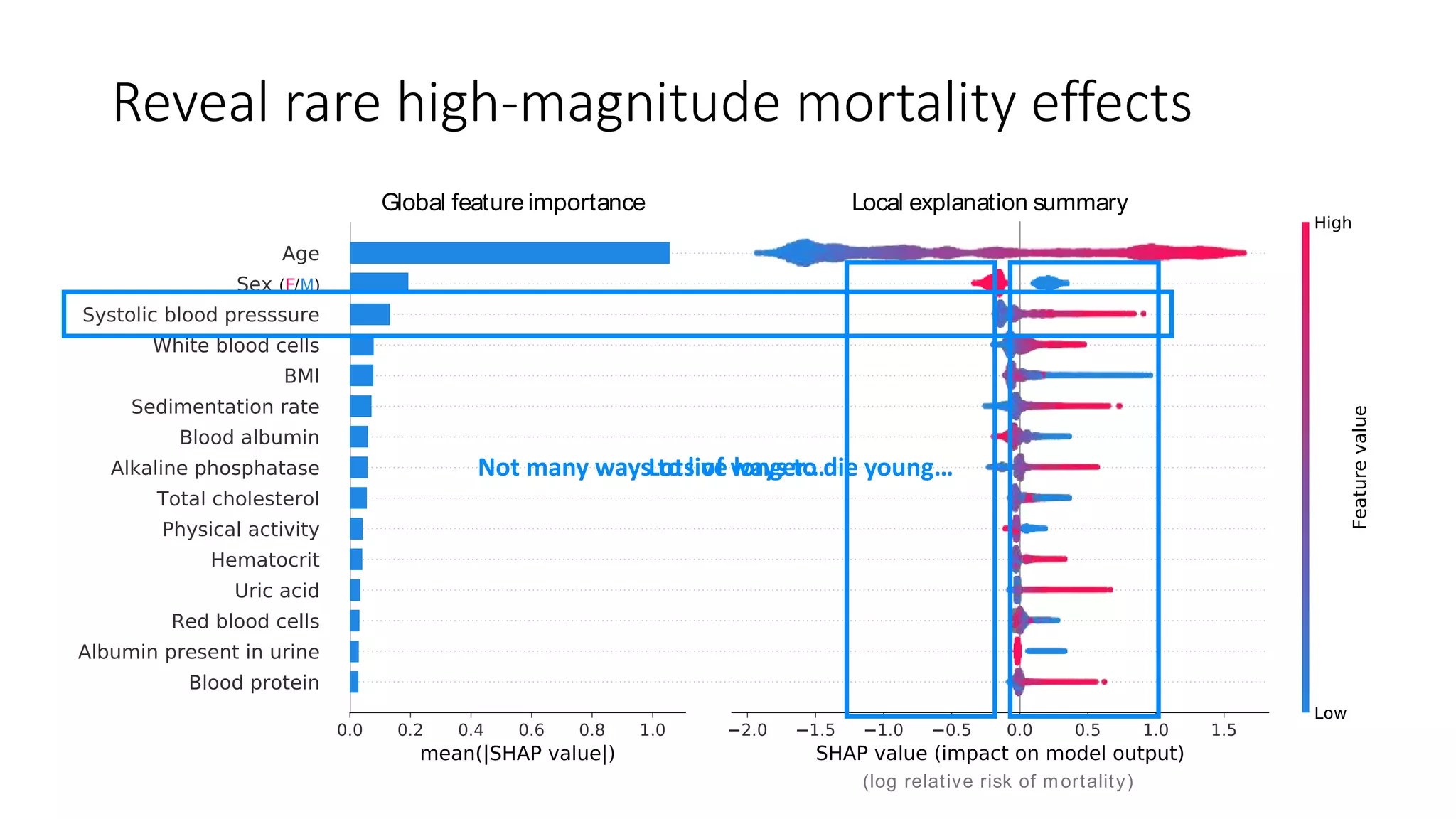

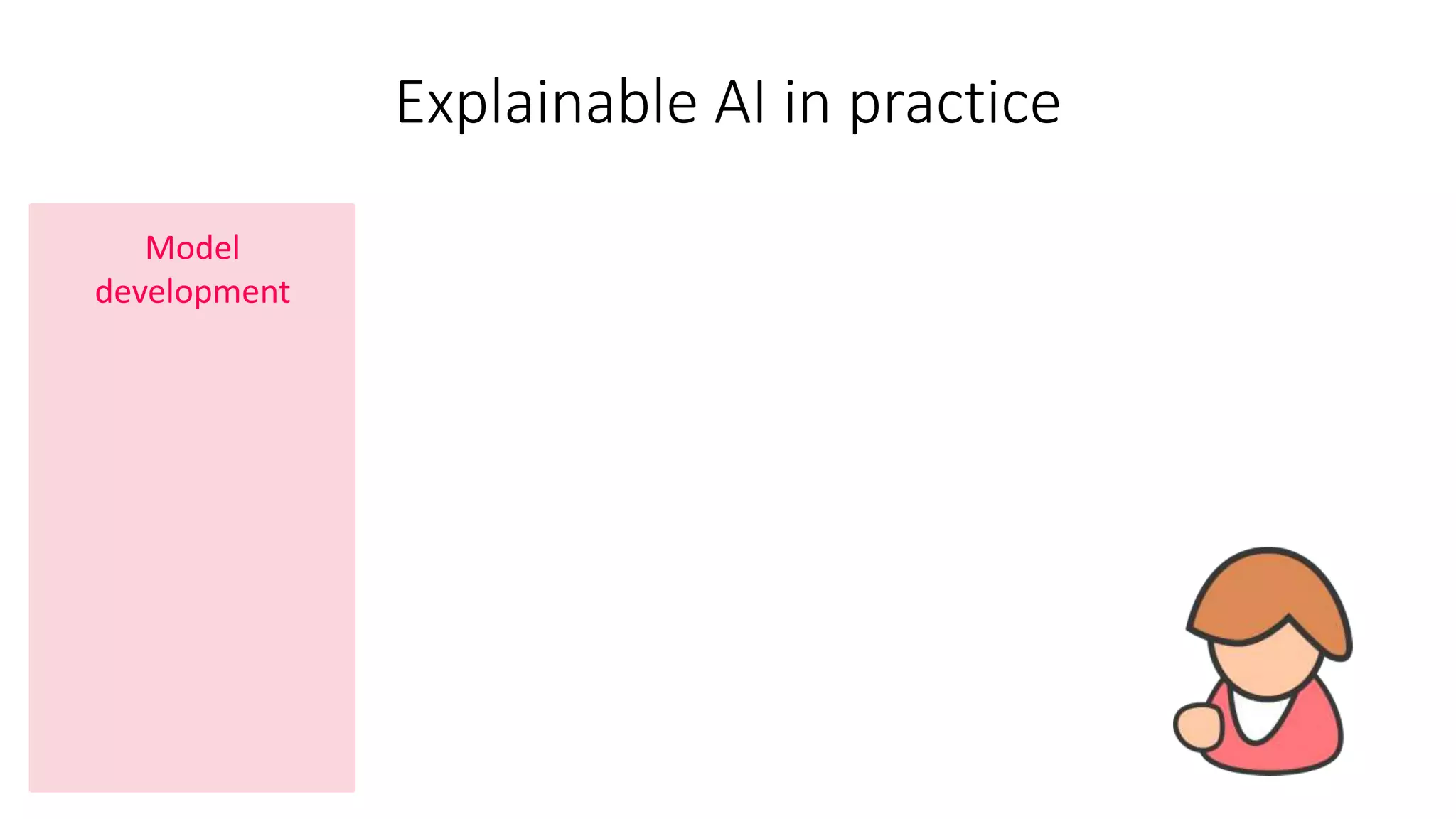
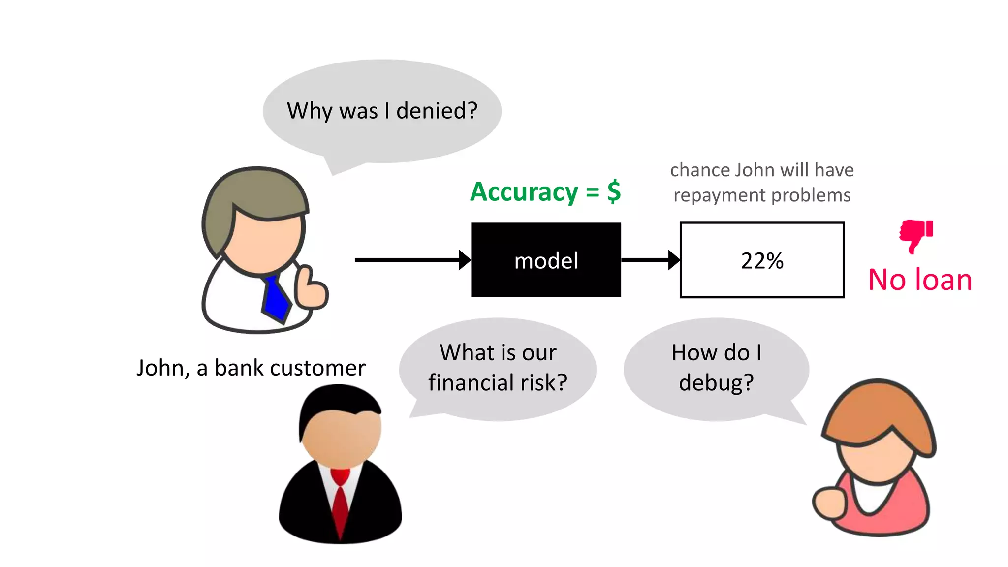
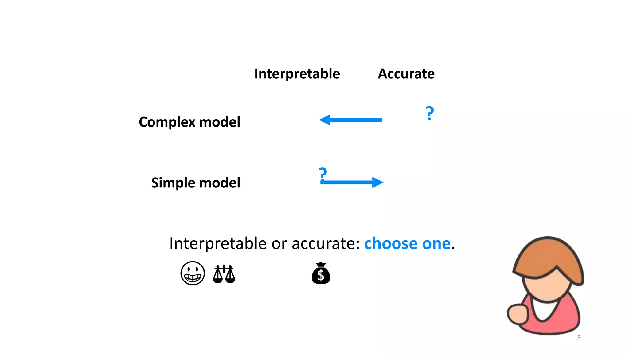
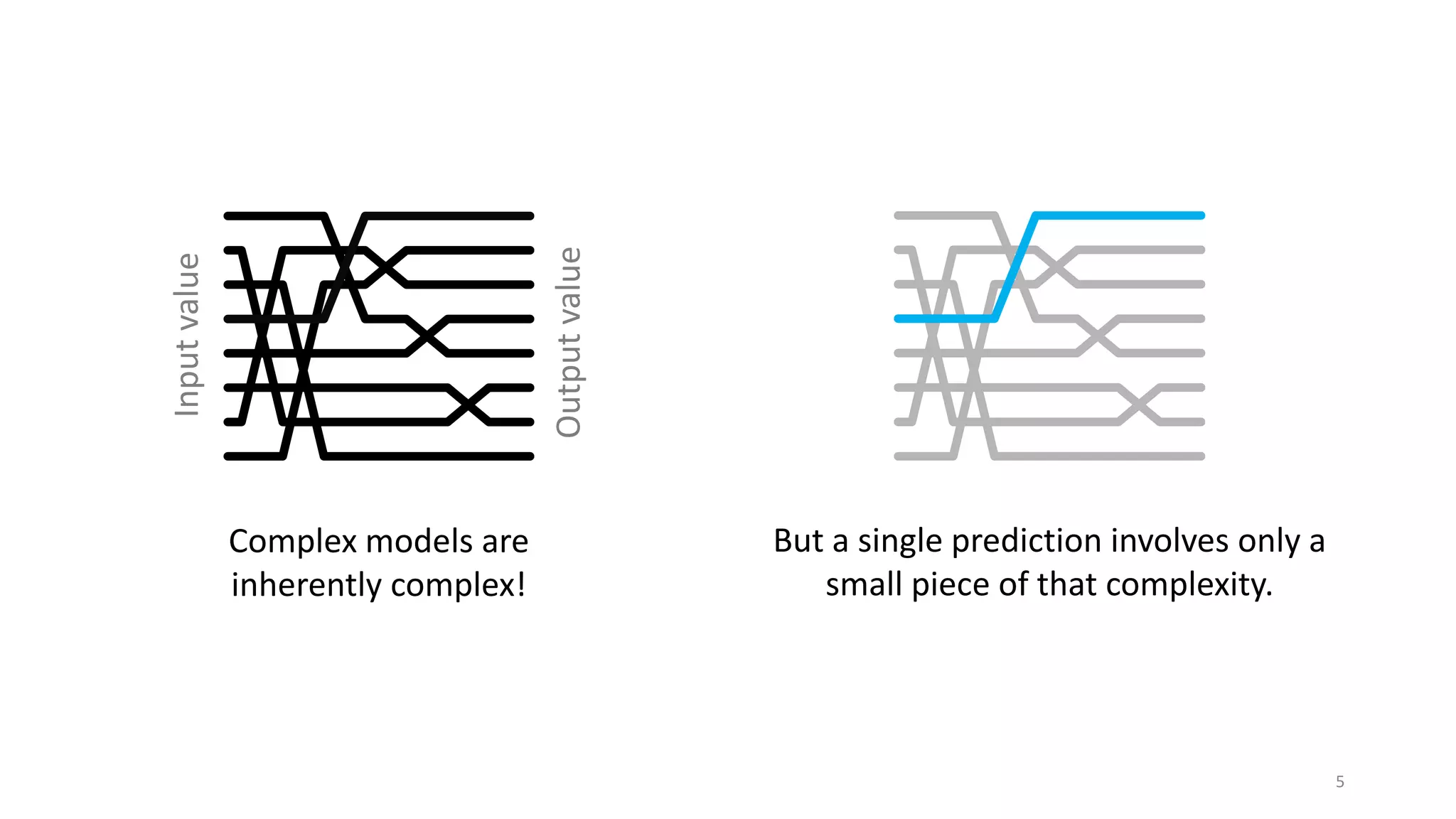
The document discusses the use of Shapley values in explainable machine learning, highlighting their importance for understanding and debugging complex models in financial risk assessment and healthcare. It emphasizes the balance between model accuracy and interpretability, the significance of feature attributions, and properties such as additivity and monotonicity. The examples illustrate how Shapley values can help explain predictions and identify potential issues in model performance, ensuring accountability and transparency in AI applications.


![[DSC Europe 24] Orsalia Andreou - Fostering Trust in AI-Driven Finance](https://cdn.slidesharecdn.com/ss_thumbnails/orsaliaandreoufosteringtrustinai-drivenfinance-250216113615-6aa23936-thumbnail.jpg?width=640&height=640&fit=bounds)


