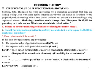
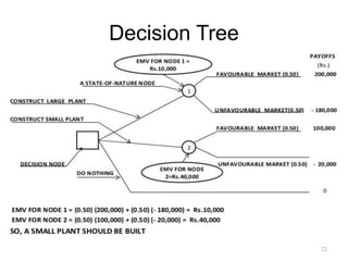
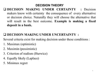
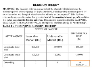
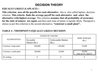
UNIT – V : DECISION THEORY
Syllabus: Decision theory: Risk and uncertainty in decision-making
– minimax, maximin and regret criterion – Hurwicz and Laplace
criteria in decision making – decision tree analysis.
1
What is Decision-making?
• Decision making is an integral part of
management planning, organizing, controlling
processes.
• The decision maker selects one strategy
(course of action) over others depending on
some criteria, like utility, sales, cost or rate of
return.
2
Types of Decisions
• Strategic Decision – Concerned with external
environment of the organization.
• Administrative Decision – Concerned with
structuring and acquisition of the
organization’s resources so as to optimize the
performance of the organization.
• Operating Decision – Concerned with day to
day operations of the organization such as
pricing, production scheduling, inventory
levels, etc.
3
Terminologies
• Course of action: refers to the decision
alternatives or actions that is been chosen by the
decision-maker.
• States of nature: Exhaustive list of possible
future events/alternatives. Decision maker has
no direct control over the occurrence of
particular event.
• Payoff: Effectiveness associated with specified
combination of a course of action and state of
nature. Also known as profits or conditional
values.
4
• TYPES OF DECISION MAKING ENVIRONMENTS
 DECISION MAKING UNDER CERTAINTY
 DECISION MAKING UNDER UNCERTAINTY
 DECISION MAKING UNDER RISK
SIX STEPS IN DECISION MAKING :
 Clearly define the problem in hand
 List the possible alternatives
 Identify the possible outcomes or states of nature
 List the payoff or profit of each combination of alternatives &
outcomes
 Select one of the mathematical decision theory models
 Apply the model and make your decision
5
DECISION THEORY
 DECISION MAKING UNDER CERTAINTY : Decision
makers know with certainty the consequence of every alternative
or decision choice. Naturally they will choose the alternative that
will result in the best outcome. Example is making a fixed
deposit in a bank.
 DECISION MAKING UNDER UNCERTAINTY :
Several criteria exist for making decision under these conditions :
1. Maximax (optimistic)
2. Maximin (pessimistic)
3. Criterion of realism (Hurwicz)
4. Equally likely (Laplace)
5. Minimax regret
6
DECISION THEORY
A CASE STUDY
• John Thompson is the President of Stewarts & Lloyds of India ltd.
• John Thompson’s problem is to identify whether to expand his
product line by manufacturing and marketing a new product :
washing machine.
• In order to make a proposal for submitting to his board of directors,
Thompson thought of following three alternatives that are available
to him.
1. To construct a large new plant to manufacture the washing
machine
2. To construct a small plant to manufacture the washing machine
3. No plant at all ( that is he has the option of not developing the
new product line).
7
DECISION THEORY
• Thompson determines that there are only two possible state of
natures :
1. The market for the washing machine could be favorable,
meaning that there is a high demand for the product
2. it could be unfavorable, meaning that there is a low demand
for the washing machine.
John Thompson evaluated the profits associated with various
outcomes. He thinks :
 With a favorable market, a large facility would result in a
profit of Rs.2,00,000 to his firm. But Rs.2,00,000 is a
conditional value because Thompson's receiving the money is
conditional upon both his building a large factory and
having a good market.
 The large facility and unfavorable market would result in net
loss of Rs.1,80,000. 8
DECISION THEORY
 A small plant with a favorable market would result in a net
profit of Rs.100,000 .
 A small plant with unfavorable market would result in a net
loss of Rs.20,000 .
 doing nothing, that is neither to make large facility nor a small
plant, in either market would result in no profits.
The decision table or payoff table for Thompson's conditional
values is shown in table on next slide .
9
DECISION THEORY
ALTERNATIVES STATES OF NATURE
Favorable
Market (Rs.)
Unfavorable
Market (Rs.)
Construct a
Large plant
200,000 - 180,000
Construct a
Small plant
100,000 - 20,000
Do nothing 0 0
10
DECISION THEORY
MAXIMAX : The maximax criterion is used to find the alternative that maximises the
maximum payoff. First locate the maximum payoff for each alternative, and then pick that
alternative with the maximum number. It locates the alternative with the highest possible gain :
therefore it is called an optimistic decision criteria. Thompson’s maximax choice is the first
alternative “construct a large plant”.
TABLE 1 : THOMPSON’S MAXIMAX DECISION
ALTERNATIVES STATES OF NATURE MAXIMUM IN A
ROW (Rs.)
Favorable
Market (Rs.)
Unfavorable
Market (Rs.)
Construct a large
plant
200,000 -180,000 200,000
MAXIMAX
Construct a small
plant
100,000 -20,000 100,000
Do nothing 0 0 0
11
DECISION THEORY
MAXIMIN : The maximin criterion is used to find the alternative that maximises the
minimum payoff or consequence for every alternative. First locate the minimum payoff for
each alternative and then pick that alternative with the maximum payoff. This decision
criterion locates the alternative that gives the best of the worst (minimum) payoffs, and thus
it is called a pessimistic decision criterion. This criterion guarantees that the payoff WILL
BE AT LEAST THE MAXIMIN VALUE. Thompson’s maximin choice is “do nothing”.
TABLE 2 : THOMPSON’S MAXIMIN DECISION
ALTERNATIVES
STATES OF NATURE
MINIMUM IN A
ROW
(Rs.)
Favorable
Market (Rs.)
Unfavorable
Market (Rs.)
Construct a large
plant
200,000 - 180,000 - 180,000
Construct a small
plant
100,000 - 20,000 - 20,000
Do nothing 0 0 0
MAXIMIN
12
DECISION THEORY
CRITERON OF REALISM (HURWICZ CRITERION)
The criterion of realism is a compromise between an optimistic and a pessimistic decision. A
coefficient of realism (α ) is used to measure the degree of optimism of the decision
maker. this coefficient, α lies between o and 1. The weighted average is computed as follows:
Weighted average = (α) x (maximum in row) + (1 – α) x (minimum in row)
In the given case, John Thompson sets α = 0.80 and thus the best decision would be to
construct a large plant as shown in table 3 below.
TABLE 3 : THOMPSON’S CRITERION OF REALISM DECISION
ALTERNATIVES
STATES OF NATURE CRITERON OF REALISM
OR WEIGHTED
AVERAGE
(α = 0.80)
Favorable
Market (Rs.)
Unfavorable Market
(Rs.)
Construct a large plant 200,000 - 180,000
Construct a small plant 100,000 -20,000 76,000
Do nothing 0 0 0
Rs. 1,24,000
REALISM
13
DECISION THEORY
EQUALLY LIKELY (LAPLACE) :
This criterion uses all the payoffs for each alternative . this is also called laplace, decision
criterion. This criteria finds the average payoff for each alternative and select the
alternative with highest average. This criterion assumes that all probability of occurance
for the state of natures are equal, and thus each state of nature is equally likely. Thompson’s
choice as per this criterion is the second alternative, “construct a small plant”.
TABLE 4 : THOMPSON’S EQUALLY LIKELY DECISION
ALTERNATIVES
STATES OF NATURE
ROW AVERAGE
(Rs.)
Favorable
Market (Rs.)
Unfavorable Market
(Rs.)
Construct a large plant 200,000 - 180,000 10,000
Construct a small plant 100,000 - 20,000
Do nothing 0 0 0
40,000
EQUALLY LIKELY
14
DECISION THEORY
MINIMAX REGRET
This decision criterion is based on opportunity loss or regret. The opportunity loss or regret is the
amount lost by not picking the best alternative in a given state of nature. The first step is to create the
opportunity loss table. Opportunity loss for any state of nature , or any column, is calculated by
subtracting each payoff in the column from the best payoff in the same column.
Thompson’s opportunity loss table is shown in table 5. Using the opportunity loss table, the minimax
regret criterion finds the alternative that minimises the maximum opportunity loss within each
alternative.First find the maximum opportunity loss for each alternative. Next, looking at these maximum
values, pick that alternative with minimum number. We can see that minimax regret choice is the second
alternative, “construct a small plant”.
TABLE 5 : OPPORTUNITY LOSS TABLE
ALTERNATIVES
STATES OF NATURE
Favorable
Market (Rs.)
Unfavorable Market
(Rs.)
MAXIMUM IN A ROW
Construct a large plant 0
[200,000 – 200,000]
180,000
[0 - ( - 180,000)]
180,000
Construct a small plant 100,000
[200,000 – 100,000]
20,000
[0 - ( - 20,000)]
100,000
MINIMAX
Do nothing 200,000
[200,000 - 0]
0
[0 - 0]
200,000 15
DECISION THEORY
 DECISION MAKING UNDER RISK
Decision making under risk is a decision situation in which several possible state of nature
may occur and the probabilities of these states of nature are known. The decision under
risk are taken based on following :
 Expected monetary value or expected value (EMV)
 Expected value of perfect information (EVPI)
 Expected opportunity loss (EOL)
EXPECTED MONETARY VALUE
The expected monetary value (EMV) for an alternative is just the sum of products of
payoffs and probability of each state of nature.
EMV (Alternative ,i) = (Payoff of first state of nature) x ( Probability of first state of
nature)
+ (Payoff of second state of nature) x (Probability of second state of
nature)
+ (Payoff of third state of nature) x (Probability of third state of nature)
+ …………..+ (Pay of last state of nature) x (Probability of last state of nature)
The alternative with maximum EMV is then chosen.
Suppose Thompson now believes that the probability of a favorable market is exactly the
same as the probability of an unfavorable market.
16
DECISION THEORY
SOLUTION BY USING EMV METHOD :
EMV (Large Plant) = (0.50) x (Rs.200,000) + (0.50) x (-Rs.180,000) = Rs.10,000
EMV ( Small Plant) = (0.50) x (Rs.100,000) + (0.50) x (-Rs.20,000) = Rs.40,000
EMV (Do Nothing) = (0.50) x (Rs.0) + (0.50) x (Rs.0) = Rs.0
THE LARGEST EXPECTED VALUE OF Rs.40,000 results from the second alternative
“construct a small plant”. Thus Thompson would proceed to set up small plant.
TABLE 6 : Decision Table with Probabilities and EMVs for John Thompson
17
Alternatives States of Nature EMV
Favorable
Market
Unfavorable
Market
Construct Large
Plant
200,000 - 180,000 10,000
Construct Small
Plant
100,000 - 20,000 40,000
Maximum Value
Do Nothing 0 0 0
Probability 0.50 0.50
DECISION THEORY
 EXPECTED VALUE OF PERFECT INFORMATION (EVPI)
Suppose, John Thompson has been approached by a marketing consultant that they are
willing to help John with some perfect information whether the market is favorable for the
proposed product enabling John to take correct decision and prevent him from making a very
expensive mistake. Marketing consultant would charge John Thompson Rs.65,000 for
providing such information. What John should do in this situation ?
1. Should he hire the marketing consultant for making the market study ?
2. Even if the information provided is perfectly accurate, is it worth to pay Rs.65,000 to
marketing consultant?
3.If not, what would it be worth ?
In this case, two related terms are investigated :
1. The expected value of perfect information (EVPI), and
2. The expected value with perfect information (EVwPI)
EVwPI = (Best payoff for first state of nature) x (Probability of first state of nature) +
(Best payoff for second state of nature) x (Probability for second state of
nature)
+ ……………+ (Best payoff for last state of nature) x (Probability for last state of
nature)
EVPI = EVwPI - Maximum EMV
18
DECISION THEORY
EVPI With respect to table 6 is calculated as follows :
1. The best payoff for the state of nature “favorable market” is Rs.200,000. The best
payoff for the state of nature “unfavorable market” is Rs.0.
Now, EVwPI = (Rs.200,000) (0.50) + (Rs.0) (0.50) = Rs.100,000
Thus, if John had perfect information, the payoff would average Rs.100,000
2.The maximum EMV without additional information is Rs.40,000(from table 6)
So, EVPI = (Expected value with perfect information) – (Maximum EMV)
= Rs.100,000 - Rs.40,000 = Rs.60,000
Thus, at best John Thompson would be willing to pay for perfect information is
Rs.60,000 based on assumption that the probability of each state of nature is 0.50.
 EXPECTED OPPORTUNITY LOSS
An alternative approach is to maximise EMV by minimising expected opportunity
loss. First an opportunity loss table is constructed. Then the EOL is computed for each
alternative by multiplying the opportunity loss by the probability and adding these
together.
19
DECISION THEORY
Using table 5, we compute the EOL for each alternative as follows :
EOL(Construct Large plant) = (0.50) (Rs.0) + (0.50) (Rs.180,000) = Rs.90,000
EOL (Construct a small plant) = (0.50) (Rs.100,000) + (0.50) (Rs.20,000) = Rs.60,000
EOL (Do nothing) = (0.50) (Rs.200,000) + (0.50) (Rs.0) = Rs.100,000
From the EOL Table 7 , we see that the best decision would be the second alternative :
“construct a small plant”.
TABLE 7 : EOL TABLE FOR JOHN THOMPSON
ALTERNATIVES
STATES OF NATURE
EOL
Favorable
Market (Rs.)
Unfavorable Market
(Rs.)
Construct a large plant 0 180,000 90,000
Construct a small plant 100,000 20,000 60,000
Minimum Value
Do nothing 200,000 0 100,000
Probabilities 0.50 0.50
20
DECISION TREES
Any problem that can be presented in a decision table can also be graphically
illustrated by a decision tree. All decision trees contains decision nodes and
state of nature nodes.
 Decision nodes are represented by squares from which one or several
alternatives may be chosen
 State-of-nature nodes are represented by circles out of which one or more
state-of-nature will occur
In drawing the tree, we begin at the left and move to the right. Branches from
the squares (decision nodes) represent alternatives, and branches from the
circles (state-of-nature node) represent the state of nature.
Figure 1 gives the basic decision tree of John Thompson problem.
Five steps of decision tree analysis :
1. Define the problem
2. Draw the decision tree
3. Assign probabilities to the state of nature
4. Estimate payoffs for each possible combination of alternative and state of nature
5. SOLVE THE PROBLEM BY COMPUTING EXPECTED MONETARY VALUES
(EMVs) FOR EACH STATE OF NATURE NODE. This is done by starting at the right
of the tree and working back to decision node on the left. At each decision node, the
alternative with best EMV is selected.
21
Decision Tree
22

Decision Theory Notes operations research.pdf

  • 1.
    UNIT – V: DECISION THEORY Syllabus: Decision theory: Risk and uncertainty in decision-making – minimax, maximin and regret criterion – Hurwicz and Laplace criteria in decision making – decision tree analysis. 1
  • 2.
    What is Decision-making? •Decision making is an integral part of management planning, organizing, controlling processes. • The decision maker selects one strategy (course of action) over others depending on some criteria, like utility, sales, cost or rate of return. 2
  • 3.
    Types of Decisions •Strategic Decision – Concerned with external environment of the organization. • Administrative Decision – Concerned with structuring and acquisition of the organization’s resources so as to optimize the performance of the organization. • Operating Decision – Concerned with day to day operations of the organization such as pricing, production scheduling, inventory levels, etc. 3
  • 4.
    Terminologies • Course ofaction: refers to the decision alternatives or actions that is been chosen by the decision-maker. • States of nature: Exhaustive list of possible future events/alternatives. Decision maker has no direct control over the occurrence of particular event. • Payoff: Effectiveness associated with specified combination of a course of action and state of nature. Also known as profits or conditional values. 4
  • 5.
    • TYPES OFDECISION MAKING ENVIRONMENTS  DECISION MAKING UNDER CERTAINTY  DECISION MAKING UNDER UNCERTAINTY  DECISION MAKING UNDER RISK SIX STEPS IN DECISION MAKING :  Clearly define the problem in hand  List the possible alternatives  Identify the possible outcomes or states of nature  List the payoff or profit of each combination of alternatives & outcomes  Select one of the mathematical decision theory models  Apply the model and make your decision 5
  • 6.
    DECISION THEORY  DECISIONMAKING UNDER CERTAINTY : Decision makers know with certainty the consequence of every alternative or decision choice. Naturally they will choose the alternative that will result in the best outcome. Example is making a fixed deposit in a bank.  DECISION MAKING UNDER UNCERTAINTY : Several criteria exist for making decision under these conditions : 1. Maximax (optimistic) 2. Maximin (pessimistic) 3. Criterion of realism (Hurwicz) 4. Equally likely (Laplace) 5. Minimax regret 6
  • 7.
    DECISION THEORY A CASESTUDY • John Thompson is the President of Stewarts & Lloyds of India ltd. • John Thompson’s problem is to identify whether to expand his product line by manufacturing and marketing a new product : washing machine. • In order to make a proposal for submitting to his board of directors, Thompson thought of following three alternatives that are available to him. 1. To construct a large new plant to manufacture the washing machine 2. To construct a small plant to manufacture the washing machine 3. No plant at all ( that is he has the option of not developing the new product line). 7
  • 8.
    DECISION THEORY • Thompsondetermines that there are only two possible state of natures : 1. The market for the washing machine could be favorable, meaning that there is a high demand for the product 2. it could be unfavorable, meaning that there is a low demand for the washing machine. John Thompson evaluated the profits associated with various outcomes. He thinks :  With a favorable market, a large facility would result in a profit of Rs.2,00,000 to his firm. But Rs.2,00,000 is a conditional value because Thompson's receiving the money is conditional upon both his building a large factory and having a good market.  The large facility and unfavorable market would result in net loss of Rs.1,80,000. 8
  • 9.
    DECISION THEORY  Asmall plant with a favorable market would result in a net profit of Rs.100,000 .  A small plant with unfavorable market would result in a net loss of Rs.20,000 .  doing nothing, that is neither to make large facility nor a small plant, in either market would result in no profits. The decision table or payoff table for Thompson's conditional values is shown in table on next slide . 9
  • 10.
    DECISION THEORY ALTERNATIVES STATESOF NATURE Favorable Market (Rs.) Unfavorable Market (Rs.) Construct a Large plant 200,000 - 180,000 Construct a Small plant 100,000 - 20,000 Do nothing 0 0 10
  • 11.
    DECISION THEORY MAXIMAX :The maximax criterion is used to find the alternative that maximises the maximum payoff. First locate the maximum payoff for each alternative, and then pick that alternative with the maximum number. It locates the alternative with the highest possible gain : therefore it is called an optimistic decision criteria. Thompson’s maximax choice is the first alternative “construct a large plant”. TABLE 1 : THOMPSON’S MAXIMAX DECISION ALTERNATIVES STATES OF NATURE MAXIMUM IN A ROW (Rs.) Favorable Market (Rs.) Unfavorable Market (Rs.) Construct a large plant 200,000 -180,000 200,000 MAXIMAX Construct a small plant 100,000 -20,000 100,000 Do nothing 0 0 0 11
  • 12.
    DECISION THEORY MAXIMIN :The maximin criterion is used to find the alternative that maximises the minimum payoff or consequence for every alternative. First locate the minimum payoff for each alternative and then pick that alternative with the maximum payoff. This decision criterion locates the alternative that gives the best of the worst (minimum) payoffs, and thus it is called a pessimistic decision criterion. This criterion guarantees that the payoff WILL BE AT LEAST THE MAXIMIN VALUE. Thompson’s maximin choice is “do nothing”. TABLE 2 : THOMPSON’S MAXIMIN DECISION ALTERNATIVES STATES OF NATURE MINIMUM IN A ROW (Rs.) Favorable Market (Rs.) Unfavorable Market (Rs.) Construct a large plant 200,000 - 180,000 - 180,000 Construct a small plant 100,000 - 20,000 - 20,000 Do nothing 0 0 0 MAXIMIN 12
  • 13.
    DECISION THEORY CRITERON OFREALISM (HURWICZ CRITERION) The criterion of realism is a compromise between an optimistic and a pessimistic decision. A coefficient of realism (α ) is used to measure the degree of optimism of the decision maker. this coefficient, α lies between o and 1. The weighted average is computed as follows: Weighted average = (α) x (maximum in row) + (1 – α) x (minimum in row) In the given case, John Thompson sets α = 0.80 and thus the best decision would be to construct a large plant as shown in table 3 below. TABLE 3 : THOMPSON’S CRITERION OF REALISM DECISION ALTERNATIVES STATES OF NATURE CRITERON OF REALISM OR WEIGHTED AVERAGE (α = 0.80) Favorable Market (Rs.) Unfavorable Market (Rs.) Construct a large plant 200,000 - 180,000 Construct a small plant 100,000 -20,000 76,000 Do nothing 0 0 0 Rs. 1,24,000 REALISM 13
  • 14.
    DECISION THEORY EQUALLY LIKELY(LAPLACE) : This criterion uses all the payoffs for each alternative . this is also called laplace, decision criterion. This criteria finds the average payoff for each alternative and select the alternative with highest average. This criterion assumes that all probability of occurance for the state of natures are equal, and thus each state of nature is equally likely. Thompson’s choice as per this criterion is the second alternative, “construct a small plant”. TABLE 4 : THOMPSON’S EQUALLY LIKELY DECISION ALTERNATIVES STATES OF NATURE ROW AVERAGE (Rs.) Favorable Market (Rs.) Unfavorable Market (Rs.) Construct a large plant 200,000 - 180,000 10,000 Construct a small plant 100,000 - 20,000 Do nothing 0 0 0 40,000 EQUALLY LIKELY 14
  • 15.
    DECISION THEORY MINIMAX REGRET Thisdecision criterion is based on opportunity loss or regret. The opportunity loss or regret is the amount lost by not picking the best alternative in a given state of nature. The first step is to create the opportunity loss table. Opportunity loss for any state of nature , or any column, is calculated by subtracting each payoff in the column from the best payoff in the same column. Thompson’s opportunity loss table is shown in table 5. Using the opportunity loss table, the minimax regret criterion finds the alternative that minimises the maximum opportunity loss within each alternative.First find the maximum opportunity loss for each alternative. Next, looking at these maximum values, pick that alternative with minimum number. We can see that minimax regret choice is the second alternative, “construct a small plant”. TABLE 5 : OPPORTUNITY LOSS TABLE ALTERNATIVES STATES OF NATURE Favorable Market (Rs.) Unfavorable Market (Rs.) MAXIMUM IN A ROW Construct a large plant 0 [200,000 – 200,000] 180,000 [0 - ( - 180,000)] 180,000 Construct a small plant 100,000 [200,000 – 100,000] 20,000 [0 - ( - 20,000)] 100,000 MINIMAX Do nothing 200,000 [200,000 - 0] 0 [0 - 0] 200,000 15
  • 16.
    DECISION THEORY  DECISIONMAKING UNDER RISK Decision making under risk is a decision situation in which several possible state of nature may occur and the probabilities of these states of nature are known. The decision under risk are taken based on following :  Expected monetary value or expected value (EMV)  Expected value of perfect information (EVPI)  Expected opportunity loss (EOL) EXPECTED MONETARY VALUE The expected monetary value (EMV) for an alternative is just the sum of products of payoffs and probability of each state of nature. EMV (Alternative ,i) = (Payoff of first state of nature) x ( Probability of first state of nature) + (Payoff of second state of nature) x (Probability of second state of nature) + (Payoff of third state of nature) x (Probability of third state of nature) + …………..+ (Pay of last state of nature) x (Probability of last state of nature) The alternative with maximum EMV is then chosen. Suppose Thompson now believes that the probability of a favorable market is exactly the same as the probability of an unfavorable market. 16
  • 17.
    DECISION THEORY SOLUTION BYUSING EMV METHOD : EMV (Large Plant) = (0.50) x (Rs.200,000) + (0.50) x (-Rs.180,000) = Rs.10,000 EMV ( Small Plant) = (0.50) x (Rs.100,000) + (0.50) x (-Rs.20,000) = Rs.40,000 EMV (Do Nothing) = (0.50) x (Rs.0) + (0.50) x (Rs.0) = Rs.0 THE LARGEST EXPECTED VALUE OF Rs.40,000 results from the second alternative “construct a small plant”. Thus Thompson would proceed to set up small plant. TABLE 6 : Decision Table with Probabilities and EMVs for John Thompson 17 Alternatives States of Nature EMV Favorable Market Unfavorable Market Construct Large Plant 200,000 - 180,000 10,000 Construct Small Plant 100,000 - 20,000 40,000 Maximum Value Do Nothing 0 0 0 Probability 0.50 0.50
  • 18.
    DECISION THEORY  EXPECTEDVALUE OF PERFECT INFORMATION (EVPI) Suppose, John Thompson has been approached by a marketing consultant that they are willing to help John with some perfect information whether the market is favorable for the proposed product enabling John to take correct decision and prevent him from making a very expensive mistake. Marketing consultant would charge John Thompson Rs.65,000 for providing such information. What John should do in this situation ? 1. Should he hire the marketing consultant for making the market study ? 2. Even if the information provided is perfectly accurate, is it worth to pay Rs.65,000 to marketing consultant? 3.If not, what would it be worth ? In this case, two related terms are investigated : 1. The expected value of perfect information (EVPI), and 2. The expected value with perfect information (EVwPI) EVwPI = (Best payoff for first state of nature) x (Probability of first state of nature) + (Best payoff for second state of nature) x (Probability for second state of nature) + ……………+ (Best payoff for last state of nature) x (Probability for last state of nature) EVPI = EVwPI - Maximum EMV 18
  • 19.
    DECISION THEORY EVPI Withrespect to table 6 is calculated as follows : 1. The best payoff for the state of nature “favorable market” is Rs.200,000. The best payoff for the state of nature “unfavorable market” is Rs.0. Now, EVwPI = (Rs.200,000) (0.50) + (Rs.0) (0.50) = Rs.100,000 Thus, if John had perfect information, the payoff would average Rs.100,000 2.The maximum EMV without additional information is Rs.40,000(from table 6) So, EVPI = (Expected value with perfect information) – (Maximum EMV) = Rs.100,000 - Rs.40,000 = Rs.60,000 Thus, at best John Thompson would be willing to pay for perfect information is Rs.60,000 based on assumption that the probability of each state of nature is 0.50.  EXPECTED OPPORTUNITY LOSS An alternative approach is to maximise EMV by minimising expected opportunity loss. First an opportunity loss table is constructed. Then the EOL is computed for each alternative by multiplying the opportunity loss by the probability and adding these together. 19
  • 20.
    DECISION THEORY Using table5, we compute the EOL for each alternative as follows : EOL(Construct Large plant) = (0.50) (Rs.0) + (0.50) (Rs.180,000) = Rs.90,000 EOL (Construct a small plant) = (0.50) (Rs.100,000) + (0.50) (Rs.20,000) = Rs.60,000 EOL (Do nothing) = (0.50) (Rs.200,000) + (0.50) (Rs.0) = Rs.100,000 From the EOL Table 7 , we see that the best decision would be the second alternative : “construct a small plant”. TABLE 7 : EOL TABLE FOR JOHN THOMPSON ALTERNATIVES STATES OF NATURE EOL Favorable Market (Rs.) Unfavorable Market (Rs.) Construct a large plant 0 180,000 90,000 Construct a small plant 100,000 20,000 60,000 Minimum Value Do nothing 200,000 0 100,000 Probabilities 0.50 0.50 20
  • 21.
    DECISION TREES Any problemthat can be presented in a decision table can also be graphically illustrated by a decision tree. All decision trees contains decision nodes and state of nature nodes.  Decision nodes are represented by squares from which one or several alternatives may be chosen  State-of-nature nodes are represented by circles out of which one or more state-of-nature will occur In drawing the tree, we begin at the left and move to the right. Branches from the squares (decision nodes) represent alternatives, and branches from the circles (state-of-nature node) represent the state of nature. Figure 1 gives the basic decision tree of John Thompson problem. Five steps of decision tree analysis : 1. Define the problem 2. Draw the decision tree 3. Assign probabilities to the state of nature 4. Estimate payoffs for each possible combination of alternative and state of nature 5. SOLVE THE PROBLEM BY COMPUTING EXPECTED MONETARY VALUES (EMVs) FOR EACH STATE OF NATURE NODE. This is done by starting at the right of the tree and working back to decision node on the left. At each decision node, the alternative with best EMV is selected. 21
  • 22.