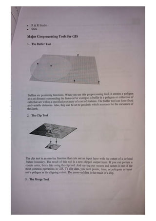
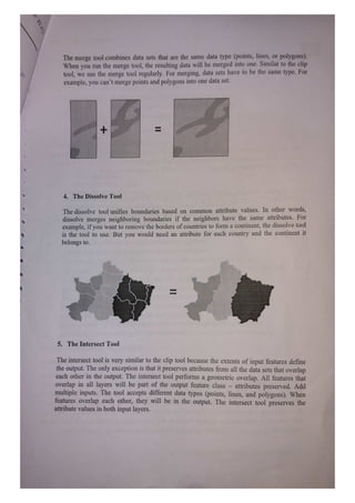
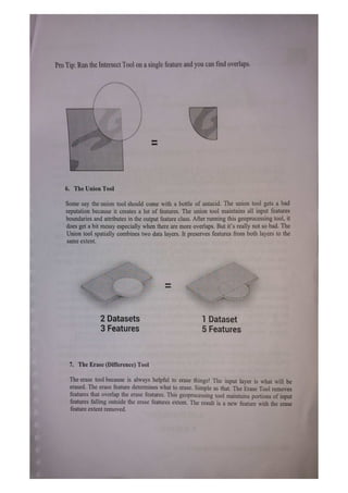
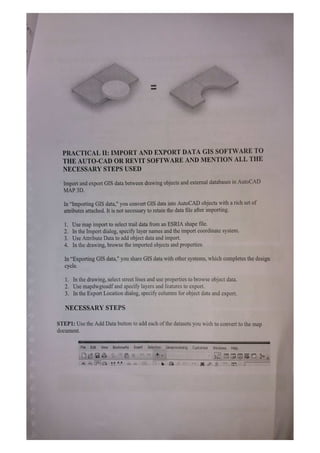
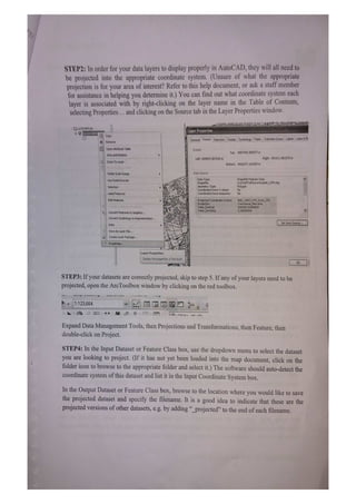
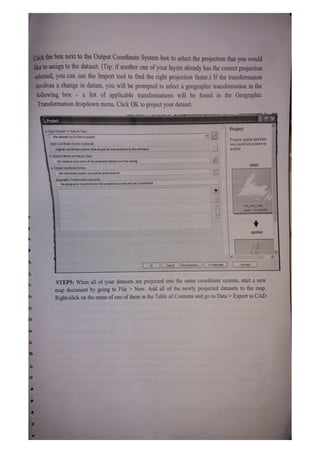
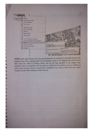
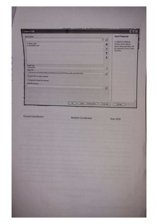
PRACTICAL 1: STUDY OF FUNDAMENTAL TOOLS OF SOFTWARE FOR DATA
PROCESSING
Access GIS software remotely
Virtual Lab (vLab)
The vLab has ArcGIS, GeoDa, and Google Earth Pro. To access vLab on yourpersona
computer, see the instructions provided via the link above.
ArcGIS Online
Use your browser to find, explore, and analyze spatial data. Use the Enterprise login.
When prompted for the URL enter uchicago.
ArcGIS for Desktop
The Research Computing Center provides student copies of ArcGIS for Desktop.
Free desktop GIS software
GeoDa
The premier free and open-source tool for spatial analysis.
QGIS
Free and open-source GIS for creating, editing, visualizing, analyzing, and publishing
spatial data.
Google Earth Pro
Free desktop software for viewing, creating, and displaying spatial data and information.
ggmap for R
For those familiar with R/RStudio, install the ggmap package to visualize and analyze
spatial data.
Web GIS
Popular online tools:
ArcGIS Online
Use your browser to find, explore, and analyze spatial data. Use the Enterprise login. When
prompted for the URL enter uchicago.
Carto
Create maps and apps for business decision making.
Google MyMaps
A fun tool for getting started with web mapping.
OpenStreetMap
The world's leading map made from crowd-sourced, local knowledge. Sign up to start editing
your hometown, or get involved with humanitarian mapping.
Scribble Maps
Like MS Paint for maps. Easy to make a simple map and export as an image
StoryMap JS
From the creators of the popular TimelineJS, present a timeline on a map.
Programming libraries for creating web maps:
D3
A Javascript library following modern web standards. Use to create interactive, data driven webb
maps and charts.
Leaflet
A JavaScript library for creating web maps.
GIS Software in the Market
ArcGIS for Desktop 10.6.1
ArcGIS Pro 2.2.0
ArcGIS Maps for Office (Excel, PowerPoint)
GeoDa
QGIS
Google Earth Pro
Adobe Creative Suite 5 (Illustrator, Photoshop, InDesign)
R&R Studio
Stata
Major Geoprocessing Tools for GIS
1. The Buffer Tool
Buffers are proximity functions. When you use this geoprocessing tool, it creates a polygon
at a set distance surrounding the features.For example, a buffer is a polygon or collection of
cells that are within a specified proximity of a set of features. The buffer tool can have fixed
and variable distances. Also, they can be set to geodesic which accounts for the curvature of
the Earth.
2. The Clip Tool
The clip tool is an overlay function that cuts out an input layer with the extent of a defined
feature boundary. The result ofthis tool is a new clipped output layer. If you can picture a
cookie cutter, this is like using the clip tool. And carving out vectors and rasters is one of the
most common operations in GIS. To clip data, you need points, lines, or polygons as input
and a polygon as the clipping extent. The preserved data is the result of a clip.
3. The Merge Tool
The merge tool combines data sets that are the same data type (points, lines, or polygons).
When you run the merge tool, the resulting data will be merged into one. Similar to the clip
tool, we use the merge tool regularly. For merging, data sets have to be the same type. For
example, you can't merge points and polygons into one data set.
+
4. The Dissolve Tool
The dissolve tool unifies boundaries based on common attribute values. In other words,
dissolve merges neighboring boundaries if the neighbors have the same attributes. For
example, if you want to remove the borders of countries to form a continent, the dissolve tool
is the tool to use. But you would need an attribute for each country and the continent it
belongs to.
5. The Intersect Tool
The interseet tool is very similar to the clip tool because the extents of input features define
the output. The only exception is that it preserves attributes firom all the data sets that overlap
each other in the output. The intersect tool performs a geometric overlap. All features that
overlap in all layers will be part of the output feature class attributes preserved. Add
multiple inputs. The tool accepts different data types (points, lines, and polygons). When
features overlap each other, they will be in the output. The intersect tool preserves the
attribute values in both input layers.
Pro Tip: Run the Intersect Tool on a single feature and you can find overlaps.
6. The Union Tool
Some say the union tool should come with a bottle of antacid. The union tool gets a bad
reputation because it creates a lot of features. The union tool maintains all input features
boundaries and attributes in the output feature class. After running this geoprocessing tool, it
does get a bit messy especially when there are more overlaps. But it's really not so bad. The
Union tool spatially combines two data layers. It preserves features from both layers to the
same extent.
2 Datasets 1
Dataset
3 Features 5 Features
7. The Erase (Difference) Tool
The erase tool because is always helpful to erase things! The input layer is what will be
erased. The erase feature determines what to erase. Simple as that. The Erase Tool removes
features that overlap the erase features. This geoprocessing tool maintains portions of input
features falling outside the erase features extent. The result is a new feature with the erase
feature extent removed.
PRACTICAL II: IMPORT AND EXPORT DATA GIS SOFTWARE TO
THE AUTO-CAD OR REVIT SOFTWARE AND MENTION ALL THE
NECESSARY STEPS USED
Import and export GIS data between drawing objects and external databases in AutoCAD
MAP 3D.
In "Importing GIS data," you convert GIS data into AutoCAD objects with a rich set of
attributes attached. It is not necessary to retain the data file after importing.
1. Use map import to select trail data from an ESRIA shape file.
2. In the Import dialog, specify layer names and the import coordinate system.
3. Use Attribute Data to add object data and import.
4. In the drawing, browse the imported objects and properties.
In "Exporting GIS data," you share GIS data with other systems, which completes the design
cycle.
1. In the drawing, select street lines and use properties to browse object data.
2. Use mapdwgtosdf and specify layers and features to export.
3. In the Export Location dialog, specify columns for object data and export.
NECESSARY STEPS
STEP1: Use the Add Data button to add each ofthe datasets you wish to convert to the map
document.
File Edit View Bookmarks Insert Selection Geoprocessing Customize Windows Help
STEP2: In order for your data layers to display properly in AutoCAD, they will ll nced to
be projected into the appropriate coordinate system. (Unsure of what the appropriate
projection is for your area of interest? Refer to this help document, or ask a staff member
for assistance in helping you determine it.) You can find out what coordinate system each
layer is associated with by right-clicking on the layer name in the Table of Contents,
selecting Properties.. and clicking on the Source tab in the Layer Properties window.
UASTAFE) Layer Properties
COpy
General Souce Selection Disploy Symbology Fields Defrition Query Labels Joins &R
XRemove
Open Atribute Table Extent
Top: 4857445.000077 m
Joins and Relates
Left: 609557.007243 m Righk: 651611.861270 m
Zoom To Layer
Bottom: 4826377, 162654 m
en toPe atle
Visible Scale Range Data Source
ShapefleFeature Class
Data Type:
Shapefile:
Geometry 1ype
Coordinates have Z values:
Coordinates have rneasures: No
Use Symbol Levels
U:STAFFUHitoronkodab6_UTM.shp
Polygon
No
Selection
Label Features
Edt Features Proeccedco0rdinare >ystem:
63 0ne1/
False Easting
alse Northing:
500000.00000000
,00000000
ConvertFeakures to Graphics..
Convert symbology to Representation
Set DetaSource
Data
Save As Layer File..
reate LayerPackage.
rOperues.
Layer Properties
DISplay the properties of this layer
STEP3: If your datasets are correctly projected, skip to step 5. If any of your layers need to be
projected, open the ArcToolbox window by clicking on the red toolbox.
---*****
**
1.:123.664
Expand Data Management Tools, then Projections and Transformations, then Feature, then
double-click on Project.
STEP4: In the Input Dataset or Feature Class box, use the dropdown menu to select the dataset
you are looking to project. (If it has not yet been loaded into the map document, click on the
folder icon to browse to the appropriate folder and select it.) The software should auto-detect the
coordinate system of this dataset and list it in the Input Coordinate System box.
In the Output Dataset or Feature Class box, browse to the location where you would like to save
the projected dataset and specify the filenanme. It is a good idea to indicate that these are the
projected versions of other datasets, e.g. by adding "_projected" to the end of each filenamne.
Click the bOx next to the Output Coordinate System box to select the projection that you would
iketo assign to the dataset. (Tip: if another one of your layers already has the correct projection
selected, you can use the Inmport tool to find the right projection faster.) If the transformation
involves a change in datum, you will be prompted to select a geographic transformation in the
following box - a list of applicable transformations will be found in the Geographic
Transformation dropdown menu. Click OK to project your dataset.
Project
Project
Input Dataset or Feature Class
the dataset you'd liko to project
Projects spatial data from
one coordinate system to
another.
Input Coordinate System (optional)
original coordinate system (this should beautodetected by the software)
Output Dataset or Feature Class
thelocation and name of the projected dataset you'l be saving
INPUT
Output Coordinate System
the coordinate system you will be projecting into
Geographic Transtormation (optional)
tne geographic transtormation the projection process will use, if applicabie
GCSGRS_1980
Scale: 1:16,50000D
OUTPUT
OK Cancel Environments.. <Hide Help TolHelp
STEP5: When all of your datasets are projected into the same coordinate system, start a new
map document by going to File > New. Add all of the newly projected datasets to the map.
Right-click on the name of one ofthem in the Table of Contents and go to Data> Export to CAD
U:STAFF JHONrte
ONrte clkvuelis
HCopy
U:1STAFF| X Remove
toron UL Open Attribute Table
Joins and Relates
Zoom To Layer
Visible Scale Range
Use Symbol Levels
Selection
Label Features
Edit Features
Convert FeaturestoGraphics
Convert symbology to Representation.
Data
Save As Layer File. Export Data.
Create Layer Package. Export To CAD.
Properties. Export To CAD
View
Item Description.
Export tFis layer ta a CAD File.
Disabled ir thhe layer represents an
aririotation feature class or dirmension
KeVIeRCatcdnPArE
Export to a SAS data set reature class.
STEP6: In the Input Features list, you can add datasets to be included as individual layers in the
exported dwg file by selecting them via the dropdown menu or by dragging them into the box
below from the Table of Contents. Ensure that the file type specified in the Output Type
dropdown menu is compatible with the software installed on the machine you are working on
just in case an older version of AutoCAD is installed) if you want to check that your export
worked correctly before taking your files with you.
Export to CAD
Input Features Input Features
A collection of feature
ONtectyclp
torontoda06UTM
classes and/or feature
layers whose geometry wil
be exported to one or more
CADfles
Output Type
OWGR2010
Output File
CDocumenks andSettings|halej|L.ocalSettings)Templarc24D310Nte_cityclip_ExportCAD.DWG
lgnore Paths in Tables (optional
Appendto Exiting Fles (optional
SeedFile (optional)
OK Cancel Environments. L <Hide Help
Tol Help
Course Coordinator Module Coordinator Host HOD

RS and GIS TW- 1&2.pdf

  • 1.
    PRACTICAL 1: STUDYOF FUNDAMENTAL TOOLS OF SOFTWARE FOR DATA PROCESSING Access GIS software remotely Virtual Lab (vLab) The vLab has ArcGIS, GeoDa, and Google Earth Pro. To access vLab on yourpersona computer, see the instructions provided via the link above. ArcGIS Online Use your browser to find, explore, and analyze spatial data. Use the Enterprise login. When prompted for the URL enter uchicago. ArcGIS for Desktop The Research Computing Center provides student copies of ArcGIS for Desktop. Free desktop GIS software GeoDa The premier free and open-source tool for spatial analysis. QGIS Free and open-source GIS for creating, editing, visualizing, analyzing, and publishing spatial data. Google Earth Pro Free desktop software for viewing, creating, and displaying spatial data and information. ggmap for R For those familiar with R/RStudio, install the ggmap package to visualize and analyze spatial data. Web GIS Popular online tools:
  • 2.
    ArcGIS Online Use yourbrowser to find, explore, and analyze spatial data. Use the Enterprise login. When prompted for the URL enter uchicago. Carto Create maps and apps for business decision making. Google MyMaps A fun tool for getting started with web mapping. OpenStreetMap The world's leading map made from crowd-sourced, local knowledge. Sign up to start editing your hometown, or get involved with humanitarian mapping. Scribble Maps Like MS Paint for maps. Easy to make a simple map and export as an image StoryMap JS From the creators of the popular TimelineJS, present a timeline on a map. Programming libraries for creating web maps: D3 A Javascript library following modern web standards. Use to create interactive, data driven webb maps and charts. Leaflet A JavaScript library for creating web maps. GIS Software in the Market ArcGIS for Desktop 10.6.1 ArcGIS Pro 2.2.0 ArcGIS Maps for Office (Excel, PowerPoint) GeoDa QGIS Google Earth Pro Adobe Creative Suite 5 (Illustrator, Photoshop, InDesign)
  • 3.
    R&R Studio Stata Major GeoprocessingTools for GIS 1. The Buffer Tool Buffers are proximity functions. When you use this geoprocessing tool, it creates a polygon at a set distance surrounding the features.For example, a buffer is a polygon or collection of cells that are within a specified proximity of a set of features. The buffer tool can have fixed and variable distances. Also, they can be set to geodesic which accounts for the curvature of the Earth. 2. The Clip Tool The clip tool is an overlay function that cuts out an input layer with the extent of a defined feature boundary. The result ofthis tool is a new clipped output layer. If you can picture a cookie cutter, this is like using the clip tool. And carving out vectors and rasters is one of the most common operations in GIS. To clip data, you need points, lines, or polygons as input and a polygon as the clipping extent. The preserved data is the result of a clip. 3. The Merge Tool
  • 4.
    The merge toolcombines data sets that are the same data type (points, lines, or polygons). When you run the merge tool, the resulting data will be merged into one. Similar to the clip tool, we use the merge tool regularly. For merging, data sets have to be the same type. For example, you can't merge points and polygons into one data set. + 4. The Dissolve Tool The dissolve tool unifies boundaries based on common attribute values. In other words, dissolve merges neighboring boundaries if the neighbors have the same attributes. For example, if you want to remove the borders of countries to form a continent, the dissolve tool is the tool to use. But you would need an attribute for each country and the continent it belongs to. 5. The Intersect Tool The interseet tool is very similar to the clip tool because the extents of input features define the output. The only exception is that it preserves attributes firom all the data sets that overlap each other in the output. The intersect tool performs a geometric overlap. All features that overlap in all layers will be part of the output feature class attributes preserved. Add multiple inputs. The tool accepts different data types (points, lines, and polygons). When features overlap each other, they will be in the output. The intersect tool preserves the attribute values in both input layers.
  • 5.
    Pro Tip: Runthe Intersect Tool on a single feature and you can find overlaps. 6. The Union Tool Some say the union tool should come with a bottle of antacid. The union tool gets a bad reputation because it creates a lot of features. The union tool maintains all input features boundaries and attributes in the output feature class. After running this geoprocessing tool, it does get a bit messy especially when there are more overlaps. But it's really not so bad. The Union tool spatially combines two data layers. It preserves features from both layers to the same extent. 2 Datasets 1 Dataset 3 Features 5 Features 7. The Erase (Difference) Tool The erase tool because is always helpful to erase things! The input layer is what will be erased. The erase feature determines what to erase. Simple as that. The Erase Tool removes features that overlap the erase features. This geoprocessing tool maintains portions of input features falling outside the erase features extent. The result is a new feature with the erase feature extent removed.
  • 6.
    PRACTICAL II: IMPORTAND EXPORT DATA GIS SOFTWARE TO THE AUTO-CAD OR REVIT SOFTWARE AND MENTION ALL THE NECESSARY STEPS USED Import and export GIS data between drawing objects and external databases in AutoCAD MAP 3D. In "Importing GIS data," you convert GIS data into AutoCAD objects with a rich set of attributes attached. It is not necessary to retain the data file after importing. 1. Use map import to select trail data from an ESRIA shape file. 2. In the Import dialog, specify layer names and the import coordinate system. 3. Use Attribute Data to add object data and import. 4. In the drawing, browse the imported objects and properties. In "Exporting GIS data," you share GIS data with other systems, which completes the design cycle. 1. In the drawing, select street lines and use properties to browse object data. 2. Use mapdwgtosdf and specify layers and features to export. 3. In the Export Location dialog, specify columns for object data and export. NECESSARY STEPS STEP1: Use the Add Data button to add each ofthe datasets you wish to convert to the map document. File Edit View Bookmarks Insert Selection Geoprocessing Customize Windows Help
  • 7.
    STEP2: In orderfor your data layers to display properly in AutoCAD, they will ll nced to be projected into the appropriate coordinate system. (Unsure of what the appropriate projection is for your area of interest? Refer to this help document, or ask a staff member for assistance in helping you determine it.) You can find out what coordinate system each layer is associated with by right-clicking on the layer name in the Table of Contents, selecting Properties.. and clicking on the Source tab in the Layer Properties window. UASTAFE) Layer Properties COpy General Souce Selection Disploy Symbology Fields Defrition Query Labels Joins &R XRemove Open Atribute Table Extent Top: 4857445.000077 m Joins and Relates Left: 609557.007243 m Righk: 651611.861270 m Zoom To Layer Bottom: 4826377, 162654 m en toPe atle Visible Scale Range Data Source ShapefleFeature Class Data Type: Shapefile: Geometry 1ype Coordinates have Z values: Coordinates have rneasures: No Use Symbol Levels U:STAFFUHitoronkodab6_UTM.shp Polygon No Selection Label Features Edt Features Proeccedco0rdinare >ystem: 63 0ne1/ False Easting alse Northing: 500000.00000000 ,00000000 ConvertFeakures to Graphics.. Convert symbology to Representation Set DetaSource Data Save As Layer File.. reate LayerPackage. rOperues. Layer Properties DISplay the properties of this layer STEP3: If your datasets are correctly projected, skip to step 5. If any of your layers need to be projected, open the ArcToolbox window by clicking on the red toolbox. ---***** ** 1.:123.664 Expand Data Management Tools, then Projections and Transformations, then Feature, then double-click on Project. STEP4: In the Input Dataset or Feature Class box, use the dropdown menu to select the dataset you are looking to project. (If it has not yet been loaded into the map document, click on the folder icon to browse to the appropriate folder and select it.) The software should auto-detect the coordinate system of this dataset and list it in the Input Coordinate System box. In the Output Dataset or Feature Class box, browse to the location where you would like to save the projected dataset and specify the filenanme. It is a good idea to indicate that these are the projected versions of other datasets, e.g. by adding "_projected" to the end of each filenamne.
  • 8.
    Click the bOxnext to the Output Coordinate System box to select the projection that you would iketo assign to the dataset. (Tip: if another one of your layers already has the correct projection selected, you can use the Inmport tool to find the right projection faster.) If the transformation involves a change in datum, you will be prompted to select a geographic transformation in the following box - a list of applicable transformations will be found in the Geographic Transformation dropdown menu. Click OK to project your dataset. Project Project Input Dataset or Feature Class the dataset you'd liko to project Projects spatial data from one coordinate system to another. Input Coordinate System (optional) original coordinate system (this should beautodetected by the software) Output Dataset or Feature Class thelocation and name of the projected dataset you'l be saving INPUT Output Coordinate System the coordinate system you will be projecting into Geographic Transtormation (optional) tne geographic transtormation the projection process will use, if applicabie GCSGRS_1980 Scale: 1:16,50000D OUTPUT OK Cancel Environments.. <Hide Help TolHelp STEP5: When all of your datasets are projected into the same coordinate system, start a new map document by going to File > New. Add all of the newly projected datasets to the map. Right-click on the name of one ofthem in the Table of Contents and go to Data> Export to CAD
  • 9.
    U:STAFF JHONrte ONrte clkvuelis HCopy U:1STAFF|X Remove toron UL Open Attribute Table Joins and Relates Zoom To Layer Visible Scale Range Use Symbol Levels Selection Label Features Edit Features Convert FeaturestoGraphics Convert symbology to Representation. Data Save As Layer File. Export Data. Create Layer Package. Export To CAD. Properties. Export To CAD View Item Description. Export tFis layer ta a CAD File. Disabled ir thhe layer represents an aririotation feature class or dirmension KeVIeRCatcdnPArE Export to a SAS data set reature class. STEP6: In the Input Features list, you can add datasets to be included as individual layers in the exported dwg file by selecting them via the dropdown menu or by dragging them into the box below from the Table of Contents. Ensure that the file type specified in the Output Type dropdown menu is compatible with the software installed on the machine you are working on just in case an older version of AutoCAD is installed) if you want to check that your export worked correctly before taking your files with you.
  • 10.
    Export to CAD InputFeatures Input Features A collection of feature ONtectyclp torontoda06UTM classes and/or feature layers whose geometry wil be exported to one or more CADfles Output Type OWGR2010 Output File CDocumenks andSettings|halej|L.ocalSettings)Templarc24D310Nte_cityclip_ExportCAD.DWG lgnore Paths in Tables (optional Appendto Exiting Fles (optional SeedFile (optional) OK Cancel Environments. L <Hide Help Tol Help Course Coordinator Module Coordinator Host HOD