2. 42 K. Beven
prophets are no longer put to the sword, although those
outside the mode of current thinking might find it a little
more difficult to get published. For a prophecy to be
accepted (i.e. publishable) it is only necessary that the
underlying principles on which it is based be accepted by
the peer group of reviewers. Thus acceptability implies a
proximity to consensus opinion (within the pertaining
limitations of computer power and software ingenuity)
which can be dangerous if the principles are not
properly verified with respect to reality. Of course, in
the classical scientific method, such principles should be
based on testable hypotheses and consequently verifi-
able; this is what makes the modern method of prophecy
justifiable. In practice, however, this is not so easy for
open dynamic systems which depend on the specification
of appropriate initial and boundary conditions (nor-
mally poorly known). Thus, although the consensus
obtained by refereeing should, in principle, mitigate
against the use of unrealistic descriptions, there is
considerable scope for self-delusion (see discussions in
Refs 2-4). A number of authors, starting with
Stephenson and Freeze, 35 have pointed out the ultimate
impossibility of validating the type of prophetic model
we use in hydrology (see also the recent discussion of
Konikow and Bredehoft).23
It should, however, be possible to invalidate the
principles underlying such models. In fact, this is not at
all difficult and all the current generation of 'physically-
based' models used in catchment hydrology can be
invalidated (see below). Hydrological prophecy is only
considered successful at all because of a process of
circular argument called parameter calibration. It
follows that, as scientists, we should be much more
cautious about hydrological prophecy than is currently
apparent in the literature. Perhaps if prophecy was
still potentially physically dangerous to the false
prophet, the hydrologist would be inclined to be more
circumspect.
2 REALITY AND MODEL INVALIDATION
Most of the current generation of distributed models of
hillslope hydrology are based on nonlinear partial
differential equations for Darcian flow in variably
saturated soils, and sheet flow assumptions for surface
runoff. These equations require the specification of
hydraulic conductivity, porosity, soil moisture charac-
teristic, and overland flow roughness parameters. In
general, an approximate numerical solution of the
equations must be used, with the flow domain divided
into a number of elements or nodal domains. Different
parameter values may be used in each element. The
equations have been shown to reproduce small-scale
laboratory and some plot-scale experiments with well-
defined boundary conditions, if appropriate parameter
values are used (although even at this experimental scale
simulations may not be entirely successful, see for
example, the study of Nieber and Walter)3a. The
derivation of appropriate parameter values remains a
problem, even at small scales, since techniques for the
independent definition of parameter values are lacking.
Specification of parameter values generally involves
back-calculation or calibration after prior experiment
(often on the same experimental system), under the
assumption that the equations are correct. Such an
approach is clearly not well structured for testing the
validity of models!
However, even with such constraints, when moving to
the hillslope and catchment scale with three-dimensional
heterogeneity in soil characteristics, and variable
vegetation characteristics, the problems in applying
such equations become obvious. They are continuum
equations and consequently require relatively smooth
variations in variables such as capillary potential and
overland flow depths, so that characteristic values of
those variables can be defined at each 'point' in space.
Further, the equations also involve gradient quantities,
so that there is a requirement that gradients should also
be definable. Such requirements may be satisfied in
small-scale soil cores (especially if repacked in the
laboratory) but not at the element scale of the solution
of a distributed model, because of the heterogeneity of a
structured and macroporous soil system and of surface
flow over a rough or vegetated surface, where the nature
of the surface also affects the pattern of input intensities
(see the conceptual distribution function model dis-
cussed in Ref. 4). In a previous critique of distributed
models, the author has suggested that the use of
averaged variables and gradients at the element scale
implies that such models should be classified as lumped
conceptual models.3
The same problem arises with the model parameters,
which may potentially reflect the heterogeneity of the
system in that different values may be specified at each
element of the solution grid, but which must average
over the intra-element variability. There are no
measurement techniques available to estimate directly
the element scale values of, say, hydraulic conductivity.
Measurement scales are generally much smaller. Binley
et al) have shown that the use of'effective' values at the
element scale might provide acceptable accuracy for
purely subsurface flow processes (although it may be
difficult to derive such values from a knowledge of the
variability at the measurement scale), but that effective
values will not be acceptable for the case of interacting
surface and subsurface flow processes (see also the study
of Loague27 who derives effective parameters only from
measured infiltration rates by the (linear) process of
kriging in the application of a distributed model). There
are also no measurement techniques for the estimation
of hydrological variables at the element scale, which
poses a further, as yet unresolved, question in the
application of such models: what data should be
3. Prophecy, reality and uncertainty in distributed hydrological modelling 43
collected to aid in the calibration of spatially variable
element-scale parameter values.
These arguments for the invalidation of current
physically-based distributed models suggests that belief
in the predictions of such models is an act of faith,
resting insecurely on scientific principles. Because of
differences in measurement and element scales of
parameter values and variables, it is unlikely that the
modelling process can be redeemed satisfactorily by
calibration. Thus such predictions should be treated as
prophecy.
3 EQUIFINALITY IN HYDROLOGICAL
PROPHECY
It does not follow, of course, that invalid physical
descriptions of real world processes are not useful to the
hydrologist. All models and theories are only approx-
imations to reality and where, as in hydrology, they
contain 'free' parameters that must be calibrated to a
particular situation in which a model is applied, then it is
usually not difficult to obtain predictions that mimic the
behaviour of observed variables to a reasonable degree,
at least over some range of behaviour. We also know
that predictive errors do not only reflect model
structural errors, but also the errors associated with
the specification of input data and boundary con-
ditions and errors of measurement of the 'observed'
variables, which are usually observed only indirectly and
locally.
Considerable effort has been expended in the past in
the study of model calibration techniques (see, for
example, the recent study of Hendrickson et al. 18 and
references therein). Nearly all such studies have been
predicated on the assumption that there is a set of
parameter values within a particular model structure
that is in some sense the 'optimum' set of values for a
particular application, and research has been concerned
with improving the techniques that will enable that
optimum parameter set to be found efficiently, a search
that is continuing today (for example, Ref. 10). It is
generally recognised that, as with the simplest regression
model in linear statistics, the optimum parameter set can
only be known with some degree of uncertainty, but the
effect of this uncertainty is rarely carried through into
rainfall-runoff model predictions, with a few noted
exceptions. 9'13'14'17'25'29'30One reason for the common
lack of any explicit consideration of predictive uncer-
tainty following model calibration has been a lack of a
firm theoretical basis for making such calculations for
the highly nonlinear models used. A second limitation
has been entirely practical; the constraints of available
computing power. Even today, the number of runs that
can be made with a physically based catchment model
for a given project might be limited to tens of hundreds;
barely enough for initial parameter calibration, let alone
for a proper evaluation of predictive uncertainty.
Fortunately, such constraints can be expected to
gradually ease and the author suggests that it is time
for a total reappraisal of approaches towards model
calibration and prediction, in which the nature of the
activity as prophecy is recognised more explicitly and
honestly.
Recent increases in computer power have meant that
it is now much simpler to carry out exhaustive
evaluation of the parameter response surfaces, at least
for simpler conceptual models. Figure 1, taken from
Ref. 10, shows plots of parameter value against
objective function value for a six-parameter lumped
conceptual model applied to synthetic data after an
exhaustive gridding of the response surface. The 'best'
simulations (lowest objective function values) are clearly
distributed throughout the parameter space. That this is
not unusual in hydrological modelling is suggested by
similar results that have been obtained at Lancaster
using Monte Carlo search techniques implemented on a
parallel processing computer using the semi-distributed
TOPMODEL, 6'2° applied to observed catchment data,
(see Fig. 2). Duan et al.l° suggest that these results are
'disturbing' and use them to demonstrate the difficulties
of finding the global optimum of the response surface. A
more natural response would appear to be to question
the whole concept of the optimum parameter set, given
the nonlinearities and parameter interactions inherent in
many hydrological models. There is no reason to expect
that the physical basis of distributed models will
mitigate such effects; indeed, given the numbers of
parameters involved, the problem is likely to be much
worse (see, for example, the example of lumped and
distributed models in Ref. 21).
The concept of the optimum parameter set is flawed in
a number of ways, the most important being that it
discourages the consideration of uncertainty in para-
meter values and predictions. It is easy to show that if
the same model is 'optimised' on two different periods of
record, two different optimum parameter sets will be
produced. Extension to multiple calibration periods, if
the data were available, would yield multiple optimum
parameter sets. The resulting parameter distributions
would reflect the uncertainty in the parameter estimates
and the interaction between the individual parameters.
There may also, however, be multiple optima for a single
calibration period, particularly for the physically-based
hydrological models that are designed to reflect the
operation of a number of different types of response
processes and allow for the specification of a large
number of parameter values. This would yield a type of
uncertainty that should also be reflected in the
predictions.
Thus, one starting point for the proposed reappraisal
would be to replace the concept of the 'optimum' set of
parameter values. One alternative concept is that of
equifinality in the application of different model
4. 44 K. Beven
,, .:.:'.;J~%ff~i~.~l:.Sm'~i'.~--.,-' .: ..... . '
+, ,~.,}~,~i,.e'i,,~2~ ~ x,;.;., .'..,......
~~'1"" :"' ~" '"'":~'~';~:'~':'~":" "' """" " " " " '
3.
. . . . i.- ~-:. ~.~ ,',..,.. '. , .
30 ~ ~ / ' ~ , . . ,~:,~ r ,.., :,, .-,,, ....
• , l,,; .k','e,~'<",~ ".', .
:.
• .-" .~k.q.'i~;~",~",..--::..~-:-'v ' • .
20 Ol~/diN,"ff~:,(~;.-...,,,,-~".'-",: ", •
r.I;,, • ~,: .- r.~, :.' "- ~= ",- ." .
L ~ ? , + . ~ D . . - . ,.~,,~ a,~..:.
I ~ ~ ; ~ -v. ~.s,~-~, ~ .~, • . ....
5 + ~'~. ~....' .~.~..'1'~:.'-:~',,_,2.;,'~: ," ~'"
~. ~;.=r~.:~:_-.~g,
,,......
. . . .
p,~.*lrw+tra~..A~)~ .r.2,2~'~,;7 :'....~ ". ' '.
• ~/~T,'~_" ;.i":q)¢S:7:,',,:'.:. ;,'..: ".
IIr~I/~L.[Z~FIC:.:-~.',;...~.
~,.',..-'.~.-:¢.:......... . .
a 0 5 I0 15 20 25 3(I ]5 411 45 5(I
] :UllClion Vahu~
I
).9
).'~
02
[).,
0.i
0,;
0.
¢7, r.' ~". e" ~y.;.
•j,.+ • .+..
,11% . °" .
) 5 I0 15 2(1
;'s, .';"t " :" .
;:':;'.2" :" . '.
"-..'. - ,. +.
'2 " :" ; '-'i" • - '
~::?."..:i ":" " " •
g:r '~" •
,~-..,s..,.-~'.'~'l; • " ..
......
~;,...., .
,.~..~,,~.:, :', ., .
.
~d~z~,:;g'i ,¢':.. IC:': "..: "
.l o.~,,.. ":.l"" I~,.,,,.~.,." "d, , ".. "~" "
25 30 35 40 45
Funclion Value
50
5 , 9 ~ t1~ 4 ~.~- ~ . ~ - - ~ - ~ - - ~
I :¢'a,."~ Ib,Z ~.~,(...'~;.''.'i"-;~,':';":.. "' • ' '
•r.,,~.~k~.,. ~i'e.i j~'~.'_'..2;.,"-:,-,.,..;'.:." . : ',. •
i
~ol-".¢,.~;#,~V,,.~; ~.:~,:,?.::. ? .,.": ....
"'" " ~.~,~ .' 0:"'<,. :"i ,.. '........ " .. .. •
[ ~ , ~ , ~ , : * x ~ ~'~."~.'_.~.~+¥4Y,".. ' .
~l~i~q'~,~' ,'~:~,r~,~.-."~'.....', .. -. ""
. ".. ~,~:-,~:'.",~' '..i': ',,..Y' i. :. .... .
,l • ', ~" X' 'l" ... ".r : . • ; . .., . " •
( ~ ~ . . . . . . . . . ~ ....
0 5 10 15 2(1 25 3(I 3. ,l(t 45 50
C [7111)¢ lioII VII~UC
I:."'..~'.,'..t,~.;';.'~l',~.~';&,@'~!'¢:.'g :" ". ".. ": "
~,;l.~";":,:':"~""~"a~.;;~'/.4.~i:~. "::~':'::': " " " "
.;, :. ,I, ,,. ~.., t~." ".~ ~" ...
..~.,-~,#~. ¢. ~.eo..~ ~,:,.:., . . ..
0.~l-,u.~.+~l[~g,~/.,,~;,...:,....'... -.
I.+:'~. +<a-:.tP~}!C.4::':~z~g~Yi" "': ........ •
•.',":~ .1'.' .~_w... ".~Y-,.'~.~';;~
." "'." .- ' - :
.. • •
[ " ~ ~ L - , t . ~ " l '
"<;" "' ';,It; -~--'*~-" '"" "" : • ' • ' "
, .. . ~ 4 ,..~: -...,~". : ....
,:,, .
:~i/-,, < ,,. _,,: ~-:...-.:,,.,...... •
~-'l~l'~3:/gSfi~2'V.ti~-",.qt
~)~..'<.d:.'.;',,", "' :. '
I~&'llll~A~l.~.~- ":~]. '~t;, I.":x. : ".',3::"" ": • .'"
( ) ' 2 W ~ , , , ' ' ~ e-':~ .... '..:, ..-r. '..,' ".
Ilrl~..T~,._"u~.',:,:..',., ', ":'...; .'. ,; ". "..'., :: .. ..." ...
0~~,3/::': ...~' ; . . . .
0 5 I0 15 20 25 30 35 4U 45
d |:unclilul Value
50
I
0.9
0.8
0.7
0.6
0.5
0.4
0.3
0.2
0.1
"k: 'l'a'~ 7.- C:;~'T, Omr ,'.;:'::." 7-2 " --~ "- ' " :
"g'~l~t ., "v'~.~.-:~.-~.~. :,,. e..-"" '. • • .' " .
...~ ~I~..... ...~ ,. .....
~. ~. ,~¢,,,, ~.,:.... ..... . . .
.,~- • 0.,:-,~ ~ J* '..~.i~" • #~ ¢ ." >'. ' .. ' ..
II iP~<~:q, ,~16 %i, ~., ': ...... "" ..
i
: ..3. ~. ~ " '.'W.,.:~." " .
~p~.'l~.'~.~,
. ~ . T I .
• ~. +-;el iI~,.'.¢ "¢-..'. . ', . • : .
~ "~, .::,:n.",.,- :'. ' " . .
~,~_ ~ ,~,.~+;~ ~... ?,~,.:;...-
~,;~ti~._~,~i,~,~,&!~.~.~;~. ~....,:+.;..
, ~ ~ ' I ¢
~ . . . ~ '
~!t#~ ' ~ ~;:~::::~¢.'+' +;~':" ".".. .: "
) 5 10 15 26 25 3(~ 35 4tl 45 5o
Full(ihOll VIIIUC
"Jl'.
: ~ ~ ~
~ ' ~ ' ; ,
< ' " .~ $~" :.~',~." ...+~".5'" • ' " •
~;ttP'~A~:..~-~,'~e'
~..~.~' ' 5."k;~:~!~,:,'.;:.,
'.....:'. "'.".... " Iu
( " *L-'~.'~ "Ta "':(x "" ~.~t - " ,'" ". .
4'~..~/(..~t:.~:~)P~?--;'<~' :.:,'.. " '
.-
II 5 10 15 20 25 30 35 41.) 45
f
Funclion Value
50
Fig. 1. Plots of parameter value against a sum of squares objective function for the SIXPAR lumped conceptual rainfall-runoff
model of Duan et al. l° applied to a 200-day synthetic sequence of daily rainfall and runoff values generated using the same model.
The 'best' model simulations have the lowest function values.
structures and parameter sets. Equifinality, is used here
in the sense of an expectation that the same end, in this
case an acceptable model prediction, might be achieved
in many different ways, i.e. different model structures or
parameter sets. This is not to say that every simulation is
equally acceptable as a simulator of the system. Each
simulation can be evaluated as part of the calibration
process and ranked in terms of performance or like-
lihood of being an acceptable simulator, if some
criterion of evaluation (either qualitative or quantita-
tive) can be specified. In prophecy, however, it may
often be difficult to specify such criteria, and it follows
that many prophecies may be equally acceptable. In
addition, this equifinality concept would allow that such
likelihood rankings would need to be revised as more
data are taken into account in the calibration. When
used to prophecy, each of these model structure/
parameter set combinations will, of course, make
different predictions. The range of predictive beha-
viours can then be used to assess the uncertainty in the
predictions, taking account of the performance ranking
if desired.
6. 46 K. Beven
4 DELPHIC MONKEYS AND HYDROLOGICAL
PROPHECY
Physically-based models, by their nature, are designed to
have parameters that are physically measurable. While
measurement may not always be possible, the sheer
number of parameters involved in any distributed model
at the catchment scale will generally mean that some
form of estimation of parameter values will be required
based on a consideration of the physical characteristics
of the catchment under study, even if followed by some
form of calibration to refine those initial estimates.
There are hydrologists who believe that, because of the
physical basis of such models, sufficiently accurate
estimates of parameters such as overland flow rough-
ness, or hydraulic conductivity can be made on the basis
of land use type or soil textural parameters. The concept
of equifinality is not inconsistent with such a view, but
implies that there may be many such sets of parameter
estimates (or model structures) that might be accepted
as being sufficiently accurate.
In the case of no observations being available for
parameter estimation or calibration (a situation com-
mon in prophecy), the hydrologist is forced back upon a
priori parameter estimation. Depending on the resources
available, the resulting prophecy may be based only on a
single 'best estimate' parameter set, perhaps with some
analysis of the sensitivity to variations around those best
estimate values. The equifinality concept, however,
would suggest that we should take a much wider view
of the scope for acceptable parameter sets in making
such predictions, since the 'best estimate' set will depend
upon the hydrologist making the estimate and the
techniques used. What is required perhaps is a process
akin to the 'Delphi technique' (see, for example, Ref. 26)
in which a number of experts are asked to give opinions
or predictions on the future. The range of these
predictions may then be used in a variety of ways.
The situation relevant to hydrological prophecy may
be illustrated by the tale of the Delphic monkeys, first
told in a discussion session at the NATO Advanced
Study Institute on Recent Advances in the Modelling of
Hydrological Systems organised by David Bowles and
Enda O'Connell in Sintra, Portugal. The situation to be
considered is that of estimating the hydrological
response before and after the development of a
construction project which covers the major part of a
small forested basin. No existing hydrological data are
available, although maps exist of the present topogra-
phy, land use and soil classification. The model structure
to be used has already been chosen by the agency
responsible for assessing the environmental impact of
the proposal. It is a model based on infiltration excess
overland flow runoff generation and kinematic routing
on hillslope elements and within the channel network. It
is not dissimilar to a number of models used by agencies
and consultants today. The question of whether it is an
appropriate model for the type of hydrological
responses on that particular basin remains open (see,
for example, the results of Loague and Freeze2S),
although let us accept that a field visit suggests that
there is at least local evidence of overland flow during
rainstorms within the basin in the past.
Application of the model to simulate the existing
hydrology requires specification of a discretisation of the
hillslopes, specification of vegetation, soil infiltration,
overland flow roughness and channel dimension and
roughness parameters, for each element of the discreti-
saton, as well as appropriate initial and boundary
conditions. Application to prophesy the changed
response after development requires the specification
of a new set of parameters. The developer employs a
consultant to estimate the parameters in both cases,
define a design storm, or sequence of storms on the basis
of nearby rain-gauge data and make 'best estimate'
predictions. The accuracy in the predictions will depend
very much on the past experience of the consultant and
the way in which (s)he might have been able to evaluate
past performance of the model and parameter estima-
tion techniques,
In fact, such a project would provide a very useful
training exercise, and since the basic understanding
required is not great it could be carried out by a group
of hydrologically and computer literate monkeys
(borrowed, perhaps, from the best University graduate
schools). Each monkey is given the same brief and
computer running the modelling software, and taken on
a field visit around the basin. Each makes his or her own
basin discretisation and estimates of parameter values
(or, if (s)he has been taught properly, ranges of
parameter values), simulates the current and post-
development responses, and prepares a report. The
result to be expected is a whole range of predictions,
some of which will be more extreme than others.
As a training exercise, of course, the results should be
assessed, both for errors in the mechanics of the exercise
(since even monkeys make the occasional typing error,
vide the plays of Shakespeare) but also for the
acceptability of the predictions. For the purpose of
this particular exercise, it would seem sensible to ask a
group of assessors to look at all the reports (together
with that of the original consultant), including both
practising hydrologists in agencies and consultancies
and the University professors who taught the monkeys.
It seems possible that the grades given to the different
simulations might vary widely, since University profes-
sors in particular are not noted for their ability to agree.
Indeed, some might well reject all the simulations with
this model structure on the basis that, in such a
catchment prior to development, infiltration excess
overland flow is most unlikely to occur and that any
evidence of overland flow is more likely to result from a
saturation excess mechanism.
Combining the grades given to the individual
7. Prophecy, reality and uncertainty in distributed hydrological modelling 47
simulations provides an overall weight or degree of
acceptability that can be used in an assessment of the
uncertainty associated with the predictions. There are,
of course, many different ways in which this may be
done. An a priori weighting on the basis of the
experience of the original consultant relative to the
inexperienced monkeys might also be taken into
account. The important point to note is that, prior to
the data obtained from such an evaluation, all the
simulations were equally acceptable and it is unlikely
that the evaluation would produce a clear 'optimum' set
of simulations.
5 UNCERTAIN PROPHECY: A GENERALISED
LIKELIHOOD APPROACH
One possible formal implementation of the concepts
discussed above is the Generalised Likelihood Uncer-
tainty Estimation (GLUE) technique of Beven and
Binley.5 The GLUE procedure explicitly recognises the
equivalence or near-equivalence of different parameter
sets or model structures in the representation of
hydrological responses. Rather than monkeys, a Monte
Carlo procedure is used to generate multiple simulations
using parameter values for each model structure drawn
from specified distributions. The parameter set may
include some definition of initial and boundary condi-
tions for the model. Where observations are available to
evaluate the performance of the model, each set of
parameter values is assigned a likelihood of being an
acceptable simulator of the system under study. The
term 'likelihood' is used here in the sense of a fuzzy
measure of acceptability rather than in the more
restrictive sense of maximum likelihood theory. The
equivalence with maximum likelihood theory can be
established but appears to require the identification of
the likelihood maximum and associated error structure
beforehand. It is worth noting that the parameter values
are not considered independently in this procedure but
only as members of the set. Sets of initial and boundary
conditions may also be evaluated in this way. All the
simulations with a likelihood measure significantly
greater than zero are retained for consideration.
Rescaling the likelihood measures of the retained
'behavioural' set to have a sum of 1.0 yields a relative
probability of acceptability scale for the parameter sets.
Predictions or prophecies from these simulations are
made and the scaled likelihood weights used in
estimating the uncertainty associated with the predic-
tions. Searching for an optimum parameter set is clearly
a special case of this procedure in which the optimum set
as measured by some objective function is given a
likelihood value of 1-0 and all others are given a
likelihood of zero. The distribution of likelihoods may
be updated as more data become available.
Further background and a detailed description of the
GLUE technique are given in Refs 4,5 and 7, and only
the briefest outline will be given here. One important
characteristic of the procedure is that it incorporates a
formal methodology for some of the subjective elements
of model calibration. The following elements must be
defined.
5.1 The likelihood measure or set of likelihood measures
As with the objective functions of optimisation methods,
the choice of a likelihood measure is inherently
subjective. Continuous measures, set measures and
binary (acceptable behaviour/non-behaviour) measures
may all be used. If no observations are available for
comparison with model predictions then some judg-
mental measure based on the experience of the modeller
can be defined. Where multiple measures are used, some
means of combining them into a single index must be
specified. Some possibilities are discussed in Ref. 5.
5.2 The ranges or distributions of parameter values to be
considered
No hydrological parameter can be specified precisely,
but it may be similarly difficult to specify the range or
distribution of parameter values that is appropriate to a
given situation. Where observations are available with
which to compare model predictions this may not be
crucial to the procedure, in that an initial wide range
may be used in the Monte Carlo sampling procedure,
the range being later refined on the basis of the resultant
likelihood measures. Initial range or distribution
definition is more important in the case where no data
are available since this a priori distribution will carry
forward directly into the uncertainty calculations.
5.3 A procedure for using the rescaled likelihood weights
in uncertainty estimation
The likelihood measure associated with a particular
parameter set represents a degree of acceptability
associated with that simulation. That degree of accept-
ability may be carried over into the predictions of the
model made using that set of parameter values. If the
rescaled distribution function of likelihood weights is
treated as a probabilistic weighting function for the
predicted variables, uncertainty estimates of the pre-
dicted variables may be derived directly. It is worth
remembering that these uncertainty estimates are
conditioned on the definition of the likelihood func-
tion, the model structure or structures, the initial and
boundary conditions used (if not part of the parameter
set) and the particular random sample of simulations
made. There need be no inherent distributional assump-
tions involved in the uncertainty calculations; indeed
Beven and Binley5 have shown that the distribution of
predictions may vary greatly between time steps and, in
8. 48 K. Beven
particular between peak flows and recession periods.
Distributions of predicted flow peaks tend to be highly
skewed; those during recession, more Gaussian. They
also show how the likelihood weights can be used in
parameter sensitivity analysis in an extension of the
procedures developed by Hornberger and Spear.19
posterior likelihood weight distribution. It should be
noted that because each parameter set is associated with
its own likelihood measures, independent of all other
parameter set samples, this equation may be applied on
a sample by sample basis.
5.4 A procedure for updating the likelihood weights as
more data (or likelihood measures) become available
6 AN APPLICATION OF THE GLUE
METHODOLOGY
Beven and Binley5 have shown how updating of the
likelihood weights can be carried out by a simple
application of Bayes equation. The definition of an
initial range or distribution of parameter values can
consequently be thought of as the definition of an initial
prior distribution for a particular parameter set. New
data can then be used to define a new likelihood measure
from which a posterior distribution of the likelihood
weights can be calculated from
Lp(Oly ) = Lx(Oly)Lo(O )
where Lo is the prior likelihood weight distribution of
the parameter sets @, Ly is the calculated likelihood
distribution given the new data set y, and Lr is the
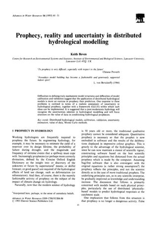
Figure 2 is based on Monte Carlo simulations for a
version of TOPMODEL applied to the Maimai
catchment in New Zealand over a number of storm
events. It is clear from this figure that, although some of
the parameters show some sensitivity to the objective
function (in this case based on the Nash and Sutcliffe31
model efficiency measure) in part of the range
considered, all the parameters have wide ranges in
which different parameter values give equivalent degrees
of fit to the observations. Using the efficiency as the
likelihood measure with a threshold of acceptability for
the simulations of an efficiency of 0.7, the resulting
likelihood weighted uncertainty estimates are shown in
Fig. 3. More detail can be seen for the major event of
lO-
8"
v
4-
.... priori bnd~
o]~lerved
i
0 - m
0 "73 144 216 288 360 432 504 576 648 720 792
time (hours)
Fig. 3. Maimai catchment, 25 May-27 June, storm events. Confidence limits (5 and 95%) for the predictions of the TOPMODEL
calculated using the GLUE procedure in an application to the Maimai catchment in New Zealand. Observed discharges and
simulated prior confidence limits for period 25 May-27 June 1990 are shown with solid and dashed lines respectively.
9. Prophecy, reality and uncertainty in distributed hydrologicalmodelling 49
this record in Fig. 4. It is seen that, with the exception of
the periods around the major peaks, the uncertainty
bands are relatively narrow and bracket the observed
discharges, but that in the periods around the major
peaks, the uncertainty in the discharge predictions
remains high (see particularly Fig. 4, with 90%
confidence limits for the predicted peak flows of
between 4 and 10mm/h). These results are not
untypical of the application of the GLUE methodology
to rainfall-runoff modelling (see also Ref. 5). This
particular period of record was simulated using prior
parameter distributions conditioned on the results of
simulating a number of previous storm periods. Figure 4
also shows the result of using the Bayesian updating
procedure described above to refine the estimates of the
uncertainty limits. In this case, given the conditioning on
previous data sets, there is very little difference in the
prior and posterior confidence limits.
With hydrological systems, of course, it should not
necessarily be expected that the addition of additional
data will decrease the uncertainty in the predictions.
Beven and Binley5 give examples where the posterior
limits, after taking account of the data from the largest
storm in the record, are wider than the prior estimates.
They also show how uncertainty in the input values can
lead to cases where the observed discharges might move
outside the predicted uncertainty limits. It is very
difficult to predict a storm hydrograph if not enough
rainfall appears in the rain-gauge records (see Ref. 20
for an even more extreme example).
One area of interest in the application of the GLUE
technique is the possibility of easily defining likelihood
functions that take account of internal state data, such
as water-table levels, contributing area and soil moisture
patterns, where of course the model structure is capable
of predicting such data directly. In a hypothetical
example, Binley and Beven7 showed that water table
information at a few points in a catchment was not of
great value in refining uncertainty estimates, and that
90% confidence limits for the simulated water tables
were generally at the surface and the base of the
simulated soil! They were making use of a hypothetical
data set based on a three-dimensional Richards equation
simulation of a small basin being simulated by three
two-dimensional planes to represent the catchment
based on the same equation and solver. It appears that
even in this case model structural errors were an
important source of uncertainty in the predictions. It
~6-
v
UO
a~
~4"
8~
I
2.
I
72
.... priori bndJ
observed
....... point.riot bnds
' I
"-~':~ " ' "'"-~>--,D-
I ' I ' I
96 120 144 168
time (hours)
Fig. 4. Maimai catchment, 25 May-27 June, storm events in detail. 28 May 1990. Observed discharges are shown with a solid line,
prior confidence limits with a dashed line and posterior confidence limits after the updating of the likelihood values using data from
this storm period with a dotted line.
10. 50 K. Beven
remains to be seen if similar conclusions will be drawn in
applications to real data. This is currently being
explored for the Maimai and other catchments with
internal state data and will be reported in due course.
7 UNCERTAINTY, MODEL VALIDATION, AND
THE VALUE OF DATA: TOWARDS A POST-
MODERNIST HYDROLOGY
The argument that all hydrological models may be easily
invalidated in catchment-scale applications would
appear to make the notion of model validation
redundant. Yet it would still be useful to be able to
compare the relative merits of different model struc-
tures. Uncertainty estimation provides a methodology
for such a direct comparison through calculation of a
measure of the uncertainty associated with the predic-
tions of each model structure. A number of such
measures are available, including the Shannon entropy
measure (see, for example, Ref. 22). Such uncertainty
measures can be useful in two contexts. In the context of
model validation, they may be used to rank different
model structures, provided that identical likelihood
measures are used in the evaluation of each model.
Uncertainty in observed data and initial and boundary
conditions can also be incorporated into this procedure,
as may well be necessary in hydrological models as
demonstrated by Stephenson and Freeze, 35 and Horn-
berger et al. 2°
A second context that has not received sufficient
attention in the hydrological literature is in assessing the
value of data (but see Refs 12, 15, 16, 24, 34 and 36).
One criterion for the value of additional data in
hydrological simulation is its effect in reducing pre-
dictive uncertainty. In the context of discharge simula-
tion, the availability of a single discharge hydrograph
might have a dramatic effect in reducing the uncertainty
calculated using only the a priori parameter estimates.
Certainly, in the example of the Delphic monkeys, such
data would cause many of the monkeys to revise their
parameter estimates, or the assessors to revise their
previously subjective gradings. But would a discharge
hydrograph be more valuable in reducing the uncer-
tainty associated with a physically-based model than say
the 157 infiltration measurements available to Loague27
in the application of such a model to a small rangeland
catchment?
Geochemical data may also yield additional insights
into hydrological responses, as has been shown, for
example, by the analysis of environmental isotopes.
However, to model such data will require the introduc-
tion of additional parameters, so that there is an
inevitable compromise between the value of additional
data and the identifiability of the parameters required
to take account of that data. Interactions between
parameters is generally such that adding additional
model components may well have repercussions for the
values of parameters in existing model components. The
relationship between parameter identifiability and pre-
dictive uncertainty in the context of hydrogeochemical
models has been discussed by Beck et al.I
One of the aims of this work is to focus attention on
the interaction between data, model structure, para-
meter sets and predictive uncertainty. In the application
of distributed hydrological models there are never
enough data. Thus, invariably, there will be an element
of prophecy about predictions made with the model.
The author would argue that the process of prophecy
needs be examined more carefully in hydrology and that
the hydrologist needs to be realistic about the
uncertainties associated with his prophecies. It may be
that those uncertainties are far greater than we like to
think, if evaluated properly. This is not necessarily a bad
thing. As well as being intellectually honest, it will
highlight the value of appropriate data collection in the
calibration process, uncertainty reduction, and improv-
ing the understanding incorporated into model struc-
tures, including the necessary subjective elements
involved. Certainly, a proposal to evaluate data in
terms of reducing model uncertainty should surely
provide a compelling case for research funding for field
work!
Hydrological prophecy can be considered to be a
trans-scientific activity (see Ref. 33) but the implications
of this have yet to permeate hydrological research and
practice. The outline of a post-modernist hydrology that
recognises the fundamental limitations and subjectivity
of its science has already been presented in the context
of groundwater contamination by Freeze et al. II This
pioneering work has much in common with the aims of
the GLUE methodology developed in the context of
rainfall-runoffmodelling, and indeed goes much further
in incorporating hydrological uncertainty into a full
economic decision analysis framework. The GLUE
procedure provides one easily understood and imple-
mented strategy for addressing some of the problems
inherent in rainfall-runoff modelling. There are
undoubtedly more refined ways of achieving the same
ends. The important thing is that the problems outlined
in this paper be properly recognised and researched in
the future so that, in time, hydrological prophecy can be
given a firmer scientific basis while also explicitly recog-
nising the sociological context in which it takes place.
ACKNOWLEDGEMENTS
The gradual development of the ideas outlined in this
paper has benefitted from discussions from many friends
and colleagues and are being taken further by a group at
Lancaster. Andrew Binley, Renata Romanowicz and
Jim Freer, in particular, deserve thanks. The Maimai
data were provided by Ross Woods of the Freshwater
11. Prophecy, reality and uncertainty in distributed hydrological modelling 51
Research Institute, Christchurch. However, not all of
those friends and colleages will agree with the rather
extreme views presented, and the author would welcome
any comments and weightings awarded for acceptability
(and/or degree of pretentiousness?) from the reader.
This work has been supported in part by NERC grant
GST/02/491 and the ENCORE project of the CEC.
REFERENCES
I. Beck,M.B., Kleissen, F. & Wheater, H.S., Identifying flow
paths in models of surface water acidification. Rev.
Geophys., 28 (1990) 207 30.
2. Beven, K.J., Towards a new paradigm in hydrology. Int.
Assoc. Sci. Hydrol., Pubn. No. 164, (1987) 393-403.
3. Beven, K.J., Changing ideas in hydrology: the case of
physically-based models. J. Hydrol., 105 (1989) 157-72.
4. Beven, K.J., Interflow. In Proc. NATO ARW on
Unsaturated Flow in Hydrological Modelling, ed. H.J.
Morel-Seytoux. Reidel, Dordrecht, 1989, pp. 191-219.
5. Beven, K.J. & Binley, A.M. The future of distributed
models: model calibration and predictive uncertainty.
Hydrol. Process., 6 (1992) 279-98.
6. Beven, K.J. & Kirby, M.J., A physically-based, variable
contributing area model of basin hydrology. Hydrol. Sci.
Bull., 24 (1979) 43 69.
7. Binley, A.M. & Beven, K.J., Physically-based modelling of
catchment hydrology: a likelihood based approach to
reducing predictive uncertainty. In Computer Modelling in
the Environmental Sciences, ed. D.G. Farmer & M.J.
Rycroft. Clarendon Press, Oxford, 1991, pp. 75-88.
8. Binley, A.M., Beven, K.J. & Elgy, J., A physically-based
model of heterogeneous hillslopes. II Effective hydraulic
conductivities. Water Resour. Res., 25 (1989) 1227-33.
9. Binley, A.M., Beven, K.J., Calver, A. & Watts, L.G.,
Changing responses in hydrology: assessing the uncer-
tainty in physically-based predictions. Water Resour. Res.,
27, (1991) 1253-62.
10. Duan~ Q., Sorooshian, S. & Gupta, V., Effective and
efficient global optimisation for conceptual rainfall-runoff
models. Water Resour, Res., 28 (1992) 1015 31.
11. Freeze, R.A., Massmann, J., Smith, L., Sperling, T. &
James, B., Hydrogeological decision analysis: 1. A frame-
work. Ground Water, 28 (1990) 738 66.
12. Freeze, R.A., James, B., Massmann, J., Sperling, T. &
Smith, L., Hydrogeological decision analysis: 4. The
concept of data worth and its use in the development of
site investigation strategies. Ground Water, 30 (1992) 574
88.
13. Gardner, R.H., Huff, D.D., O'Neill, R.V., Mankin, J.B.,
Carney, J. & Jones, J., Application of error analysis to a
marsh hydrology model. Water Resour Res., 16 (1980)
659 64.
14. Garen, D.G. & Burges, S.J., Approximate error bounds
for simulated hydrographs. J. Hydraul. Div. ASCE., 107
(1981) 1519 34.
15. Gates, J.S. & Kisiel, C., Worth of additional data to a
digital computer model of a groundwater basin. Water
Resour. Res., 10 (1974) 1031 8.
16. Gupta, V.K. & Sorooshian, S., The relationship between
data and the precision of parameter estimates of hydro-
logic models. J. Hydrol., 8| (1985) 57.
17. Harlin, J. & Kung, C.-S., Parameter uncertainty and
simulation of design floods in Sweden. J. Hydrol., 137
(1992) 209-30.
18. Hendrickson, J.D., Sorooshian, S. & Brazil, L.E.,
Comparison of Newton-type and Direct Search algo-
rithms for calibration of conceptual rainfall-runoff models.
Water Resour. Res., 24(5) (1988) 691 700.
19. Hornberger, G.M. & Spear, R.C., An approach to the
preliminary analysis of environmental systems. J. Environ.
Manag., 12 (1981) 7-18.
20. Hornberger, G.M., Beven, K.J., Cosby, B.J. & Sapping-
ton, D.E., Shenandoah watershed study: calibration of a
topography-based, variable contributing area model to a
small forested catchment. Water Resour. Res., 21 (1985)
1841 50.
21. Hromadka, T.V. & McCuen, R.H., Uncertainty estimates
for surface runoff'models. Adv. in Water Resour., |1 (1988)
2-14.
22. Klir, G.J. & Folger, T.A., Fuzzy sets, Uncertainty and
Information. Prentice Hall, Englewood Cliffs, 1988.
23. Konikow, L.F. & Bredehoft, J.D. Groundwater models
cannot be validated. Adv. in Water Resour., 15 (1992)75-83.
24. Kuczera, G., Improved parameter inference in catchment
models. 2. Combining different types of hydrologic data
and testing their compatibility. Water Resour. Res., 19
(1983) 1163-72.
25. Kuczera, G., On the validity of first order prediction limits
for conceptual hydrologic models. J. Hydrol., 103 (1988)
229 47.
26. Linstone, H.A. & Turoff, M. (ed.), The Delphi Method:
Techniques and Applications. Addison-Wesley, Reading,
MA, 1975.
27. Loague, K.M., R-5 revisited. 2. Reevaluation of a quasi-
physically-based rainfall runoff model with supplemental
information. Water Resour. Res., 26 (1990) 973 87.
28. Loague, K.M. & Freeze, R.A., A comparison of rainfall-
runoff modelling techniques on small upland catchments.
Water Resour. Res., 21 (1985) 229 40.
29. Melching, C.S., An improved first-order reliability
approach for assessing uncertainties in hydrologic model-
ling. J. ttydrol., 132 (1992) 157 77.
30. Melching, C.S., Yen, B.C. & Wenzel, H.G. Jr., Reliability
estimation in modelling watershed runoff with uncertain-
ties. Water Resour. Res., 26 (1990) 2275-80.
31. Nash, J.E. & Sutcliffe, J.V., River flow forecasting through
conceptual models 1. A discussion of principles. J. Hydrol.,
l0 (1970) 282 90.
32. Nieber, J.L. & Walter, M.F., Two-dimensional soil
moisture flow in a sloping rectangular region: experimen-
tal and numerical studies. Water Resour. Res., 17 (1981)
1722 30.
33. Philip, J.R., Field heterogeneity: some basic issues. Water
Resour. Res., 16 (1980) 443 8.
34. Sorooshian, S., Gupta, V.K. & Fulton, J.L., Evaluation of
maximum likelihood parameter estimation techniques for
conceptual rainfall-runoff models: influence of calibration
data variability and length on model credibility. Water
Resour. Res., 19 (1983) 251 9.
35. Stephenson, G.R. & Freeze, R.A., Mathematical simula-
tion of subsurface flow contributions to snowmelt runoff,
Reynolds Creek watershed, Idaho. Water Resour. Res., |0
(1974) 284--98.
36. Tucciarelli, T. & Pinder, G., Optimal data acquisition
strategy for the development of a transport model for
groundwater remediation. Water Resour. Res., 27 (1991)
577 88.