SlideShare a Scribd company logo
1 of 58
Download to read offline
Mercator Ocean Quarterly Newsletter #36 – January 2010 – Page 1
GIP Mercator Ocean
Quarterly Newsletter
Editorial – January 2010
Figure: 1992-2007 Sea Surface Temperature (ºC) time series in the Nino3.4 Box in the Equatorial Pacific for various Ocean
Reanalyses. MCT2 stands for Mercator Kalman filtering (PSY2G) system reanalysis. MCT3 stands for Mercator 3D-Var reanalysis
(assimilation of altimetry and insitu profiles). SST comparison in all reanalyses shows a relatively robust interannual variability.
SST uncertainty is stable with time. Credits: A. Fischer, CLIVAR/GODAE Ocean Reanalyses Intercomparison Meeting.
Greetings all,
This month’s newsletter is devoted to data assimilation and its application to Ocean Reanalyses.
Brasseur is introducing this newsletter telling us about the history of Ocean Reanalyses, the need for such Reanalyses for
MyOcean users in particular, and the perspective of Ocean Reanalyses coupled with biogeochemistry or regional systems for
example.
Scientific articles about Ocean Reanalyses activities are then displayed as follows: First, Cabanes et al. are presenting CORA, a
new comprehensive and qualified ocean in-situ dataset from 1990 to 2008, developped at the Coriolis Data Centre at IFREMER
and used to build Ocean Reanalyses. A more comprehensive article will be devoted to the CORA dataset in our next April 2010
issue. Then, Remy at Mercator in Toulouse considers large scale decadal Ocean Reanalysis to assess the improvement due to
the variational method data assimilation and show the sensitivity of the estimate to different parameters. She uses a light
configuration system allowing running several long term reanalysis. Third, Ferry et al. present the French Global Ocean
Reanalysis (GLORYS) project which aims at producing eddy resolving global Ocean Reanalyses with different streams spanning
Mercator Ocean Quarterly Newsletter #36 – January 2010 – Page 2
GIP Mercator Ocean
different time periods and using different technical choices. This is a collaboration between Mercator and French research
laboratories, and is a contribution to the European MyOcean project. Then, Masina et al. at CMCC in Italy are presenting the
implementation of data assimilation techniques into global ocean circulation model in order to investigate the role of the ocean on
climate variability and predictability. Fifth, Smith et al. are presenting the Ocean Reanalyses studies at ESSC in the U.K. which
aim at reconstructing water masses variability and ocean transports. Finally, Langlais et al. are giving an example of the various
uses of ocean reanalyses: they are using the Australian BlueLink Reanalysis in order to look into details at the various Southern
Ocean fronts.
The next April 2010 newsletter will introduce a new editorial line with a common newsletter between the Mercator
Ocean Forecasting Center in Toulouse and the Coriolis Data Center at Ifremer in Brest. Some papers will be
dedicated to observations only, when others will display collaborations between the 2 aspects: Observations and
Model. The idea is to wider and complete the subjects treated in our newsletter, as well as to trigger interactions
between observations and modeling communities. This common Mercator-Coriolis Newsletter is a test for which
we will take the opportunity to ask for your feedback.
We wish you a pleasant reading!
Mercator Ocean Quarterly Newsletter #36 – January 2010 – Page 3
GIP Mercator Ocean
Contents
Ocean reanalyses: prospects for multi-scale ocean variability studies .............................................................4
By Pierre Brasseur
CORA -Coriolis Ocean database for Re-Analyses-, a new comprehensive and qualified ocean in-situ dataset
from 1990 to 2008............................................................................................................................................5
By Cécile Cabanes, Clément de Boyer Montégut, Karina Von Schuckmann, Christine Coatanoan, Cécile Pertuisot, Loic Petit de la Villeon, Thierry
Carval, Sylvie Pouliquen and Pierre-Yves Le Traon
Large scale ocean variability estimated from a 3D-Var Reanalysis: sensitivity experiments.............................8
By Elisabeth Remy
Mercator Global Eddy Permitting Ocean Reanalysis GLORYS1V1: Description and Results ............................ 15
By Nicolas Ferry, Laurent Parent, Gilles Garric, Bernard Barnier, Nicolas C. Jourdain and the Mercator Ocean team
Re-analyses in the Global Ocean at CMCC-INGV: Examples and Applications................................................. 28
By Simona Masina, Pierluigi Di Pietro, Andrea Storto, Srdjan Dobricic, Andrea Alessandri, Annalisa Cherchi
Ocean Reanalysis Studies in Reading: Reconstructing Water Mass Variability and Transports....................... 39
By Gregory C. Smith, Dan Bretherton, Alastair Gemmell, Keith Haines, Ruth Mugford, Vladimir Stepanov , Maria Valdivieso and Hao Zuo
Southern Ocean Fronts in the Bluelink Reanalysis.......................................................................................... 50
By Clothilde Langlais, Andreas Schiller and Peter R. Oke
Notebook....................................................................................................................................................... 58
Mercator Ocean Quarterly Newsletter #36 – January 2010 – Page 4
Newsfeature
Ocean reanalyses: prospects for multi-scale ocean variability studies
By Pierre Brasseur
MEOM-LEGI, Grenoble France
Over the past decade, the ocean weather prediction community has made terrific progress toward the establishment of an
effective infrastructure for systematic acquisition and processing of in situ and space observations, assimilation of data into global,
high-resolution ocean circulation models for real-time nowcast and short-range forecast, and delivery of synthetic products to
users. This Operational Oceanography infrastructure represents a unique opportunity for applications that require time series
describing the evolution of ocean state over sufficiently long periods of time (~ 20 to 50 years) to have value for climate research
as well as for regional studies of the ocean variability. The vast majority of ocean weather prediction systems in operation indeed
have the capacity to resolve the whole spectrum of interacting scales from mesoscale eddies to planetary waves, and this is
believed to be a key asset for investigating climate-related modes of the ocean variability.
The application of an ocean weather prediction system to this purpose, however, is neither trivial nor immediate. Structural
changes (e.g. in model resolution, data provision, or assimilation schemes) implemented intermittently in operational suites affect
the accuracy of analyses and make the sequence of estimated ocean states inhomogeneous in quality. As a result, series of 3-D
ocean analyses produced in real-time for nowcast purposes cannot be used for consistent exploration of ocean variability aspects
such as trends and low-frequency signals. Instead, better products can be generated retrospectively by re-analysing past
observations with a fixed ocean model and a fixed data assimilation scheme in which the best available parameterizations and
assimilation options have been prescribed. A retrospective analysis, or reanalysis, offers the possibility of extracting additional
information from data sets generated a posteriori with improved reprocessing algorithms. Reanalyses can therefore contribute to
more confident attribution of the processes that are responsible for the observed variability as well as the expected geographical
patterns and magnitudes of the responses. In return, reanalysis products could ultimately provide relevant information on how to
design appropriate observing systems and optimized sampling strategies for the ocean, especially for the detection of climate
variability signals. Dedicated Observation Sensitivity Experiments (OSEs) for instance, can provide information about the
sensitivity of reanalyses to the density of the observation network.
In essence, the systems that are producing 4-D historical reconstructions should be different from those used in real-time. An
obvious difference when operating an assimilation system in retrospective mode lies in the possibility of using both “past” and
“future” observations. This motivates the development of new assimilation algorithms, such as Kalman-type smoothers that, in the
future, should supersede the Kalman-type filters currently available in most operational centers.
Another fundamental difference between a reanalysis and a raw sequence of ocean state estimations produced at discrete time
intervals lies in the “dynamical” dimension, which should be very carefully taken into account for the reconstruction of 4-D fields.
The dynamical constraints imposed by physical laws are critical for inferring unobserved quantities such as currents, or to
compute transport of tracers and integrated circulations through sections. To some extent however, the requirement for dynamical
consistency over periods of time larger than the predictability time scales of the simulated flow remains an issue at conceptual
level. This is especially true with eddy-resolving ocean models for which the so-called “weak-constraint” assimilation methods (i.e.
assuming that the model equations are not strictly verified) represent the relevant framework to properly conciliate imperfect
models with imperfect data.
Other key challenges will have to be addressed in the future, such as reanalyses with coupled components of the ocean-
atmosphere-biosphere system and the need for consistent uncertainty estimates on the solutions. Ensemble methods are already
being implemented for nowcast and short–term predictions, and provide an elegant and powerful statistical methodology to
quantify uncertainty. However, running ensembles of statistical significance still represent a major computational issue with regard
to the production of multi-decadal data sets. The same difficulty exists for variational assimilation methods, as in this case the
error estimation process requires the computation of the inverse of the Hessian of the cost function.
The reanalysis concept has been proven first in the atmosphere in the eighties, and atmospheric reanalyses have become an
essential by-product of major numerical weather prediction systems. In oceanography, reanalyses of the global ocean/sea-ice
system have already been produced under the auspices of GODAE and CLIVAR, leading to intercomparison exercises
coordinated at international level. Today, the production and delivery of ocean reanalyses is identified as a major task for the
future Marine Core Services of GMES. In the framework of the EU-funded MyOcean project, several monitoring and forecasting
centers (Mercator, INGV, MetNo …) are committed to provide qualified reanalyses to users from different applicative sectors
(climate, seasonal and weather forecasting, management of marine resources, coastal environment monitoring and assessment).
No doubt that users will be increasingly demanding in terms of quality and validation of products, and this will represent a very
significant driver for the whole Operational Oceanography community in the next decade.
Mercator Ocean Quarterly Newsletter #36 – January 2010 – Page 5
CORA -Coriolis Ocean database for Re-Analyses-, a new comprehensive and qualified ocean in-situ dataset from 1990 to 2008
CORA -Coriolis Ocean database for Re-Analyses-, a new comprehensive
and qualified ocean in-situ dataset from 1990 to 2008
By Cécile Cabanes
1
, Clément de Boyer Montégut
1
, Karina Von Schuckmann
1
, Christine
Coatanoan
2
, Cécile Pertuisot
2
, Loic Petit de la Villeon
2
, Thierry Carval
2
, Sylvie Pouliquen
1
and
Pierre-Yves Le Traon
1
1
Laboratory of Oceanography from Space (LOS), IFREMER/CNRS, Brest, France
2
Coriolis Data Centre, IFREMER, Brest, France
Introduction
An ideal set of oceanographic data would comprehends a global coverage, continuity in time, is subject to regular quality controls
and calibration processes (i.e. durable in time), and encompasses several space/time scales. This goal is actually not easy to
reach and reality is often different especially with in-situ oceanographic data, such as temperature and salinity profiles in our case.
Those data have basically as many origins as there are scientific campaigns to collect them. Some efforts to make such an ideal
dataset have been done for many years, especially since the initiative of Levitus (1982).
A program named Coriolis has been set up at Ifremer data centre the beginning of the 2000's in the wake of the development of
operational oceanography in France. The project was launched in order to contribute to the ocean in situ measurements part of
the French operational system (e.g. Mercator group). It has been especially involved in developing continuous, automatic, and
permanent observation networks. The data centre is gathering ocean data in real time, which are then subject to its own quality
procedures (Coatanoan and Petit de la Villéon, 2005). Our goal now is to distribute an extraction of this comprehensive and
reprocessed set of ocean in-situ data, from 1990 to 2008. The aim is to publish this qualified dataset for operational as well as for
research purposes. In doing this work, we can also evaluate the difference between our dataset and state of the art databases like
the World Ocean Database 2009 (Boyer et al, 2009) for example. This is also a way to improve the quality of this “living” real time
database. We first present a description of the dataset and of the quality controls applied, then we give examples of the main uses
for which those data are meant for.
Description of the Dataset
Overview
The CORA dataset basically contains global, sub-surface ocean profiles of in-situ temperature and salinity at observed
levels. Those data were extracted from the real-time CORIOLIS database at the beginning of 2008 (and early 2009 for 2008 data).
From those raw data, we construct and make available profiles data at standardized levels, and gridded fields of T/S obtained
through objective analysis.
Data type
CORA contains data from different types of instruments: mainly Argo floats, XBT, CTD and XCTD, and Mooring Data (see figure
1). The Coriolis centre receives data from Argo program, French research ships, GTS data, GTSPP, GOSUD, MEDS, voluntary
observing and merchants ships, moorings, and the World Ocean Database (not in real time for the last one).
Quality controls
To produce this dataset, several tests have been developed in order to improve the quality flags of the raw database and to fit the
level required by the physical ocean re-analysis activities. These tests include some simple systematic tests, a test against
climatology and a more elaborate statistical test involving an objective analysis method (see Gaillard et al., 2009 for further
details). Visual quality control (QC) is performed on all the suspicious temperature (T) and salinity (S) profiles. The statistical test
is based on an objective analysis run with a three weeks window in order to capture the most doubtful profiles. They are then
visually checked by an operator who decides whether or not they are bad data or real oceanic phenomena. Then a second run
which takes into account only the good data is operated on a one week window in order to produce the gridded fields. Each
release provides T and S gridded fields and individual profiles both on their original levels and interpolated levels.
Mercator Ocean Quarterly Newsletter #36 – January 2010 – Page 6
CORA -Coriolis Ocean database for Re-Analyse-, a new comprehensive and qualified ocean in-situ dataset from 1990 to 2008
Figure 1
Temporal (left) and spatial distribution in 2007 (right) for the different type of data used in CORA.
Goals and uses of the Dataset
Research
CORA database is meant to investigate specific scientific questions. Achieving this goal will lead to the improvement of the quality
of the dataset, by detecting abnormal data especially. That will benefit subsequently to the data centre real-time database and the
operational results. It is also a way to monitor ocean variability as it is done on the framework of the MyOcean European project
(http://www.myocean.eu.org/).
This dataset can be used to estimate the change in global ocean temperature and heat content during the 2003-2008 time period.
As shown in previous results, the world ocean is warming (e.g. Levitus et al., 2005). The work of von Schukmann et al. (2009)
shows that the signal propagates to increasing depth in time, especially in the northern hemisphere. The average warming rate is
0.77 ± 0.11 W/m2 for the 0-2000m depth layer during 2003-2008.
Ocean model validations
CORA can be used to construct elaborated products such as climatologies of heat content, depth of the thermocline or 20°C
isotherms, or indexes (niño3.4, MOC, PDO…). Such products are especially useful for validating ocean model outputs and
improve their quality or assess their results. For example, de Boyer Montégut et al. (2007) validates their OGCM mixed layer
depth outputs against in-situ observations in the northern Indian Ocean. After assessing the realism of their experience, they use
the model to investigate surface heat budget variability.
Assimilation in ocean models
An important application of such a database is also for ocean model assimilation projects. In France, the goal of GLORYS (GLobal
Ocean ReanalYsis and Simulations) project is to produce a series of realistic eddy resolving global ocean reanalyses. Several
reanalyses are planned, with different streams. Each stream can be produced several times with different technical and scientific
choices. Version 1 of Stream 1 (GLORYS1V1) is produced using the previous version of the CORA data set (see Ferry et al, this
issue) and is available on request from products@mercator-ocean.fr. The ocean general circulation model used is based on
ORCA025 NEMO OGCM configuration (Barnier et al., 2006).
Mercator Ocean Quarterly Newsletter #36 – January 2010 – Page 7
CORA -Coriolis Ocean database for Re-Analyse-, a new comprehensive and qualified ocean in-situ dataset from 1990 to 2008
Références
Barnier B., G. Madec, T. Penduff, J.-M. Molines, A.-M. Treguier, J. Le Sommer, A. Beckmann, A. Biastoch, C. Böning, J. Dengg,
C. Derval, E. Durand, S. Gulev, E. Remy, C. Talandier, S. Theetten, M. Maltrud, J. McClean and B. De Cuevas et al., 2006:
Impact of partial steps and momentum advection schemes in a global ocean circulation model at eddy permitting resolution.
Ocean Dynamics, DOI: 10.1007/s10236-006-0082-1.
Boyer T.P., J. I. Antonov, O. K. Baranova, H. E. Garcia, D. R. Johnson, R. A. Locarnini, A. V. Mishonov, D. Seidov, I. V. Smolyar,
and M. M. Zweng, 2009: World Ocean Database 2009, Chapter 1: Introduction, NOAA Atlas NESDIS 66, Ed. S. Levitus, U.S. Gov.
Printing Office, Wash., D.C. , 216 pp., DVD.
de Boyer Montégut, C., J. Vialard, S. S. C. Shenoi, D. Shankar, F. Durand, C. Ethé, and G. Madec, 2007,:Simulated seasonal and
interannual variability of mixed layer heat budget in the northern Indian Ocean, J. Climate, 20, 3249-3268
Coatanoan C., and L. Petit de la Villéon, 2005: Coriolis Data Centre, In-situ data quality control procedures, Ifremer report, 17 pp.
(http://www.coriolis.eu.org/cdc/quality_control.htm)
Gaillard F., E. Autret, V. Thierry, P. Galaup, C. Coatanoan, and T. Loubrieu, 2009: Quality controls of largeArgo datasets, J.
Atmos. Ocean. Tech., 26, 337-351
Levitus, S., 1982: Climatological Atlas of the World Ocean, NOAA Professional Paper 13, U.S. Government Printing Office,
Rockville, M.D., 190 pp.
Levitus, S., J. Antonov, and T. Boyer, 2005: Warming of the world ocean, 1955-2003, Geophys. Res. Lett., 32.
von Schukmann, K., F. Gaillard and P.Y. Le Traon, 2009: Global hydrographic variability patterns during 2003-2008, J. Geophys.
Res.
Mercator Ocean Quarterly Newsletter #36 – January 2010 – Page 8
Large scale ocean variability estimated from a 3D-Var Reanalysis at Mercator: sensitivity experiments
Large Scale Ocean Variability Estimated from a 3D-Var Reanalysis at
Mercator: Sensitivity Experiments
By Elisabeth Remy
1,2
1
CERFACS, Toulouse, France
2
MERCATOR-OCEAN, Toulouse, France
Introduction
Ocean reanalysis aims at combining available observations with a general circulation model (GCM) to provide a more accurate
description of the historical ocean state than can be obtained by model or observations alone. In this context, the model can be
interpreted as a space-time dynamical interpolator of the observations. Here we consider a large scale decadal ocean reanalysis
that has been produced by combining in situ and altimeter observations with a global ocean GCM using a three-dimensional
variational (3D-Var) approach. Our objective is to assess the improvement brought by data assimilation and to illustrate the
sensitivity of the ocean state estimates to different assimilation configurations. We focus on the large scale interannual variability.
Model configuration
The ocean model is the LOCEAN primitive equation model OPA8.2 (Madec et al., 1998) in its low resolution configuration
ORCA2°. The version of the model used here is a fre e-surface constant volume configuration. Atmospheric forcing fields are
applied as “forced flux”. They are derived from the ECMWF atmospheric reanalysis ERA40. After year 2001 when ERA40 is not
available, they are taken from ECMWF operational analyses. A strong restoring term to the weekly Reynolds SST is applied, with
a coefficient of 200W/m2. The ERA precipitation field has been bias corrected using GPCP precipitation data (Troccoli and
Källberg, 2004).
As the global water mass budget is not closed due to large errors in the fresh water fluxes, an additional constraint is applied to
close the budget. As a consequence, the model is unable to represent that part of the eustatic trend due to atmospheric mass
input observed in altimeter observations.
Variational assimilation method / code
The assimilation system is based on the OPAVAR system developed at CERFACS. The model configuration and assimilation
parameters are very close to the setup of the ENSEMBLE experiments. A detailed description of the assimilation system and
reanalysis procedure can be found in Daget et al. (2009). The major difference with our system is that we assimilate along track
Sea Level Anomalies.
Here we quickly recall the basis of the variational approach. The 4dvar method is based on minimization of a cost function which
contains the square root of the observation misfits and a priori information on the solution. The minimum, x*, is a model trajectory
close to the observations in agreement with the prescribed model and observation errors. The problem to solve can be expressed
as follows:
x* as J(x*)=min(J(x)), (eq. 1)
x verifying the model equation : xi+1=M(xi)
where : J(x) = ½ [x0-x0
b
] T
B-1
[x0-xb0
b
] + ½ Σ[H(xi) – yo
]T
R-1
[H(xi) – yo
] (eq. 2)
Here we search the optimal initial conditions, x0.
- x0 is the control vector we want to estimate: it contains the uncorrelated model state variable, x0
b
is the background
estimate, usually taken as the final state of the previous assimilation cycle,
- B is the background model error covariance matrix,
- yo
observation vector,
- R is the observation error covariance matrix
This minimization of the cost function is done iteratively using a descent algorithm: at each iteration the gradient is used to
compute a new correction in the direction of the minimum. This allows taking into account the non linearity of the model equations.
Mercator Ocean Quarterly Newsletter #36 – January 2010 – Page 9
Large scale ocean variability estimated from a 3D-Var Reanalysis at Mercator: sensitivity experiments
The 3dvar FGAT (First Guess at Appropriate Time) is derived from the incremental formulation of the 4Dvar. In the 3dVar FGAT
approximation, the cost function is linearized and the gradient to compute the descent direction is approximated. The innovation,
yo-H(xib), is computed at the observation time. The method is described in Weaver et al. (2003,2005).
The assimilation window for the experiment presented here is 10 days.
The background error covariance matrix, B, contains the variance of the model error on the diagonal, covariance terms and spatial
correlation specification off diagonal. The standard deviation prescribed for each control variable depends on the current state of
the ocean. The multivariate relations link the model variables using dynamical or physical relationships between the variables. For
example, the “salinity balance operator” (Ricci et al, 2005) preserves the water mass properties, insuring that salinity varies
according to temperature changes, even without any salinity data assimilated. First order physical equilibrium are also prescribed
between the other variables, as the geostrophic equilibrium for velocity, steric component for the sea level.
Observations
Before assimilating observations, it is important to understand their information content, the data processing, and possible filtering,
subsampling, in order to precisely compute their equivalent with the model variables and the error estimate.
In situ profiles : observation data sets
For the experiments described here we used the quality-controlled ENSEMBLES (EN3 v1a) in situ dataset produced at the Met
Office. Details on the databases used to construct it and the quality control checks that were applied can be found on the
dedicated webpage (http://hadobs.metoffice.com/en3/) and in the article by Ingleby and Huddleston (2007).
Sea level anomaly data
The dynamic topography reflects the elevation of sea level due to ocean currents, the steric expansion of the water, and mass
forcing from land and atmosphere. It can be defined as the sum of a time mean, the so called Mean Dynamic Topography (MDT)
and time variations about this mean: Sea Level Anomalies (SLA). Satellite altimeters estimate the distance to the sea surface,
providing accurately the variations of the sea surface. Important pre-treatment of the data are done in order to correct this distance
from propagation error in the atmosphere, tides, etc... Along track SLA are assimilated. A delayed time product from AVISO is
chosen due to a higher quality of the post processing and its homogeneity over the time period.
The observation error covariance matrix, R, is diagonal. It represents the confidence interval given to the observation compared to
its model equivalent. It takes into account not only the measurement error but also the representativity error. The measurement
error can contain an instrument error and treatment error, as the representivity error contains signals viewed by observations but
not represented by the model. This part of the error can be dominant especially with low spatial resolution model like ORCA2. The
model is not able to represent explicitly the mesoscale activity, sharp fronts, etc…
The estimation of the representativity error is based on the statistical approach (Fu et al, 1993) under the hypothesis of
uncorrelated observation error. The underlying assumption is that the representativity error can be computed using the variance of
the observations compared to the variance of the model. Figure 1 shows the representativity error estimated for the in situ
temperature observations and along track sea level anomalies.
Figure 1
Representativity error maps for temperature observations (longitudinal mean for the global ocean) in °C and along track sea level
anomalies in mm.
Mercator Ocean Quarterly Newsletter #36 – January 2010 – Page 10
Large scale ocean variability estimated from a 3D-Var Reanalysis at Mercator: sensitivity experiments
Experiment setup
We define a default experiment covering the period 1960-2005 using the available observations, in situ and SLA referenced to the
model MDT. The model counter part of the observations is computed at the nearest time step. For moored buoy data (e.g., TAO),
the model equivalent is a daily mean model temperature field. In space, the model counterpart is computed with an interpolation
from the model grid to the observation point.
Different experiments were also done to test the sensitivity of the estimated ocean circulation to the MDT and the type of
assimilated observations. The table 1 summarizes the setup of those experiments.
Time frame In situ observations SLA observations
Control 1960-2005 No No
b090 1960-1992 Yes No
b09a 1993-2005 Yes No
b09b 1993-2005 Yes Yes + Model MDT
b09c 1993-2005 Yes Yes + Rio MDT
Table 1
Experiments setup
To follow the global sea level rise observed from altimetry measurements, we let the global mean sea level in the model adjust
freely. Note that theoretically, the correct approach would be to remove from the SLA observations this signal that the model is not
able to properly represent: the global mass budget is forced to zero in the model and the model is built with a volume conservation
hypothesis.
Sensitivity experiments
The sensitivity of the linear trend of different diagnosed quantities is presented here. We focus on the period 1993-2001 where we
compare the trends estimated from the model with the trend estimated from observations. In experiment b09a only in situ
observations are assimilated, while in b09b and b09c, SLA observations are assimilated in addition. The MDT used in the b09b
experiment is the model MDT computed from the control model simulation whereas in b09c it is the Rio MDT (Rio and Hernandez,
2004) (Table 1). Estimates of the 0-300 meter mean temperature, salinity and sea level linear trends are presented in Figure 2.
We compare the temperature estimation to monthly objectively analyzed subsurface temperature by Ishii et al.(2003) The analysis
is based on different datasets including the World Ocean Database/Atlas.
Globally, one can see very similar estimates of the mean temperature trend over the first 300 meters in the different assimilation
experiments, comparable to the observed trend. This robustness can be attributed to the data density which allows controlling this
variable. In the Southern ocean were data are very sparse, solutions slightly differ. The observations analysis, done by Ishii et al.
(2003), does not show significant trend in this region.
The salinity trend appears to be extremely sensitive and strongly differs between experiments. Unrealistically strong trends appear
in the southern hemisphere when altimeter data are assimilated. The trend is even stronger when the Rio MDT is used.
The sea level trend is already well constrained by the in situ observations. The assimilation of altimeter data improves the
amplitude. The trend is then very close to the observed one for whichever MDT is chosen.
To understand these results, we note that both in situ and SLA observations contain information on the temperature and salinity
field. The in situ data provide direct information through T and S profiles, whereas the sea level data (MDT+SLA) reflect the heat
and haline content over the whole water column due to the sea water expansion. A hypothesis is that the salinity tends to
compensate the inconsistency between the dynamic height deduced from the MDT+SLA and from the in situ observations due to
the use of different MDTs compared to the real one. The northern hemisphere is less sensitive probably due to a larger amount of
salinity data in this region.
For all these diagnostics, the simulation without assimilation shows the right large scale patterns but with unrealistically small
amplitudes: the impact of the assimilation is clearly positive in this respect.
Mercator Ocean Quarterly Newsletter #36 – January 2010 – Page 11
Large scale ocean variability estimated from a 3D-Var Reanalysis at Mercator: sensitivity experiments
0-300 m temperature trend (°C) 0-300 salinity trend
(PSU)
Sea Level trend
(m)
controlrunInsitu(b09a)Insitu;SLA+model
MDT(b09b)MDT
Insitu;SLA+RioMDT
(b09c)
Observationanalysis
Ishii analysis
AVISO maps
Figure 2
1993-2001 0-300 m temperature (°C), salinity (PSU) and sea level (m) linear trend from assimilation experiments and from
analysis of observations
Analysis of the reference simulation 1960-2005
We illustrate the reanalysis results with a few diagnostics focusing on the subsurface representation of the ocean interannual
variability estimated from the experiments b090 and b09b over the period 1960-2005 (Table 1). The large increase of the number
of in situ observations at the beginning of the ARGO era improves the control of the ocean model variables: the mean misfit to the
in situ observations is significantly reduced from 1960 to 2005, especially between 300 and 700 meters depth (not shown here).
Temperature, salinity and SSH trend
The temperature linear trend from 1960 to 2005 is clearly non uniform (Figure 3, left panel). The North Atlantic is warming, as the
Pacific is cooling in the subtropical gyre and warming in the southern part. The vertical mean profile temperature evolution for the
North East Atlantic (box shown on the temperature trend map) is presented on the right. Mode water formation occurs in this
Mercator Ocean Quarterly Newsletter #36 – January 2010 – Page 12
Large scale ocean variability estimated from a 3D-Var Reanalysis at Mercator: sensitivity experiments
region of subduction. Successive warm and cold signals propagate from the surface to deeper layers. This clearly shows the
importance of the long term variability in the ocean. The situation is very different depending on the region we look at.
Figure 3
Mean 0-300 m temperature trend 1960-2005 on the left and mean temperature vertical profile evolution in the north east Atlantic
(box on the left map) on the right, in °C.
Figure 4 represents the estimated linear trend of the sea level rise on the left and the dynamic height on the right. The Atlantic
Ocean shows a rising sea level in the middle of the subtropical gyres, whereas the Pacific Ocean shows different tendencies
depending on the latitude. The dynamical height reflects the steric part of the sea level. The differences with the sea level are due
to mass changes: advection or input from land, including ice cap or atmosphere. They appear mainly in the southern Pacific
Ocean and the Indian Ocean. The partition of the SLA into an eustatic and a steric contribution (dynamic height) is sensitive to the
specification of the background error covariance between the different model variables in B (eq. 2). The full model description of
the ocean state allows us to decompose the dynamic height into its thermosteric and halosteric part. Those components (not
shown here) have opposite contributions: the halosteric tends to moderate the thermosteric part which has an even higher trend
than the total dynamical height.
Figure 4
Sea level (left) and dynamical height (right) linear trend from 1960 to 2005 in meters.
Interannual variability
Up to now we have looked at the linear trend, while here we illustrate the use of the reanalysis to examine the interannual
variability. A projection on Empirical Orthogonal Functions (EOF) gives an interesting way to analyse the variability of the ocean
circulation. The modest size of the model state vector in ORCA2 allows us to perform this computation easily on the 45 years of
the simulation.
Figure 5 shows the different spatial patterns associated with the first 3 EOFs of the mean temperature over 0-300m. The EOF
coefficient time series is also presented. The seasonal signal has been removed. The ENSO pattern is largely dominant and
corresponds to the 1st EOF which explains 26% of the variance. The balance between the eastern and western part represents
the change of the slope of the thermocline. The link with the Indian Ocean also clearly appears. The signal in the Atlantic is too
small to be significant. The second EOF is also mainly related to tropical Pacific dynamics, while in the Atlantic Ocean a quasi-
uniform pattern exists. The third EOF looks like the warming trend, especially in the Atlantic Ocean. The fourth panel of Figure 5
Mercator Ocean Quarterly Newsletter #36 – January 2010 – Page 13
Large scale ocean variability estimated from a 3D-Var Reanalysis at Mercator: sensitivity experiments
shows the time evolution of the coefficients of the 1st three EOFs. The red curve corresponds to the first EOF, the green one to
the second EOF, and the blue one to the third EOF.
Figure 5
First three EOFS of the decomposition of the mean 0-300m temperature and the time series of the coefficients from 1960 to 2005
(1st
eof in red, second in green, third in blue).
Conclusion
This study shows that even with a low resolution ocean model, the large scale variability of the upper ocean can be effectively
constrained by assimilating in situ profiles and sea level observations. Some estimates are robust and close to the observed one;
others appear to be more sensitive, like salinity. The low resolution configuration provides a useful tool for sensitivity experiments
which are too expensive with high resolution models. The comparison of the reanalysis results with the forced run without
assimilation shows a significant improvement in the amplitude of the variability of the upper ocean temperature field. The
MERCATOR Glorys reanalysis is based on the ORCA ¼° global configuration and the SAM2 assimilation scheme using local
inversions. It will be interesting to test the control of the large scale with this 3D-Var complementary to the local analysis method.
Acknowledgements
I would like to thank Anthony Weaver for his comments on this article.
References
Fu L.L., I. Fukumori, and R.N. Miller, 1993: Fitting dynamic models to the geosat sea level observations in the tropical Pacific
Ocean. part ii : A linear, wind-driven model. Journal of Physical Oceanography, 23, p. 2162-2181.
Ingleby, B., and M. Huddleston, 2007: Quality control of ocean temperature and salinity profiles - historical and real-time data.
Journal of Marine Systems, 65, 158-175.
Ishii, M., M. Kimoto, M. Kachi, 2003: Historical Ocean Subsurface Temperature Analysis with Error Estimates, Monthly Weather
Review, Vol. 131, Issue 1, p. 51-73.
Madec, G., P. Delecluse, M. Imbard and C. Levy, 1998: OPA 8.1 Ocean General Circulation Model reference manual. Tech. rep.,
Institut. Pierre-Simon Laplace (IPSL), France, No11, 91pp.
Ricci S., A. T. Weaver, J. Vialard, P. Rogel, 2005: Incorporating State-Dependent Temperature–Salinity Constraints in the
Background Error Covariance of Variational Ocean Data Assimilation, Monthly Weather Review, Vol. 133, Issue 1, p. 317-338.
Mercator Ocean Quarterly Newsletter #36 – January 2010 – Page 14
Large scale ocean variability estimated from a 3D-Var Reanalysis at Mercator: sensitivity experiments
Rio, M.-H., and F. Hernandez, 2004: A mean dynamic topography computed over the world ocean from altimetry, in situ
measurements, and a geoid model, J. Geophys. Res., 109, C12032.
Weaver A. T, J Vialard, and D. L. T Anderson, 2003: Three- and four-dimensional variational assimilation with a general circulation
model of the tropical Pacific Ocean. Part I: Formulation, internal diagnostics, and consistency checks. Mon. Wea. Rev., 131,
1360–1378.
Mercator Ocean Quarterly Newsletter #36 – January 2010 – Page 15
Mercator Global Eddy Permitting Ocean Reanalysis GLORYS1V1 : Description and Results
Mercator Global Eddy Permitting Ocean Reanalysis GLORYS1V1:
Description and Results
By Nicolas Ferry1
, Laurent Parent1
, Gilles Garric1
, Bernard Barnier2
, Nicolas C. Jourdain2
and
the Mercator Ocean team.
1
Mercator Océan, Ramonville St Agne, France
2
MEOM-LEGI, CNRS, Université de Grenoble, Grenoble, France
Abstract
We present here preliminary results from the French Global Ocean Reanalysis and Simulations (GLORYS) project which aims at
producing a series of global ocean reanalyses. This project is a collaboration between Mercator-Ocean and French research
laboratories, and is a contribution to the project of the European Union MyOcean. The overall objective is to produce state of the
art eddy resolving global ocean simulations constrained by oceanic observations by means of data assimilation. GLORYS plans to
produce different streams, spanning different time periods and using different technical choices. Here, we present GLORYS1V1
(the first version of the stream 1 reanalysis) covering the “Argo” era (2002-2008), a period characterized by its unique high density
of remotely sensed and in situ observations. Assimilation diagnostics as well as the evaluation of the representation of some
circulation features are presented.
Introduction
In the last decade, real-time high-resolution ocean analysis and forecasting have become routine tasks done by several
operational centers throughout the world (Dombrowsky et al. 2009). Downstream applications of these near real-time operational
analyses and forecasts have been demonstrated in many areas such as marine pollution monitoring (Hackett et al. 2009) and
marine safety (Davidson et al. 2009), coastal modelling (De Mey et al. 2009), ocean initialization for seasonal forecasting
(Balmaseda et al. 2009), support to the navies (Jacobs et al. 2009), biochemistry modeling (Brasseur et al. 2009) etc. Some
specific applications of ocean state estimation however require long time series of the three dimensional ocean state called ocean
reanalyses. Several groups have produced in the last years ocean reanalyses spanning, for the longest one, the 1960-present
time period (Lee et al. 2009). This kind of product is used mostly for climate research, (Lee at al. 2009), for long coupled ocean-
atmosphere hindcasts for seasonal forecasts (Balmaseda et al. 2009), and helps to the building of new climate indicators for
coastal upwelling, precipitation and extreme weather events such as tropical storms and cyclones (Xue et al. 2009).
Most of the ocean reanalyses are available at coarse resolution (Rienecker et al. 2009) with a horizontal resolution of ~1°and do
not include explicitly the mesoscale effects in the estimation of the ocean state. This means that during the altimetric years (1992-
present) the observed eddy variability and its subsequent effects (e.g. eddy induced transports) may not be properly taken into
account. Another reason why higher resolution reanalyses should be carried out is that fronts (associated to western boundary
currents for example) are better resolved and regional biases (like the Gulf Stream overshoot) are reduced. Lastly, high resolution
reanalyses should also be beneficial for downstream applications of like biogeochemical modelling or regional / coastal modelling.
With its experience in the field of ocean analysis and forecasting, Mercator has developed a global ocean eddy permitting
resolution (1/4°) reanalysis system. This work is d one in the framework of the French GLobal Ocean ReanalYsis and Simulations
(GLORYS) and the EU funded MyOcean projects. The objective is to produce a series of realistic (i.e. close to the existing
observations and consistent with the physical ocean) eddy resolving global ocean reanalyses. Here we present the stream 1
reanalysis (called GLORYS1V1) spanning the 2002-2008 time period (the “Argo” era). The reanalysis system is similar in many
aspects to the Mercator operational ¼° global ocean analysis/prediction system (Dombrowsky et al. 2009). However,
GLORYS1V1 benefits from significant improvements that are presented here. This paper describes the way Mercator operational
¼°global ocean analysis / forecast system has been modified to produce a 7-year reanalysis. Then, the results of the reanalysis
are presented and compared to the operational system in 2007-2008.
Description of GLORYS1V1 reanalysis system
The ocean reanalysis system used (called GLORYS1V1) is based on the operational system PSY3V2 used at Mercator1.
GLORYS1V1 benefits from several improvements that we present in the following section. We describe the different components,
namely the ocean/sea-ice model, the data assimilation method, the ocean initialization and the observations assimilated. We also
1
(http://bulletin.mercator-ocean.fr/html/produits/psy3v2/psy3v2_courant_en.jsp)
Mercator Ocean Quarterly Newsletter #36 – January 2010 – Page 16
Mercator Global Permitting Ocean Reanalysis GLORYS1V1 : Description and Results
carefully review the improvements with respect to the operational system. Table 1 summarizes the main differences between the
operational system PSY3V2 and GLORYS1V1. The starting date of GLORYS1V1 simulation is 3 October 2001.
Ocean-sea ice model
The model configuration is the same as the one used in the operational global ocean system operated in near real time at
Mercator since November 2005 (Drevillon et al. 2008a, Drevillon et al. 2008b). It is a global implementation of the ocean/sea-ice
NEMO numerical framework (version 1.09, Madec, 2008) and has many common features with the ORCA025 configuration
developed by the European DRAKKAR collaboration (Drakkar group, 2007), the numerical details of which are given in Barnier et
al. (2006). The ocean model component is the free surface, primitive equation ocean general circulation model developed at
LOCEAN (Madec, 2008). The sea-ice component is the LIM2 sea-ice model (Goosse and Fichefet, 1999). The geographical
domain extends from -77°S to the North Pole. The ve rtical discretisation uses partial steps with 50 vertical levels with an
increased resolution near the surface (~1 m near the surface, 11 levels over the top 15m, 500 m at depth). Compared to the
operational system PSY3V2, the sea-ice model used for GLORYS1V1 benefits from the following improvements: (i) an Elastic
Viscous Plastic (EVP) dynamics of the ice and (ii) a computation at each time step of the ocean-ice stress. These two new
parameterizations improve clearly the results of the ice model, in particular the ice extent during summer in the Arctic Ocean
(Garric et al., 2008). This improved ice model version is referred to as LIM2_EVP. The CLIO bulk formula (Goose et al., 2001) are
used in both GLORYS1V1 and the operational system to calculate the atmospheric forcing function. They are fed with surface
variables from ECMWF operational analyses (1-day averages). The ECMWF precipitation field is corrected using GPCP monthly
data (Garric, 2006) in a way similar to that proposed by Troccoli and Källberg (2004). This correction is however not sufficient to
constrain the global average water budget (evaporation, precipitation and runoff) to a realistic value. That is why the global water
budget is set to zero at each time step. Initial conditions used for the ocean are derived from the ARIVO climatology (Gaillard et al.
2008, Gaillard and Charraudeau, 2008) for the month of October. The sea ice initial condition is the sea ice state in October 2001
from a multi decadal model integration performed by the DRAKKAR group (namely G70, Drakkar Group 2007) with the same
ocean-sea-ice model.
Data assimilation method
The data assimilation method developed at Mercator (Tranchant et al. 2008) is used in GLORYS1V1. The assimilation scheme is
an extended Kalman filter based on the SEEK approach developed at LEGI (e.g. Testut et al. 2003). This approach is used since
several years at Mercator and has been implemented in different ocean model configurations like the PSY3V2 1/4°global ocean
operational analysis forecasting system.
The SEEK formulation requires knowledge of the forecast error covariance of the control vector. In GLORYS1V1, this vector is
composed of the barotropic height field and the 3-dimensional temperature, salinity, zonal and meridional velocity fields. The
forecast error covariance is based on the statistics of a collection of ocean state anomalies (typically ~300) and is seasonally
dependent. This approach comes from the concept of statistical ensembles where an ensemble of anomalies is representative of
the error covariances (ergodic theory). This approach is similar to the Ensemble Optimal Interpolation (EnOI) developed by Oke et
al. (2008) which is an approximation to the EnKF (Ensemble Kalman Filter) that uses a stationary ensemble to define background
error covariances. In our case, the anomalies are high pass filtered ocean states available over the 1992-2001 time period. It
should be noted that the analysis increment is a linear combination of these error modes and depends on the model innovation
(observation-model misfit) and on the observation errors.
The length of the assimilation cycle is 7 days and the data assimilation produces,, after each analysis, global increments for the
ocean barotropic height, temperature, salinity, zonal and meridional velocity. An Incremental Analysis Update (IAU) method
(Bloom et al. 1996) is used to apply the increment to reduce the spin up effects after the analysis time. We implemented the IAU
variant described in Benkiran and Greiner (2008) where each analysis increment is applied during two assimilation cycles: the one
before and the one after the analysis time.
Observations
The assimilated observations consist in Sea Surface Temperature (SST) maps, along track sea level anomaly (SLA) data, and in
situ temperature and salinity profiles. The SST comes from the daily NCEP RTG 1/2°product (Thiébaux, 2003) and is assimilated
once per week at the analysis time. The delayed-time along-track SLA data are provided by AVISO (SSALTO/DUACS Handbook,
2009) and benefit from improved SLA corrections. The various altimetric satellite data assimilated in GLORYS1V1 come from
Topex/Poseidon, ERS-2, GFO, Envisat and Jason-1. The assimilation of SLA observations requires the knowledge of a Mean
Dynamic Topography (MDT): The mean surface reference used is the RIOv5 product (Rio and Hernandez, 2004) combined with a
model mean sea surface height near the coasts. In situ temperature and salinity profiles come from the CORA-02 in situ data base
provided by CORIOLIS data centre (http://www.coriolis.eu.org/cdc/global_dataset_release_2008.htm). This in situ data base
includes profiles originating from the NODC data base, from the GTS, from national and international oceanographic cruises (e.g.
WOCE), from ICES data base, TAO/TRITON and PIRATA mooring arrays, and Argo array. The temperature and salinity profiles
Mercator Ocean Quarterly Newsletter #36 – January 2010 – Page 17
Mercator Global Permitting Ocean Reanalysis GLORYS1V1 : Description and Results
have been checked through objective quality controls (Ingleby and Huddleston, 2007) but also visual quality check. Following the
first quality check done by CORIOLIS data centre, additional quality check and data thinning is performed.
For each data set, an observation error including both the instrumental error and the model representativeness error (these two
errors being supposed to be uncorrelated) are specified. The SST error is spatially variable with a minimum error equal to (0.9°
C)2. In the regions of large eddy variability the error is larger and can reach (1.5 °C)2. The SLA obs ervation error is specified
according to the knowledge of the satellite accuracy and to the model representativeness error. So, we use a (2 cm)2 instrumental
error variance for JASON-1 and TOPEX-Poseidon and a (3.5 cm)2 error for ERS-2, GFO and ENVISAT. For in situ temperature
and salinity profiles, the error is diagonal and depends on the geographical location and depth. For temperature, this error is
dominated by the inaccuracy of the thermocline position given by the model and the data whereas for salinity, largest errors are
located near the surface (Figure 1).
Features Operational PSY3V2 GLORYS1V1
Model
Net global water budget No constrain Net global water budget =0 at each time
step
Sea Ice model LIM2 (Goosse and Fichefet, 1999) LIM2_EVP: Elastic Viscous Plastic
dynamics of the ice and computation at
each time step of the ocean-ice stress
Data assimilation
Velocity increments Based on physical balance operators Based on background covariance
Initialisation Sequential Double backward IAU on T, S, U, V, SLA
Observations
In situ Operational from Coriolis CORA-02 until end 2007
SST Improved observation operator
SLA Near real-time Delayed mode
Table 1
Summary of the differences between the operational system PSY3V2 and GLORYS1V1 reanalysis system.
Results of the reanalysis over the Argo period (2002-2008)
Here we present the results of the 2002-2008 reanalysis. Assimilation diagnostics are first shown to check that the system is well
constrained by the assimilated observations. Then we look at particular circulation features in order to assess the degree of
realism of the reanalysis.
Assimilation diagnostics
Data assimilation is a way to optimally merge information from a model forecast and observations of the real ocean. Several
hypotheses are made a priori and the model analyses and forecasts have to verify a posteriori statistics. In this study, we focus on
innovation statistics (observation minus model forecast) for the different assimilated observations. A good way to evaluate globally
the behaviour of the reanalysis with respect to its water masses is to check the temperature and salinity innovation root mean
square as a function of depth and time. Figure 1 shows these statistics for Temperature and Salinity for GLORYS1V1 (reanalysis)
and PSY3V2 (operational).
For temperature, the reanalysis and operational systems exhibit a large innovation RMS in the thermocline between 50 and 200
m, around 1.2°C. Because of the large vertical temp erature gradients in the thermocline, small errors in isotherms depth produce
large errors. Near the surface and in the mixed layer, the RMS of the innovation is weaker, less than 1°C. The weakly vertically
stratified surface layers are well constrained by the assimilation of sea surface temperature, as will be explained thereafter. Below
200 m depth, the RMS decreases with depth. Near 2000 m, which is the deepest immersion where in situ data are available (Argo
profiles), the innovation RMS is close to 0.2°C. An interesting point in GLORYS1V1 is that the innovation RMS is stable
throughout the reanalysis, showing that the global ocean state is well controlled by data assimilation.
Mercator Ocean Quarterly Newsletter #36 – January 2010 – Page 18
Mercator Global Permitting Ocean Reanalysis GLORYS1V1 : Description and Results
a) GLORYS1V1 TEMPERATURE b) GLORYS1V1 SALINITY
c) PSY3V2 d) PSY3V2
Figure 1
Global RMS of temperature (a, c) and salinity (b, d) innovations in GLORYS1V1 (a, b) and PSY3V2 (c, d) as a function of time and
depth. Units are °C for temperature and PSU for sal inity.
Note that the temperature innovation RMS has a tendency to weaken with time (Figure 1a). This is related to the increase of the
number of Argo profiles available from 2002 up to today (i.e. the observability of the ocean in 2008 is greater than in 2002). Also
worth noting is that the RMS in GLORYS1V1 is weaker than in PSY3V2 in 2007 and 2008, improvement that we attribute to the
use of IUA. The main difference between GLORYS1V1 and PSY3V2 is the use of an IAU procedure for the model initialization.
The IAU procedure is known to remove spin--up effects such as spurious waves and to improve the forecast skill (Benkiran and
Greiner, 2008, see their Figure 8). ). For that reason, we suspect that the use of IAU is a major contributor to the reduction of the
temperature innovation RMS in GLORYS1V1 with respect to PSY3V2.
The RMS of the salinity innovation (Figure 1b) is similar in many aspects to the one in temperature. The largest variability can be
found near the surface and within the halocline. Because the halocline is less pronounced than the thermocline, the highest RMS
values are found near the surface and not deeper as for the temperature. The high RMS values near the surface are mostly
related to errors in the surface forcing (precipitation). The innovation RMS is fairly large in the early years of the reanalysis. As the
Argo array becomes denser, the ocean is sampled more frequently and the analysis of the ocean surface salinity improves. Below
100m depth, the RMS is stable throughout the reanalysis except during the first 3 years where the innovation RMS increases
slightly between 1000-2000m. During these years the observations are scarce at these depths and the ocean model is drifting
away from its initial condition. After 2005, the model is much more constrained by the observations from the Argo array. The
GLORYS1V1 innovation RMS reaches a level similar to the operational system.
Mercator Ocean Quarterly Newsletter #36 – January 2010 – Page 19
Mercator Global Permitting Ocean Reanalysis GLORYS1V1 : Description and Results
One of the main assets of an eddy permitting ocean (re-) analysis system is to be able to describe the mesoscale activity of the
ocean. During 2002-2008, the eddy variability is well observed thanks to altimetric satellites which provide a quasi-synoptic view of
the ocean surface topography. The latter contains the scale information related to quasigeostrophic turbulence as well as climate
or secular trends signals. Therefore, the assimilation of sea level anomaly data is a way to constrain efficiently the ocean
thermodynamics with scales ranging from the Rossby radius of deformation to basin size. Figure 2 represents some statistics for
the SLA innovation over 2007-2008 for GLORYS1V1 and PSY3V2. The RMS of the innovation (Figure 2a) is almost constant
during the two years, both for the reanalysis and the operational system. In GLORYS1V1, the misfit RMS is around 8 cm, whereas
in PSY3V2 it is slightly greater (8.5~9 cm). The improved performance of the reanalysis is likely to be attributed to the IAU
procedure which reduces initialization shocks and produces a solution smooth and continuous in time. Figure 2b exhibits the
global average of the misfit. In GLORYS1V1 the average is very close to zero during the 2 years shown (but this is true for the
whole reanalysis), whereas low frequency departures from zero exist in PSY3V2. This means that GLORYS1V1 reproduces very
well the global sea level variations observed by altimetry, something which is not as well taken into account in the operational
system. This improvement can be attributed to the way the global hydrological cycle is parameterized in GLORYS1V1, as will be
shown thereafter. Lastly, the RMS misfit / RMS persistence ratio (Figure 2c) is a way to evaluate the forecast skill of GLORYS1V1.
A ratio value less than one indicates that the forecast is doing a better job than persistence in term of RMS. In the operational
system, the ratio RMS misfit / RMS persistence is close to one, meaning that the model forecast and persistence have basically
the same prediction skill for SLA when evaluated globally. In GLORYS1V1, the ratio is fairly constant throughout the reanalysis
(not shown) and about 0.9, showing that the reanalysis has a better prediction skill than persistence. This improvement in
GLORYS1V1 is also a consequence of the IAU scheme used which produces a continuous temporal description of the ocean. In
PSY3V2, shocks due to sequential initialisation contribute to degrade the prediction skill of the model SLA.
a)
b)
c)
Figure 2
Innovation statistics for SLA computed over the whole ocean for GLORYS1V1 (solid line) and PSY3V2 (dotted line) in 2007-2008.
RMS of the innovation (a), global mean innovation (b) and ratio of the RMS of the misfit over RMS of persistence (c). Each curve
represents one satellite: Jason1 (black), Envisat (blue), GFO (orange) and Jason2 (green). Unit for (a) and (b) is cm, (c) has not
unit.
Mercator Ocean Quarterly Newsletter #36 – January 2010 – Page 20
Mercator Global Permitting Ocean Reanalysis GLORYS1V1 : Description and Results
The third type of observation assimilated is SST. It is a crucial quantity as it controls the coupling between the ocean and the
atmosphere and their heat exchanges. The globally averaged misfit (Figure 3a) is close to zero all along the reanalysis. A weak
seasonal cycle is present, with a minimum in December-January which does not exceed 0.1°C of amplitude . The misfit average in
PSY3V2 reveals a small positive bias of the order of 0.1~0.2°C (SST is too cold). This positive bias i s likely induced by the CLIO
bulk formulation which is known to extract too much heat from the ocean, especially at mid latitudes. This bias is much less visible
in the reanalysis because the IAU is able to project in the past and the future the analysis increment and hence reduces the bias
(Benkiran and Greiner, 2008). The RMS of the innovation in GLORYS1V1 (Figure 3b) is around 0.4~0.5°C w hich is about 0.2°C
less than the operational system. This is due to the use of an improved observation operator (see Table 2) in GLORYS1V1. In
PSY3V2, the observation operator used is the Identity (i.e. the model forecast is linearly interpolated on the observation point).
Because the 1/4° model SST contains much smaller sc ales than the assimilated SST product (NCEP RTG 1/4°), this leads to
aliasing and unrealistic high innovation, as revealed by the large RMS in PSY3V2 in Figure 3b. In GLORYS1V1, an appropriate
observation operator is used, removing the fine scales (typically less than 1°) contained in the forec ast SST.
Figure 3
SST innovations statistics for GLORYS1 (black) and PSY3V2R2 (orange) with respect to the assimilated NCEP RTG ½°product.
Global average of the misfit (a) and RMS of the misfit (b), in degree Celsius.
Water masses and sea ice extent
An extensive check of the ocean-sea ice model state is an enormous task; however a first measure of the reanalysis skill may be
given by analyzing the system capability to conserve water masses. Figure 4a shows the probability density distribution of the
temperature misfit in GLORYS1V1 with respect to the Ensembles EN3 in situ data set (Ingleby and Huddleston, 2007) as a
function of depth in the North Atlantic over 2002-2006. We also show the results obtained in a free model run, namely G70 (Figure
4b), which has been performed with a similar ocean model configuration used by Drakkar consortium (Drakkar group, 2007).
Simulation G70 does not include data assimilation, shares the same surface atmospheric forcing but does not have the same
initial condition. We clearly see that the main effect of data assimilation is to reduce the PDF dispersion between the surface and
1200 m depth. The bias present in the free run between 400 and 1000m has been successfully corrected in GLORYS1V1.
However, below 1200m depth, large negative temperature misfit (|misfit|>1.5°C) are diagnosed in the re analysis, a feature which
is not present in G70. This means that data assimilation tends to degrade slightly some water masses at depth. This is currently
under investigation. Similar diagnostics have been done for the salinity (not shown), showing that the main effect of data
assimilation is to reduce the dispersion of the PDF, avoiding the creation of flaws in water masses.
a)
b)
Mercator Ocean Quarterly Newsletter #36 – January 2010 – Page 21
Mercator Global Permitting Ocean Reanalysis GLORYS1V1 : Description and Results
a) b)
Figure 4
Probability density function (PDF) of the temperature misfit (model-obs.) with respect to EN3 in situ temperature as a function of
depth over 2002-2006 in the North Atlantic Ocean. PDF for (a) GLORYS1V1 and (b) G70. The median for each depth is indicated
by the black line. Misfit is computed with model monthly values. The colour scale represents the log of the PDF.
The analysis of the sea ice model reveals that the EVP ice dynamics (see Table 1) improve the model skill in the Arctic region
(Figure 5a). The sea ice extent correlates significantly (correlation is 0.8) with the observations provided by CERSAT. The
negative trend observed during the period is well captured, as well as the two major interannual events that occurred mid 2004
and especially in September 2007. This good skill is attributed mainly to the new physics implemented in the EVP sea-ice model
as no assimilation of any sea ice quantities is present in GLORYS1V1, and to a lesser extent to the data assimilation performed in
the ocean model. The sea ice extent in the Antarctic is not as well simulated as it is in the northern hemisphere. First of all, the
large misfit observed at the beginning of the period (end of 2001) is the consequence of using initial conditions which are not in
equilibrium with the LIM2-EVP physics. Also small errors during the sea ice extent minimum are amplified. As no sea ice data
assimilation is implemented, the adjustment towards the balanced state lasts one to two years. Afterwards, we can see that the
ice model fails to have a realistic seasonal cycle. A systematic overestimation of the summertime extent is observed, a flaw that
we have related to the weakness, in terms of variability and amplitude, of the strong southerly winds coming from the Antarctic
Continent (the katabatic winds). Stronger winds help to export more efficiently the sea ice off shore and, thus tend to reduce the
sea ice cover along the coastlines during summer. The absence of high frequency variance (3 hours) in the daily surface wind
stress used is likely qt the origin of the problem. High frequencies in the wind help to export more ice northward and to have a
more realistic seasonal cycle.
a) b)
Figure 5
Sea ice extent monthly anomaly in (a) the Arctic and (b) the Antarctic. GLORYS1V1 is in black and sea ice extent provided by
CERSAT is in red. Unit is 106
km2
.
Mercator Ocean Quarterly Newsletter #36 – January 2010 – Page 22
Mercator Global Permitting Ocean Reanalysis GLORYS1V1 : Description and Results
Global mean sea level and water budget
The global mean sea level variability is an important issue in the context of climate monitoring and forecasting (IPCC, 2007).
Ocean reanalyses are appropriate tools to synthesize the information of various kinds of observations in order to build a coherent
picture of the past climate. Here we check the ability of GLORYS1V1 to describe realistically the global Mean Sea Level (MSL)
and we discuss the main modelling issues related to this aspect. Figure 6 represents the global MSL in GLORYS1V1 and in the
altimetric observations provided by AVISO SSALTO/DUACS during 2002-2008. The agreement between the two estimates of the
MSL is remarkably good, consistent with the unbiased global average innovation of SLA (see Figure 2b). Small differences (like in
November 2006, not shown) are due to the partial global sampling of the altimeters which does not measure ocean sea level
under sea ice and at high latitude (beyond 66°for Topex/Poseidon and Jason1). It is interesting to note that these differences can
reach as much as 5 mm during several months. GLORYS1V1 reproduces nicely the observed MSL drift (around 2.5 mm/year) as
well as the ~1.5 cm peak to peak seasonal cycle.
Figure 6
Global mean sea level anomaly in GLORYS1V1 (black) and altimetric AVISO data set (red). Unit is mm.
Simulation Evaporation Precipitation Ice melting River runoff SSS damping
under sea ice
Net water
budget
PSY3V2 (2007) 1347 1150 51 113 0.4 135
GLORYS1V1 (2007) 1372 1106 77 113 19 95 (*)
Difference
PSY3V2-GLORYS1V1
-25 (1.8%) -44 (3.8%) 26 (40%) 0 -19 40 (36%)
Table 2
Global ocean water budget in GLORYS1V1 and PSY3V2 (in mm/year). (*) The net water budget is set to zero at each time step in
GLORYS1V1.
The global ocean freshwater budget is an important issue as it contributes to the MSL budget closure (e.g. Cazenave et al. 2008).
It directly impacts the sea level rise, but also the ocean freshwater content and thermohaline circulation through density changes
(e.g. Latif et al. 2006, Smith and Gregory, 2009). However, the different contributions from precipitation, evaporation, runoff and
glaciers have large uncertainties especially at inter annual time scales. Table 2 summarizes for the year 2007 the different
contributions to that budget in the both the reanalysis and operational global ocean systems. The net water budget is largely
unbalanced in the two simulations, leading to an unrealistic contribution to sea level rise. In PSY3V2, the 135 mm/year average
water input would lead to an equivalent sea level rise. In GLORYS1V1, this value is weaker (95 mm/year) but still remains
unrealistic when compared to the estimate of ~2 mm/year revealed by recent studies (e.g. Cazenave et al. 2008). Table 2 clearly
Mercator Ocean Quarterly Newsletter #36 – January 2010 – Page 23
Mercator Global Permitting Ocean Reanalysis GLORYS1V1 : Description and Results
shows that the large uncertainty in the net water budget is related to the large errors in each one of the contributions. The relative
difference between the two experiments is quite small for the evaporation and precipitation fields. However, as those are huge
contributions, the absolute uncertainty is large. The ocean / sea ice exchange has a large relative error which is attributed to the
change in the ice model thermodynamics (see Table 1). This shows that the choice of the sea ice model can be a significant
source of uncertainty in the global net water budget. Considering these elements, it was decided in GLORYS1V1 to close
artificially the water budget by removing the spatial average of the net water flux at every grid point. To our knowledge this is the
best strategy to avoid unrealistic drifts in the model MSL (Balmaseda et al. 2007). This means that the net water budget, which is
now perfectly balanced, will not be able to change the MSL, this quantity being then changed by the mean sea level increment
provided by the data assimilation. This increment could be interpreted as a correction to the net water budget. Figure 2b shows
that this way to control the MSL by data assimilation is quite efficient in GLORYS1V1. The choice made in PSY3V2 (no constrain
on the net water budget) leads to a global bias, and differences can reach as much as 1.5 cm for MSL. This is due to the
unbalanced net water budget which in average tends to increase (by an amount of 135 mm/year) the MSL. Data assimilation
tends to compensate this large model error but this is only partly achieved in PSY3V2.
Meridional overturning circulation at 26.5°N
The meridional overturning circulation (MOC) in the Atlantic is an important feature of the climate system as it transports surface
warm water to the North and deep cold water to the South. It is a natural mechanism of climate to redistribute heat from low to
high latitudes and hence to reduce the meridional temperature gradient of the Earth. The climate change predictions over the next
century, as revealed by coupled ocean atmosphere scenarii (IPCC, 2007) suggest that the strength of the Atlantic MOC could be
reduced, limiting the global warming over Europe. Since 2004, the RAPID-MOCHA array (Cunningham et al. 2007) deployment
permits to monitor the daily to interannual variability of the Atlantic MOC. In spite of the availability of these observations, the
evidence of a slowdown of the MOC on a climate scale is still a widely open issue: such a slowdown could only be monitored with
enough confidence after several decades of MOC observations (Baehr et al. 2007). Nevertheless RAPID-MOCHA array provides
an unprecedented observational data set of the MOC and its different components (Kanzow et al. 2008). Here we use RAPID-
MOCHA data to evaluate the capability of the reanalysis to simulate the Atlantic MOC from April 2004 until October 2007. It should
be kept in mind that the RAPID-MOCHA data are not assimilated in GLORYS1V1 or PSY3V2 and hence are independent
observations. Table 3 summarizes the features of the MOC in the RAPID-MOCHA observations, GLORYS1V1 and PSY3V2. Both
ocean analyses compare well with the observations in term of mean and standard deviation. The depth of the maximum MOC at
26.5°N is stable throughout the reanalysis period w ith no trend (not shown), at about 977 m depth, a value close to the estimation
provided by the observations.
Daily MOC at 26.5°N during April 2004-Oct. 2007 RAP ID GLORYS1V1 PSY3V2
Mean (Sv) 18.5 17.4 19.6
Standard deviation (Sv) 5.1 5.1 5.7
Average depth of the max. MOC (m) 1018±143 977±177 1045±353
Correlation with RAPID MOC at 1000m - 0.71 / 0.71*/ (0.57) - / 0.18 / (-)
Correlation with RAPID Ekman transport - 0.99 / 0.99* / (0.99) -/ 0.99* / (-)
Correlation with Gulf Stream transport (cable data) - 0.49 / 0.43* / (0.47) - / 0.25 / (-)
Correlation with RAPID Southward density transport
between Bahamas and Africa - 0.60 / 0.61*/(0.55) - / 0.63 / (-)
Table 3
Daily Atlantic MOC volume transport (Sv) at 26.5°N estimated in RAPID data set, GLORYS1V1 and PSY3V2. Correlation is
calculated over April 2004-October 2007 time period. For PSY3V2 and values with (*), the time period is November 2006 /
October 2007. Values in parentheses are correlations for the interannual part of the signal. Significant correlation with 95%
confidence interval is in grey.
Mercator Ocean Quarterly Newsletter #36 – January 2010 – Page 24
Mercator Global Permitting Ocean Reanalysis GLORYS1V1 : Description and Results
Figure 7
Volume Transport Climatological cycle of (a) MOC, (b) Gulf Stream and (c) between Bahamas and Africa at 26.5°N per density
classes. Volume transport is computed from April 2004 until October 2007, and climatologically averaged. GLORYS1V1 is in red
and RAPID-MOCHA is in black. Unit is Sv (106
m3
/s).
As revealed by Kanzow et al. (2009), the seasonal cycle of the observed MOC estimate at 26.5°N is mark ed, with peak to peak
amplitude of about 7 Sv and maximum in October. This feature is well reproduced by GLORYS1V1 although the amplitude is
slightly reduced (~5 Sv, see Figure 7a). Because the MOC is the result of different contributions to the meridional circulation we
split here the seasonal signal of the MOC in three parts: the Ekman transport (northward), the Gulf Stream transport between
Bahamas and Florida (northward) and the southward density transport between Bahamas and Africa (see Kanzow et al. 2008 for
further details). The seasonal cycle is well reproduced in the density transport (Figure 7c), with a strong semi-annual signal. In
GLORYS1V1 the Gulf Stream transport (Figure 7b) is weaker (~3 Sv) than the “cable” data and exhibits a well marked semi
annual signal whereas the observations indicate rather an annual signal. The Ekman transport (not shown) is nearly identical in
GLORYS1V1 and RAPID estimate because ECMWF operational analyses assimilate Quickscat wind stress. Due to the short
overlap period of PSY3V2 and RAPID (November 2006 / October 2007), it is not possible to calculate a seasonal cycle with
enough confidence. In order to have a comparison between RAPID, GLORYS1V1 and PSY3V2, the correlation between the
observations and both (re)analyses was calculated (Table 3). The correlation is also computed for the interannual part of the
signal in the case of GLORYS1V1. In the reanalysis, the correlation with RAPID is significant whatever the period, the component
of the MOC or the kind of signal considered (total, interannual). In the operational system, correlation is lower and significant only
for the density transport between Bahamas and Africa. As GLORYS1V1 and PSY3V2 share the same surface forcing and ocean
model configuration, this difference arises from the assimilation and subsequent changes in the ocean states. This also points out
that the data assimilation technical choices implemented in GLORYS1V1 are more appropriate to describe the physical processes
involved in the MOC.
Conclusion
The GLORYS project has developed an eddy resolving global ocean reanalysis system. The core of the reanalysis system is
based on the operational model, and includes some additional innovation like the IAU initialization procedure or the LIM2_EVP ice
model. GLORYS has produced the first version of a reanalysis covering the Argo era (2002-2008). The results show that the
ocean state is well constrained by data assimilation, and that the ocean physics appears well represented in many aspects.
GLORYS plans to extend the reanalyses over a longer period (1992-2009) and to include new developments. The ocean model
will benefit from an increased vertical resolution and improved surface forcing based on ECMWF Interim reanalysis. New data
Mercator Ocean Quarterly Newsletter #36 – January 2010 – Page 25
Mercator Global Permitting Ocean Reanalysis GLORYS1V1 : Description and Results
assimilation developments are being tested and include bias correction, the use of a new mean dynamic topography and the
assimilation of sea ice concentration data.
Acknowledgements
The authors acknowledge support from Météo France, CNRS, Mercator Ocean, CLS and CERFACS. Computations were
performed with the support of Météo-France HPC Centre. The realisation of global ocean reanalyses had the benefit of the grants
that Groupe Mission Mercator Coriolis, Mercator-Ocean, and INSU-CNRS attributed to the GLORYS project, and of the support of
the European Union FP7 via the MYOCEAN project. The Florida Current cable and section data are made freely available on the
Atlantic Oceanographic and Meteorological Laboratory (www.aoml.noaa.gov/phod/floridacurrent/) and are funded by the NOAA
Office of Climate Observations. Data from the RAPID-WATCH MOC monitoring project are funded by the Natural Environment
Research Council and are freely available from www.noc.soton.ac.uk/rapidmoc.
References
Baehr J., Haak H., Alderson S., Cunningham S.A., Jungclaus J.H., Marotzke J., 2007: Timely detection of changes in the
meridional overturning circulation at 26°N. J. of C limate, 20, 5827-5841.
Balmaseda, M., A. Vidard and D. Anderson, 2007: The ECMWF System 3 ocean analysis system. ECMWF Tech. Mem. 509,
pp47.
Balmaseda M, O.J. Alves, A. Arribas, T. Awaji, D.W. Behringer, N. Ferry, Y. Fujii, T. Lee, M. Rienecker, T. Rosati, and D.
Stammer, 2009. Ocean initialisation for seasonal forecasts. Oceanography. 22:154-159.
Barnier, B., G. Madec, T. Penduff, J.M. Molines, A.M. Treguier, J. Le Sommer, A. Beckmann, A. Biastoch, C. Böning, J. Dengg, C.
Derval, E. Durand, S. Gulev, E. Remy, C. Talandier, S. Theetten, M. Maltrud, J. McClean, B. De Cuevas 2006: Impact of partial
steps and momentum advection schemes in a global ocean circulation model at eddy permitting resolution. Ocean Dynamics,
DOI: 10.1007/s10236-006-0082-1.
Benkiran M. and Greiner E., 2008: Impact of the Incremental Analysis Updates on a Real-Time System of the North Atlantic
Ocean. Journal of Atmospheric and Oceanic Technology 25(11): 2055.
Bloom, S.C., Takas, L.L., Da Silva, A.M., Ledvina, D. 1996: Data assimilation using incremental analysis updates. Monthly
Weather Review, 124, 1256–1271.
Brasseur P., Gruber N., Barciela R., Brander K., Doron M., El Moussaoui A., Hobday A., Huret M., Kremeur A.-S., Lehodey P.,
Matear R., Moulin C., Murtugudde R., Senina I. and Svendsen E., 2009: Integrating Biogeochemistry and Ecology Into Ocean
Data Assimilation Systems. Oceanography. 22:206-215.
Cazenave A., K. Dominh, S. Guinehut, E. Berthier, W. Llovel, G. Ramillien, M. Ablain and G. Larnicol: Sea level budget over
2003–2008: A reevaluation from GRACE space gravimetry, satellite altimetry and Argo. Global and Planetary Change, Volume 65,
Issues 1-2, January 2009, 83-88.
Cunningham S.A., Kanzow T., Rayner D., Baringer M.O., Johns W.E., Marotzke J., Longworth H.R. Grant E.M., Hirschi J.J.-M.,
Beal L.M., Meinen C.S., Bryden H.L, 2007: Temporal variability of the Atlantic Meridional Overturning Circulation at 26°N,
Science, 317 , 935-938, doi:10.1126/science.1141304
Davidson F, A. Allen, G.B. Brassington, Ø. Breivik, P. Daniel, M. Kamachi, S. Sato, B. King, F. Lefevre, M. Sutton, and H. Kaneko,
2009: Safety and effectiveness of operations at sea. Oceanography 22:176-181.
De Mey P P. Craig, F. Davidson, C.A. Edwards, Y. Ishikawa, J.C. Kindle, R. Proctor, K.R. Thompson, J. Zhu, and the GODAE
Coastal and Shelf Seas Working Group (CSSWG) Community, 2009. Coastal modelling and applications. Oceanography 22:198-
205.
Dombrowsky E., L. Bertino, G.B. Brassington, E.P. Chassignet, F. Davidson, H.E. Hurlburt, M. Kamachi, T. Lee, M.J. Martin, S.
Mei, and M. Tonani, 2009: GODAE systems in operations. Oceanography. 22:80-95.
Drakkar group 2007. Eddy-permitting Ocean Circulation Hindcasts of past decades. CLIVAR Exchanges, No 42, 12(3), 8-10.
Drévillon, M.; Bourdallé-Badie, R.; Derval, C.; Drillet, Y.; Lellouche, J-M.; Rémy, E.; Tranchant, B.; Benkiran, M.; Greiner, E.;
Guinehut, S.; Verbrugge, N.; Garric, G.; Testut, C-E.; Laborie, M.; Nouel, L.; Bahurel, P.; Bricaud, C.; Crosnier, L.; Dombrowsky,
E.; Durand, E.; Ferry, N.; Hernandez, F.; Galloudec, O Le; Messal, F.; Parent, L. 2008a. The GODAE/Mercator Ocean global
ocean forecasting system: results, applications and prospects. J. of Operational Oceanogr.,1:51-57.
Mercator Ocean Quarterly Newsletter #36 – January 2010 – Page 26
Mercator Global Permitting Ocean Reanalysis GLORYS1V1 : Description and Results
Drévillon M., J-M. Lellouche, E. Greiner, E. Rémy, N. Verbrugge, L. Crosnier, 2008b : Ocean circulation and water properties in
2007 described by the MERSEA/Mercator Ocean V2 global ocean analysis and forecasting system. Mercator Newsletter, 29:9-22.
Gaillard, F., E. Autret, V. Thierry, P. Galaup, 2008: Quality control of large Argo datasets, J. Atmos. Ocean. Tech., 26, 337-351.
Gaillard, F. and R. Charraudeau, 2008: New climatology and statistics over the global ocean. MERSEA del. 5.4.7. June 2008.
Goosse, H., and T. Fichefet, 1999: Importance of ice-ocean interactions for the global ocean circulation: A model study. J.
Geophys. Res.,104 :23,337-23,355.
Goosse H, Campin J-M, Deleersnijder E, Fichefet T, Mathieu P-P, 2001: Description of the CLIO model version 3.0. Institut
d’Astronomie et de Géophysique Georges Lemaitre, Catholic University of Louvain, Belgium.
Hackett B, Comerma E, Daniel P, Ichikawa H. 2009. Marine pollution monitoring and prediction. Oceanography, 22:168-175.
Ingleby and Huddleston, 2007: Quality control of ocean temperature and salinity profiles – historical and real-time data. J. Mar.
Sys., 65:158-175.
Intergovernmental Panel on Climate Change, 2007: Climate Change 2007: Synthesis Report : Contribution of Working Groups I, II
and III to the Fourth Assessment Report of the IPCC. Core Writing Team, Pachauri, R.K. and Reisinger, A. (Eds.) IPCC, Geneva,
Switzerland. pp 104.
Jacobs G et al. 2009. Applications from GODAE to Navies throughout the world. Oceanography. 22:182-189.
Kanzow, T., J. J.-M. Hirschi, C. S. Meinen, D. Rayner, S. A. Cunningham, J. Marotzke, W. E. Johns, H. L. Bryden, L. M. Beal, and
M. O. Baringer, 2008: A prototype system of observing the Atlantic Meridional Overturning Circulation - scientific basis,
measurement and risk mitigation strategies, and first results, J. of Operational Oceanography, 1, 19-28.
Kanzow T., S.A. Cunningham, W.E. Johns, J.J.-M. Hirschi, J. Marotzke, M.O. Baringer, C.S. Meinen, M.P. Chidichimo, C.
Atkinson, L.M. Beal, H.L. Bryden, J. Collins, 2009: Seasonal variability of the Atlantic meridonal overturning circulation at 26.5N,
Journal of Climate [submitted].
Latif,M., C. Böning, J. Willebrand, A. Biastoch, J. Dengg, N. Keenlyside, G. Madec and U. Schweckendiek, 2006: Is the
thermohaline circulation changing? J. Clim. 19:4631–4637.
Lee T T. Awaji, M.A. Balmaseda, E. Greiner, and D. Stammer, 2009. Ocean State Estimation for Climate Research.
Oceanography 22: 160-167
Madec G. 2008. NEMO ocean engine. Note du Pole de modélisation, Institut Pierre-Simon Laplace (IPSL), France, No 27. pp205.
ISSN No 1288-1619.
Oke, P.R., Brassington, G.B., Griffin, D.A. and Schiller, A. 2008: The Bluelink Ocean Data Assimilation System (BODAS), Ocean
Modelling, 21, 46-70, doi:10.1016/j.ocemod.2007. 11.002.
Rienecker M., T. Awaji, M. Balmaseda, B. Barnier, D. Behringer, M. Bell, M. Bourassa, P. Brasseur, L.-A. Breivik, J. Carton, J.
Cummings, E. Dombrowsky, C. Fairall, N. Ferry, G. Forget, H. Freeland, W. Gregg, S. M. Griffies, K. Haines, D. E. Harrison, P.
Heimbach, M. Kamachi, E. Kent, T. Lee, P.-Y. Le Traon, M. McPhaden, M. J. Martin , P. Oke, M. D. Palmer, E. Remy, A. Rosati,
A. Schiller, D. M. Smith, D. Stammer, N. Sugiura, K. E. Trenberth, Y. Xue, 2009; Synthesis and assimilation systems: essential
adjuncts to the Global Ocean Observing System, Oceanobs’09 plenary talk, available at http://www.oceanobs09.net/blog/?p=803
Rio, M.-H., and F. Hernandez (2004), A mean dynamic topography computed over the world ocean from altimetry, in situ
measurements, and a geoid model, J. Geophys. Res., 109, C12032, doi:10.1029/2003JC002226.
Roullet, G., and G. Madec, 2000: Salt conservation, free surface, and varying levels: a new formulation for ocean general
circulation models, J. Geophys. Res., 105(C10):23,927–23,942.
Smith, R. S., and J. M. Gregory, 2009: A study of the sensitivity of ocean overturning circulation and climate to freshwater input in
different regions of the North Atlantic, Geophys. Res. Lett., 36, L15701, doi:10.1029/2009GL038607.
Ssalto/Duacs User Handbook, 2009: (M)SLA and (M)ADT near-real time and delayed time products. SALP-MU-P-EA-21065-CLS,
Edition 1.9). Reference: CLS-DOS-NT-06.034
Nomenclature: SALP-MU-P-EA-21065-CLS .Issue: 1 rev 10. Date: 4 March 2009.
Testut, C-E., P. Brasseur, J-M Brankart and J. Verron , 2003 : Assimilation of sea-surface temperature and altimetric observations
during 1992–1993 into an eddy permitting primitive equation model of the North Atlantic Ocean. J. Mar. Sys., 40-41:291-316.
J. Thiébaux, E. Rogers, W. Wang, B. Katz, 2003: A New High-Resolution Blended Real-Time Global Sea Surface Temperature
Analysis. Bull. Am. Met. Soc., 84: 645-656 doi: 10.1175/BAMS-84-5-645.
Mercator Ocean Quarterly Newsletter #36 – January 2010 – Page 27
Mercator Global Permitting Ocean Reanalysis GLORYS1V1 : Description and Results
Tranchant B., C-E Testut, L.Renault, N. Ferry, F. Birol and P. Brasseur, 2008: Expected impact of the future SMOS and Aquarius
Ocean surface salinity missions in the Mercator Ocean operational systems: New perspectives to monitor ocean circulation.
Remote Sensing of Environment, 112:1476-1487.
Troccoli A. and Källberg P., 2004. Precipitation correction in the ERA-40 reanalysis. ERA-40 Project Report Series, 13.
Y. Xue, O. Alves, M. A. Balmaseda, N. Ferry, S. Good, I. Ishikawa, T. Lee, M. J. McPhaden, A. Peterson, M. Rienecker, 2009:
Ocean State Estimation for Global Ocean Monitoring: ENSO and Beyond ENSO. Oceanobs’09 Community White Paper.
Mercator Ocean Quarterly Newsletter #36 – January 2010 – Page 28
Re-analyses in the Global Ocean at CMCC-INGV : Examples and Applications
Re-analyses in the Global Ocean at CMCC-INGV: Examples and
Applications
By Simona Masina1,2
, Pierluigi Di Pietro2
, Andrea Storto1
, Srdjan Dobricic1
, Andrea
Alessandri1
, Annalisa Cherchi1,2
1
Centro Euro-Mediterraneo per i Cambiamenti Climatici,Bologna,Italy
2
Istituto Nazionale di Geofisica e Vulcanologia, Bologna, Italy
Abstract
Global ocean modelling activities at Centro Euro-Mediterraneo per i Cambiamenti Climatici (CMCC) include the development and
implementation of data assimilation techniques applied to a global ocean general circulation model to investigate the role of the
ocean on climate variability and predictability. The main objective is the production of global ocean re-analyses over multidecadal
periods to reconstruct the state of the ocean and the large scale circulation over the recent past for climate applications and for
the assessment of the benefits of assimilating ocean observations on seasonal and longer climate predictability.
Here we present the main characteristics of the assimilation system and a set of global ocean re-analyses produced with this
system. Applications of these data assimilation products to the study of climate variability and to the assessment of subsurface
ocean initialization contribution to seasonal climate predictability will also be reported.
Introduction
Estimating the state of the ocean is a primary target in the context of both climate variability assessments and predictability
purposes such as the production of ocean initial conditions for seasonal and longer time-scale climate forecasts. Several efforts
aimed at extending the available observational dataset of the global ocean have been made in the past two decades. However,
observations provide a patchy description of the ocean state, and a reliable state estimate can only be achieved by combining in
an optimal way the existing observations with our theoretical knowledge of the dynamics embodied in ocean general circulation
models (OGCMs). Considerable advancements have been made in the development of ocean data assimilation techniques, partly
fed by the long used expertise developed within the Numerical Weather Prediction (NWP) community.
Over the course of the past two decades, a number of global ocean data assimilation (ODA) systems have been developed to
estimate the time-evolving, three-dimensional state of ocean circulation. Results are especially useful for analyzing unobserved
quantities, as the meridional overturning circulation and the oceanic heat transport, important elements for monitoring climate
variations.
Today, several global ocean data assimilation products are available and can be used for several purposes as climate
applications and initialization problems. The number of studies that utilize the products from these systems to investigate various
aspects of ocean circulation and climate variability is increasing (for a review see Lee et al. 2010, and Stammer et al., 2010). For
instance, ODA products have been applied to studies over a wide range of topics in physical oceanography and climate research,
like the nature of sea level variability (e.g., Carton et al. 2005, Köhl and Stammer 2008), and mixed-layer heat balance (e.g.,
Drbohlav et al., 2007 and Halkides and Lee, 2009). Moreover, the relationship between atmospheric variability and a local or a
remote response of the deep ocean was investigated by Masina et al. (2004), and feedback processes acting during ENSO were
summarized by Capotondi et al. (2006). Pierce et al. (2000) and Pohlmann et al. (2009) show applications of ODA products for
initializing coupled climate models and many examples exist about their beneficial impact on climate forecasts at the seasonal
time scale (among the most recent Balmaseda et al., 2007, Zheng et al., 2007, Hackert et al., 2007).
This paper describes the development of a global ODA system at CMCC, some recent developments aimed at producing multi-
decadal re-analyses of the three-dimensional ocean state used for climate research, and initial conditions for a seasonal climate
prediction system (Alessandri et al., 2009). Finally, we describe the most recent and on-going activities.
The Global Ocean Data Assimilation System
The CMCC-INGV Global Ocean Data Assimilation System (CIGODAS) is composed of the OGCM OPA 8.2 (Madec et al., 1999)
in the ORCA2 global configuration 2°longitude x 2° cos(φ) latitude of resolution, and an Optimal Interpolation (OI) scheme based
on the System for Ocean Forecasting and Analysis (SOFA) assimilation software (De Mey and Benkiran, 2002). The original
SOFA code has been modified in order to implement data assimilation of temperature and salinity into the global ocean code
(Bellucci et al., 2007).
Mercator Ocean Quarterly Newsletter #36 – January 2010 – Page 29
Re-analyses in the Global Ocean at CMCC-INGV : Examples and Applications
Ocean model and the CONTROL experiment
In all the re-analyses that we produce, the ocean model OPA 8.2 (Madec et al., 1999) is spun up with ERA-40 (Uppala et al. 2005)
derived climatological fluxes of momentum, heat, and freshwater, for five years, starting from a motionless ocean, and Levitus
hydrographical initial conditions (Levitus et al., 1998).
A spin up that covers the period from 1953 to 1957 is followed by a simulation forced with daily ERA-40 fluxes from January 1958
to December 1961. Sea surface temperatures are restored to an ERA-40 climatological year (1971-2000) with a Newtonian
damping heat flux of 200 W/°C/m 2
, corresponding to a restoring time scale of about 12 days (assuming a mixed layer thickness of
50 m). A weaker relaxation to Levitus et al. (1998) temperature and salinity climatology along the whole water column is also
applied, with a 3-yr damping time scale.
The ocean state at the end of 1961 provides the initial conditions for the interannually forced run (Control, see Table 1), starting
on 1st January 1962. The integrations are performed using the same forcings and restoring parameters adopted to generate the
1958-61 non-climatological spin up. This is not true for sea surface temperatures that are relaxed to monthly HadISST data
(Rayner et al., 2003) up to Dec 1981, then Reynolds temperatures (Reynolds, 1988) from Jan 1982 to Aug 2002, linearly
interpolated to daily values. Operational ECMWF SST fields are then used, starting from September 2002 onwards.
During the model integration, a daily adjustment is applied to the global sea surface height, aimed at removing a drift associated
with the nonzero residual of the globally averaged freshwater fluxes. An improved version of ERA-40 freshwater fluxes, correcting
a bias in the precipitation (Troccoli and Källberg, 2004) is used. From Jan 2002 onwards operational ECMWF fields are used as
forcing fields (wind stress, heat and freshwater fluxes).
In order to prevent the onset of a numerical instability in the Southern Ocean, off the Antarctic coast, a full-depth relaxation to
Levitus temperature and salinity climatology is applied poleward of 60°N/60°S, with a gradual reductio n of the restoring time scale
from 3 year to 50 days occurring in the 60°-70° N/S latitude belt. The restoring time scale is 50 days at the top level, gradually
increasing to 1 year at the bottom.
Experiment Period Forcing Assim Data EOF Set
Control 1962-2006 ERA40, OP -- --
OI1 1962-2001 ERA40 EN1 V1
OI2 1962-2001 ERA40 EN2 V2
OI3 1962-2006 ERA40, OP EN3 V2
OI4 1962-2006 ERA40, OP EN3 V3
Table 1
Experiment set-up summary table.
Assimilation scheme
The assimilation of observed temperature and salinity profiles is done through a Reduced Order Optimal Interpolation (ROOI)
scheme. This scheme is implemented using the SOFA 3.0 software (De Mey and Benkiran, 2002) after ad-hoc changes in both
the numerical and assimilation aspects which transform the original code into a more computationally efficient and suitable code to
be used for global assimilation. More technical information about the assimilation system can be found in the CIGODAS technical
report (Di Pietro and Masina, 2009).
An important feature of this ROOI scheme lies in the multivariate structure of the background error covariance matrix, which
spreads the corrections over different parameters. In the present implementation the state vector is defined as the temperature
and salinity vector. Bivariate background-error vertical covariances are represented by EOFs of temperature and salinity. This
implies that when, for example, only vertical temperature profiles are assimilated, corrections are applied to salinity as well by the
vertical EOFs (Belluci et al., 2007).
The multivariate EOFs used for assimilating in situ data have been diagnosed from the synthetic dataset of vertical temperature
and salinity profiles provided by the ocean model simulation where no data assimilation was applied, i.e., the Control experiment.
In order to reduce the problem size and filter out noisy vertical correlations, only the first ten dominant modes are retained.The re-
analyses are composed of a sequence of assimilation tasks and ocean model integrations. The frequency of the re-analyses is 15
days, although ocean variables are computed as daily averages by the ocean model. The daily outputs are then processed to
produce monthly means of the same variables, which are then stored.
Mercator Ocean Quarterly Newsletter #36 – January 2010 – Page 30
Re-analyses in the Global Ocean at CMCC-INGV : Examples and Applications
Within our experiments, we have used three different sets of static EOFs (see Table 1):
in version V1 of multivariate EOFs, they are calculated for different sub regions, defined according to homogeneous dynamical
regimes;
in version V2 of multivariate EOFs, they are calculated for each grid point, and are seasonally dependent . The EOFs are
evaluated from horizontally smoothed temperature and salinity fields, using a three point radial mean filter;
in version V3 of multivariate EOFs, they are calculated for each grid point, and are seasonally dependent. The EOFs are
evaluated from temperature and salinity fields without horizontal smoothing.
Observed temperature and salinity profiles
The observed temperature and salinity used in our re-analyses are taken from the ENSEMBLES dataset. The profiles are
obtained primarily from the WORLD OCEAN DATABASE 2005, supplemented using data from other sources: GTSPP from 1990
onwards and the USGODAE Argo Global Data Assembly Centre (GDAC) for Argo data from 1999 onwards. The processing was
performed for the EU supported project ENSEMBLES. Earlier quality control development and processing was performed for the
EU ENACT project (Ingleby and Huddleston, 2007).
Three different releases have been used (see Table 1):
EN1: this dataset covers the period from 1956 to 2001. A bug over the XBTs (erroneous double drop rate-correction) affects this
dataset.
EN2: this dataset covers the period from 1956 to 2001. The bug affecting the XBTs has been removed in this release
EN3: this dataset covers the period from 1956 to 2006. The quality check adopted in this release has been further refined, mainly
adopting a new reference background obtained from objectively analyzed temperature and salinity fields derived from the EN2
dataset.
Data assimilation from 2007 onwards is performed using quality checked vertical profiles delivered by the Coriolis dissemination
centre (http://www.coriolis.eu.org).
An ensemble of global ocean re-analyses
A set of the re-analyses produced with the CIGODAS (see Table 1) have been compared with the aim to estimate their differences
and the associated uncertainties. Some of these re-analyses can be downloaded at www.bo.ingv.it/contents/Scientific-
Research/Projects/oceans/enact1.html.
Several methods can be used to evaluate the skill of an analysis, the most common being comparison with independent observed
data or objectively analyzed fields. We use here the TOGA-TAO moorings monthly temperature and salinity, from 1987 to 2001
(Hayes et al., 1991) to evaluate the system skill in representing the equatorial thermal and salinity structure and variability. Even if
the TOGA-TAO observations are not independent since they have been assimilated into the system, the comparison is a proof of
the efficiency and of the limitations of the assimilation system. From 1962 to 2001 the Bermuda Station (32°N, 64°W) observed
monthly salinity time-depth series is used as well, being the longest available salinity record.
Temperature in the Pacific Ocean
In the Pacific Ocean, sample time-depth sections of temperature differences between model and TAO (not shown) indicate that
the assimilation of observed temperature brings a more realistic thermal structure in the Pacific Equatorial region and in particular
it improves the vertical gradient at the thermocline level. In order to give a quantitative evaluation of the impact of the different
EOFs and assimilated observations in the Equatorial Pacific, temperature and salinity Root Mean Squared Differences (RMSD)
between TAO, Control simulation and ocean re-analyses have been calculated at every TAO location.
For instance at 235°E (Figure 1), temperature shows a clear RMSD reduction when Control Run is compared with OI1. A further
slight RMSD reduction is also obtained in OI2 and an overall improvement is achieved with OI3. The greater improvement
obtained by OI3 can be explained by the better quality of observed data (EN3 vs EN2) used, considering that the same EOFs of
OI2 are used. On the other hand, a further little improvement in RMSD derived from OI4 can be attributed to the new EOFs
adopted (V3 vs V2).
Mercator Ocean Quarterly Newsletter #36 – January 2010 – Page 31
Re-analyses in the Global Ocean at CMCC-INGV : Examples and Applications
Figure 1
RMS differences (°C) between temperature TAO observ ations and temperature from the re-analyses in Table 1 at 235°E and
various latitudes.
Figure 2
RMS differences (psu) between salinity TAO observations and salinity from the re-analyses in Table 1 at 165°E and various
latitudes.
Mercator Ocean newsletter 36

More Related Content

What's hot

Modeling Sediment Accumulation at Kenyir Reservoir Using GSTARS3
Modeling Sediment Accumulation at Kenyir Reservoir Using GSTARS3Modeling Sediment Accumulation at Kenyir Reservoir Using GSTARS3
Modeling Sediment Accumulation at Kenyir Reservoir Using GSTARS3ijceronline
 
Suspended Sediment Rating Curve for Tigris River Upstream Al- Betera Regulator
Suspended Sediment Rating Curve for Tigris River Upstream Al- Betera RegulatorSuspended Sediment Rating Curve for Tigris River Upstream Al- Betera Regulator
Suspended Sediment Rating Curve for Tigris River Upstream Al- Betera RegulatorIJRES Journal
 
APPLICATIONS OF ARC SWAT MODEL FOR HYDROLOGICAL MODELLING
APPLICATIONS OF ARC SWAT MODEL FOR HYDROLOGICAL MODELLINGAPPLICATIONS OF ARC SWAT MODEL FOR HYDROLOGICAL MODELLING
APPLICATIONS OF ARC SWAT MODEL FOR HYDROLOGICAL MODELLINGAbhiram Kanigolla
 
IUKWC Workshop Nov16: Developing Hydro-climatic Services for Water Security –...
IUKWC Workshop Nov16: Developing Hydro-climatic Services for Water Security –...IUKWC Workshop Nov16: Developing Hydro-climatic Services for Water Security –...
IUKWC Workshop Nov16: Developing Hydro-climatic Services for Water Security –...India UK Water Centre (IUKWC)
 
Introduction to Groundwater Modelling
Introduction to Groundwater ModellingIntroduction to Groundwater Modelling
Introduction to Groundwater ModellingC. P. Kumar
 
Webinar presentation ocean modelling and early-warning system for the gulf ...
Webinar presentation   ocean modelling and early-warning system for the gulf ...Webinar presentation   ocean modelling and early-warning system for the gulf ...
Webinar presentation ocean modelling and early-warning system for the gulf ...Deltares
 
Webinar ocean-modelling-and-gulf-of-thailand-questions-and-answers
Webinar ocean-modelling-and-gulf-of-thailand-questions-and-answersWebinar ocean-modelling-and-gulf-of-thailand-questions-and-answers
Webinar ocean-modelling-and-gulf-of-thailand-questions-and-answersDeltares
 
Question and answers webinar hydrodynamic modeling on the northwest european ...
Question and answers webinar hydrodynamic modeling on the northwest european ...Question and answers webinar hydrodynamic modeling on the northwest european ...
Question and answers webinar hydrodynamic modeling on the northwest european ...Deltares
 
Ocean_Predictive_Skill_Assessments_in_the_South_Atlantic
Ocean_Predictive_Skill_Assessments_in_the_South_AtlanticOcean_Predictive_Skill_Assessments_in_the_South_Atlantic
Ocean_Predictive_Skill_Assessments_in_the_South_AtlanticKatherine Todoroff
 
CP_Sens_NatHaz_Correction
CP_Sens_NatHaz_CorrectionCP_Sens_NatHaz_Correction
CP_Sens_NatHaz_CorrectionJustin Pringle
 
New Approach of Prediction of Sidoarjo Hot Mudflow Disastered Area Based on P...
New Approach of Prediction of Sidoarjo Hot Mudflow Disastered Area Based on P...New Approach of Prediction of Sidoarjo Hot Mudflow Disastered Area Based on P...
New Approach of Prediction of Sidoarjo Hot Mudflow Disastered Area Based on P...Waqas Tariq
 
IUKWC Workshop Nov16: Developing Hydro-climatic Services for Water Security –...
IUKWC Workshop Nov16: Developing Hydro-climatic Services for Water Security –...IUKWC Workshop Nov16: Developing Hydro-climatic Services for Water Security –...
IUKWC Workshop Nov16: Developing Hydro-climatic Services for Water Security –...India UK Water Centre (IUKWC)
 

What's hot (20)

Modeling Sediment Accumulation at Kenyir Reservoir Using GSTARS3
Modeling Sediment Accumulation at Kenyir Reservoir Using GSTARS3Modeling Sediment Accumulation at Kenyir Reservoir Using GSTARS3
Modeling Sediment Accumulation at Kenyir Reservoir Using GSTARS3
 
Claude Mugler
Claude MuglerClaude Mugler
Claude Mugler
 
Suspended Sediment Rating Curve for Tigris River Upstream Al- Betera Regulator
Suspended Sediment Rating Curve for Tigris River Upstream Al- Betera RegulatorSuspended Sediment Rating Curve for Tigris River Upstream Al- Betera Regulator
Suspended Sediment Rating Curve for Tigris River Upstream Al- Betera Regulator
 
Mauro Sulis
Mauro SulisMauro Sulis
Mauro Sulis
 
APPLICATIONS OF ARC SWAT MODEL FOR HYDROLOGICAL MODELLING
APPLICATIONS OF ARC SWAT MODEL FOR HYDROLOGICAL MODELLINGAPPLICATIONS OF ARC SWAT MODEL FOR HYDROLOGICAL MODELLING
APPLICATIONS OF ARC SWAT MODEL FOR HYDROLOGICAL MODELLING
 
Hydrologic modeling
Hydrologic modelingHydrologic modeling
Hydrologic modeling
 
IUKWC Workshop Nov16: Developing Hydro-climatic Services for Water Security –...
IUKWC Workshop Nov16: Developing Hydro-climatic Services for Water Security –...IUKWC Workshop Nov16: Developing Hydro-climatic Services for Water Security –...
IUKWC Workshop Nov16: Developing Hydro-climatic Services for Water Security –...
 
Introduction to Groundwater Modelling
Introduction to Groundwater ModellingIntroduction to Groundwater Modelling
Introduction to Groundwater Modelling
 
Webinar presentation ocean modelling and early-warning system for the gulf ...
Webinar presentation   ocean modelling and early-warning system for the gulf ...Webinar presentation   ocean modelling and early-warning system for the gulf ...
Webinar presentation ocean modelling and early-warning system for the gulf ...
 
Swat & modflow
Swat & modflowSwat & modflow
Swat & modflow
 
Webinar ocean-modelling-and-gulf-of-thailand-questions-and-answers
Webinar ocean-modelling-and-gulf-of-thailand-questions-and-answersWebinar ocean-modelling-and-gulf-of-thailand-questions-and-answers
Webinar ocean-modelling-and-gulf-of-thailand-questions-and-answers
 
Swat model
Swat model Swat model
Swat model
 
Question and answers webinar hydrodynamic modeling on the northwest european ...
Question and answers webinar hydrodynamic modeling on the northwest european ...Question and answers webinar hydrodynamic modeling on the northwest european ...
Question and answers webinar hydrodynamic modeling on the northwest european ...
 
Ocean_Predictive_Skill_Assessments_in_the_South_Atlantic
Ocean_Predictive_Skill_Assessments_in_the_South_AtlanticOcean_Predictive_Skill_Assessments_in_the_South_Atlantic
Ocean_Predictive_Skill_Assessments_in_the_South_Atlantic
 
Laura Gatel
Laura GatelLaura Gatel
Laura Gatel
 
CP_Sens_NatHaz_Correction
CP_Sens_NatHaz_CorrectionCP_Sens_NatHaz_Correction
CP_Sens_NatHaz_Correction
 
Giacomo bertoldi seminar_30_padova_08
Giacomo bertoldi seminar_30_padova_08Giacomo bertoldi seminar_30_padova_08
Giacomo bertoldi seminar_30_padova_08
 
New Approach of Prediction of Sidoarjo Hot Mudflow Disastered Area Based on P...
New Approach of Prediction of Sidoarjo Hot Mudflow Disastered Area Based on P...New Approach of Prediction of Sidoarjo Hot Mudflow Disastered Area Based on P...
New Approach of Prediction of Sidoarjo Hot Mudflow Disastered Area Based on P...
 
Hydrological modelling i5
Hydrological modelling i5Hydrological modelling i5
Hydrological modelling i5
 
IUKWC Workshop Nov16: Developing Hydro-climatic Services for Water Security –...
IUKWC Workshop Nov16: Developing Hydro-climatic Services for Water Security –...IUKWC Workshop Nov16: Developing Hydro-climatic Services for Water Security –...
IUKWC Workshop Nov16: Developing Hydro-climatic Services for Water Security –...
 

Viewers also liked

Galalab mo game_design_contest_(team ik)_ (the guardians)
Galalab mo game_design_contest_(team ik)_ (the guardians)Galalab mo game_design_contest_(team ik)_ (the guardians)
Galalab mo game_design_contest_(team ik)_ (the guardians)Nam Jinwoo
 
Discurso del Señor Ismael Plascencia Nuñez, presidente de CONCAMIN en la Inau...
Discurso del Señor Ismael Plascencia Nuñez, presidente de CONCAMIN en la Inau...Discurso del Señor Ismael Plascencia Nuñez, presidente de CONCAMIN en la Inau...
Discurso del Señor Ismael Plascencia Nuñez, presidente de CONCAMIN en la Inau...Ismael Plascencia Nuñez
 
Mapa conceptual gerencia de proyectos tecnología educativa
Mapa conceptual gerencia de proyectos tecnología educativaMapa conceptual gerencia de proyectos tecnología educativa
Mapa conceptual gerencia de proyectos tecnología educativaDiair Becerra
 
Análisis publicitario Cristina Rodríguez Donaire
Análisis publicitario Cristina Rodríguez DonaireAnálisis publicitario Cristina Rodríguez Donaire
Análisis publicitario Cristina Rodríguez DonaireCristinadonaire
 
Data, Privacy and the Cloud: Oh my!
Data, Privacy and the Cloud: Oh my!Data, Privacy and the Cloud: Oh my!
Data, Privacy and the Cloud: Oh my!Jason Neiffer
 
SecureWorld Seattle Vulnerability Mgmt Nov 11 2015
SecureWorld Seattle Vulnerability Mgmt Nov 11 2015SecureWorld Seattle Vulnerability Mgmt Nov 11 2015
SecureWorld Seattle Vulnerability Mgmt Nov 11 2015Kevin Murphy
 
半導体デバイス工学 第1章
半導体デバイス工学 第1章半導体デバイス工学 第1章
半導体デバイス工学 第1章Kiyoteru Hayama
 
GymNow - Unlimited Fitness Choices
GymNow - Unlimited Fitness ChoicesGymNow - Unlimited Fitness Choices
GymNow - Unlimited Fitness ChoicesGymNow
 
MENA New Energy 2017 Prospectus
MENA New Energy 2017 ProspectusMENA New Energy 2017 Prospectus
MENA New Energy 2017 ProspectusTobias Crow
 
Poonam handmade paper-final
Poonam handmade paper-finalPoonam handmade paper-final
Poonam handmade paper-finalMadhavi Verma
 

Viewers also liked (17)

Galalab mo game_design_contest_(team ik)_ (the guardians)
Galalab mo game_design_contest_(team ik)_ (the guardians)Galalab mo game_design_contest_(team ik)_ (the guardians)
Galalab mo game_design_contest_(team ik)_ (the guardians)
 
TIK IXC Kelompok 7 - Bab 2
TIK IXC Kelompok 7 - Bab 2TIK IXC Kelompok 7 - Bab 2
TIK IXC Kelompok 7 - Bab 2
 
Resume_Darshan
Resume_DarshanResume_Darshan
Resume_Darshan
 
Discurso del Señor Ismael Plascencia Nuñez, presidente de CONCAMIN en la Inau...
Discurso del Señor Ismael Plascencia Nuñez, presidente de CONCAMIN en la Inau...Discurso del Señor Ismael Plascencia Nuñez, presidente de CONCAMIN en la Inau...
Discurso del Señor Ismael Plascencia Nuñez, presidente de CONCAMIN en la Inau...
 
2012-am-workshop-spousal1
2012-am-workshop-spousal12012-am-workshop-spousal1
2012-am-workshop-spousal1
 
Mapa conceptual gerencia de proyectos tecnología educativa
Mapa conceptual gerencia de proyectos tecnología educativaMapa conceptual gerencia de proyectos tecnología educativa
Mapa conceptual gerencia de proyectos tecnología educativa
 
Análisis publicitario Cristina Rodríguez Donaire
Análisis publicitario Cristina Rodríguez DonaireAnálisis publicitario Cristina Rodríguez Donaire
Análisis publicitario Cristina Rodríguez Donaire
 
press-release.pdf
press-release.pdfpress-release.pdf
press-release.pdf
 
Data, Privacy and the Cloud: Oh my!
Data, Privacy and the Cloud: Oh my!Data, Privacy and the Cloud: Oh my!
Data, Privacy and the Cloud: Oh my!
 
ARCHIVO DE LA PAZ
ARCHIVO DE LA PAZARCHIVO DE LA PAZ
ARCHIVO DE LA PAZ
 
PARQUE CRETÁCICO. SUCRE, BOLIVIA
PARQUE CRETÁCICO. SUCRE, BOLIVIAPARQUE CRETÁCICO. SUCRE, BOLIVIA
PARQUE CRETÁCICO. SUCRE, BOLIVIA
 
12
1212
12
 
SecureWorld Seattle Vulnerability Mgmt Nov 11 2015
SecureWorld Seattle Vulnerability Mgmt Nov 11 2015SecureWorld Seattle Vulnerability Mgmt Nov 11 2015
SecureWorld Seattle Vulnerability Mgmt Nov 11 2015
 
半導体デバイス工学 第1章
半導体デバイス工学 第1章半導体デバイス工学 第1章
半導体デバイス工学 第1章
 
GymNow - Unlimited Fitness Choices
GymNow - Unlimited Fitness ChoicesGymNow - Unlimited Fitness Choices
GymNow - Unlimited Fitness Choices
 
MENA New Energy 2017 Prospectus
MENA New Energy 2017 ProspectusMENA New Energy 2017 Prospectus
MENA New Energy 2017 Prospectus
 
Poonam handmade paper-final
Poonam handmade paper-finalPoonam handmade paper-final
Poonam handmade paper-final
 

Similar to Mercator Ocean newsletter 36

Methodology for Estimating Wave Power Potential in places with scarce instrum...
Methodology for Estimating Wave Power Potential in places with scarce instrum...Methodology for Estimating Wave Power Potential in places with scarce instrum...
Methodology for Estimating Wave Power Potential in places with scarce instrum...Anand Parakkat Parambil
 
Blue Waters Enabled Advances in the Fields of Atmospheric Science, Climate, a...
Blue Waters Enabled Advances in the Fields of Atmospheric Science, Climate, a...Blue Waters Enabled Advances in the Fields of Atmospheric Science, Climate, a...
Blue Waters Enabled Advances in the Fields of Atmospheric Science, Climate, a...inside-BigData.com
 
Proterozoic Milankovitch cycles and the history of the solar system
Proterozoic Milankovitch cycles and the history of the solar systemProterozoic Milankovitch cycles and the history of the solar system
Proterozoic Milankovitch cycles and the history of the solar systemSérgio Sacani
 
Tolkien - Climate Middle Earth
Tolkien - Climate Middle EarthTolkien - Climate Middle Earth
Tolkien - Climate Middle EarthThomas Bernard
 
Extinction of Millimeter wave on Two Dimensional Slices of Foam-Covered Sea-s...
Extinction of Millimeter wave on Two Dimensional Slices of Foam-Covered Sea-s...Extinction of Millimeter wave on Two Dimensional Slices of Foam-Covered Sea-s...
Extinction of Millimeter wave on Two Dimensional Slices of Foam-Covered Sea-s...IJSRED
 
Lumleyetal-intro4D-2015
Lumleyetal-intro4D-2015Lumleyetal-intro4D-2015
Lumleyetal-intro4D-2015Matthew Saul
 
LithosphericDelaminationImaging_KarlMome_Phys499
LithosphericDelaminationImaging_KarlMome_Phys499LithosphericDelaminationImaging_KarlMome_Phys499
LithosphericDelaminationImaging_KarlMome_Phys499Karl Mome
 

Similar to Mercator Ocean newsletter 36 (20)

Mercator Ocean newsletter 50
Mercator Ocean newsletter 50Mercator Ocean newsletter 50
Mercator Ocean newsletter 50
 
Mercator Ocean newsletter 34
Mercator Ocean newsletter 34Mercator Ocean newsletter 34
Mercator Ocean newsletter 34
 
Mercator Ocean newsletter 31
Mercator Ocean newsletter 31Mercator Ocean newsletter 31
Mercator Ocean newsletter 31
 
Ocean Modelling
Ocean ModellingOcean Modelling
Ocean Modelling
 
Mercator Ocean newsletter 43
Mercator Ocean newsletter 43Mercator Ocean newsletter 43
Mercator Ocean newsletter 43
 
Mercator Ocean newsletter 18
Mercator Ocean newsletter 18Mercator Ocean newsletter 18
Mercator Ocean newsletter 18
 
Mercator Ocean Newsletter 51
Mercator Ocean Newsletter 51Mercator Ocean Newsletter 51
Mercator Ocean Newsletter 51
 
Mercator Ocean newsletter 23
Mercator Ocean newsletter 23Mercator Ocean newsletter 23
Mercator Ocean newsletter 23
 
Methodology for Estimating Wave Power Potential in places with scarce instrum...
Methodology for Estimating Wave Power Potential in places with scarce instrum...Methodology for Estimating Wave Power Potential in places with scarce instrum...
Methodology for Estimating Wave Power Potential in places with scarce instrum...
 
Mercator Ocean newsletter 25
Mercator Ocean newsletter 25Mercator Ocean newsletter 25
Mercator Ocean newsletter 25
 
Mercator Ocean newsletter 33
Mercator Ocean newsletter 33Mercator Ocean newsletter 33
Mercator Ocean newsletter 33
 
Blue Waters Enabled Advances in the Fields of Atmospheric Science, Climate, a...
Blue Waters Enabled Advances in the Fields of Atmospheric Science, Climate, a...Blue Waters Enabled Advances in the Fields of Atmospheric Science, Climate, a...
Blue Waters Enabled Advances in the Fields of Atmospheric Science, Climate, a...
 
Mercator Ocean newsletter 41
Mercator Ocean newsletter 41Mercator Ocean newsletter 41
Mercator Ocean newsletter 41
 
Proterozoic Milankovitch cycles and the history of the solar system
Proterozoic Milankovitch cycles and the history of the solar systemProterozoic Milankovitch cycles and the history of the solar system
Proterozoic Milankovitch cycles and the history of the solar system
 
sr90betschart
sr90betschartsr90betschart
sr90betschart
 
Tolkien - Climate Middle Earth
Tolkien - Climate Middle EarthTolkien - Climate Middle Earth
Tolkien - Climate Middle Earth
 
Extinction of Millimeter wave on Two Dimensional Slices of Foam-Covered Sea-s...
Extinction of Millimeter wave on Two Dimensional Slices of Foam-Covered Sea-s...Extinction of Millimeter wave on Two Dimensional Slices of Foam-Covered Sea-s...
Extinction of Millimeter wave on Two Dimensional Slices of Foam-Covered Sea-s...
 
Mercator Ocean newsletter 24
Mercator Ocean newsletter 24Mercator Ocean newsletter 24
Mercator Ocean newsletter 24
 
Lumleyetal-intro4D-2015
Lumleyetal-intro4D-2015Lumleyetal-intro4D-2015
Lumleyetal-intro4D-2015
 
LithosphericDelaminationImaging_KarlMome_Phys499
LithosphericDelaminationImaging_KarlMome_Phys499LithosphericDelaminationImaging_KarlMome_Phys499
LithosphericDelaminationImaging_KarlMome_Phys499
 

More from Mercator Ocean International

More from Mercator Ocean International (20)

Product showcase nws_mfc_004
Product showcase nws_mfc_004Product showcase nws_mfc_004
Product showcase nws_mfc_004
 
Product showcase med_mfc
Product showcase med_mfcProduct showcase med_mfc
Product showcase med_mfc
 
Product showcase mfc_bs
Product showcase mfc_bsProduct showcase mfc_bs
Product showcase mfc_bs
 
Samuelsen arcmfc bgc_overview
Samuelsen arcmfc bgc_overviewSamuelsen arcmfc bgc_overview
Samuelsen arcmfc bgc_overview
 
Product showcase arc_mfc_002
Product showcase arc_mfc_002Product showcase arc_mfc_002
Product showcase arc_mfc_002
 
Zoombi cmems ga_se_h2020_slider
Zoombi cmems ga_se_h2020_sliderZoombi cmems ga_se_h2020_slider
Zoombi cmems ga_se_h2020_slider
 
Coastobs cmems ga_se_h2020_slider
Coastobs cmems ga_se_h2020_sliderCoastobs cmems ga_se_h2020_slider
Coastobs cmems ga_se_h2020_slider
 
Nemo fes cmems-ga_se_h2020_slider
Nemo fes cmems-ga_se_h2020_sliderNemo fes cmems-ga_se_h2020_slider
Nemo fes cmems-ga_se_h2020_slider
 
Wave flow cmems_ga_se_h2020_slider
Wave flow cmems_ga_se_h2020_sliderWave flow cmems_ga_se_h2020_slider
Wave flow cmems_ga_se_h2020_slider
 
Bioptimod massimili cmems-ga_se_h2020_slider
Bioptimod massimili cmems-ga_se_h2020_sliderBioptimod massimili cmems-ga_se_h2020_slider
Bioptimod massimili cmems-ga_se_h2020_slider
 
Optima cmems ga_se_h2020_slider
Optima cmems ga_se_h2020_sliderOptima cmems ga_se_h2020_slider
Optima cmems ga_se_h2020_slider
 
Combat cmems ga_se_h2020_slider
Combat cmems ga_se_h2020_sliderCombat cmems ga_se_h2020_slider
Combat cmems ga_se_h2020_slider
 
Curae cmems ga_se_h2020_slider
Curae cmems ga_se_h2020_sliderCurae cmems ga_se_h2020_slider
Curae cmems ga_se_h2020_slider
 
Lambda cmems ga_se_h2020_slider
Lambda cmems ga_se_h2020_sliderLambda cmems ga_se_h2020_slider
Lambda cmems ga_se_h2020_slider
 
Genoa cmems ga_se_h2020_slider
Genoa cmems ga_se_h2020_sliderGenoa cmems ga_se_h2020_slider
Genoa cmems ga_se_h2020_slider
 
Scrum2 cmems ga_se_h2020_slider
Scrum2 cmems ga_se_h2020_sliderScrum2 cmems ga_se_h2020_slider
Scrum2 cmems ga_se_h2020_slider
 
Hive cmems ga_se_h2020_slider
Hive cmems ga_se_h2020_sliderHive cmems ga_se_h2020_slider
Hive cmems ga_se_h2020_slider
 
Medsub cmems ga_se_h2020_slider
Medsub cmems ga_se_h2020_sliderMedsub cmems ga_se_h2020_slider
Medsub cmems ga_se_h2020_slider
 
Increase cmems ga_se_h2020_slider
Increase cmems ga_se_h2020_sliderIncrease cmems ga_se_h2020_slider
Increase cmems ga_se_h2020_slider
 
Product showcase tac_sst_010
Product showcase tac_sst_010Product showcase tac_sst_010
Product showcase tac_sst_010
 

Recently uploaded

VIP Call Girls Moti Ganpur ( Hyderabad ) Phone 8250192130 | ₹5k To 25k With R...
VIP Call Girls Moti Ganpur ( Hyderabad ) Phone 8250192130 | ₹5k To 25k With R...VIP Call Girls Moti Ganpur ( Hyderabad ) Phone 8250192130 | ₹5k To 25k With R...
VIP Call Girls Moti Ganpur ( Hyderabad ) Phone 8250192130 | ₹5k To 25k With R...Suhani Kapoor
 
(NANDITA) Hadapsar Call Girls Just Call 7001035870 [ Cash on Delivery ] Pune ...
(NANDITA) Hadapsar Call Girls Just Call 7001035870 [ Cash on Delivery ] Pune ...(NANDITA) Hadapsar Call Girls Just Call 7001035870 [ Cash on Delivery ] Pune ...
(NANDITA) Hadapsar Call Girls Just Call 7001035870 [ Cash on Delivery ] Pune ...ranjana rawat
 
VIP Kolkata Call Girl Kalighat 👉 8250192130 Available With Room
VIP Kolkata Call Girl Kalighat 👉 8250192130  Available With RoomVIP Kolkata Call Girl Kalighat 👉 8250192130  Available With Room
VIP Kolkata Call Girl Kalighat 👉 8250192130 Available With Roomdivyansh0kumar0
 
See How do animals kill their prey for food
See How do animals kill their prey for foodSee How do animals kill their prey for food
See How do animals kill their prey for fooddrsk203
 
VIP Call Girls Saharanpur Aaradhya 8250192130 Independent Escort Service Saha...
VIP Call Girls Saharanpur Aaradhya 8250192130 Independent Escort Service Saha...VIP Call Girls Saharanpur Aaradhya 8250192130 Independent Escort Service Saha...
VIP Call Girls Saharanpur Aaradhya 8250192130 Independent Escort Service Saha...Suhani Kapoor
 
Sustainable Clothing Strategies and Challenges
Sustainable Clothing Strategies and ChallengesSustainable Clothing Strategies and Challenges
Sustainable Clothing Strategies and ChallengesDr. Salem Baidas
 
9873940964 High Profile Call Girls Delhi |Defence Colony ( MAYA CHOPRA ) DE...
9873940964 High Profile  Call Girls  Delhi |Defence Colony ( MAYA CHOPRA ) DE...9873940964 High Profile  Call Girls  Delhi |Defence Colony ( MAYA CHOPRA ) DE...
9873940964 High Profile Call Girls Delhi |Defence Colony ( MAYA CHOPRA ) DE...Delhi Escorts
 
Freegle User Survey as visual display - BH
Freegle User Survey as visual display - BHFreegle User Survey as visual display - BH
Freegle User Survey as visual display - BHbill846304
 
Hi FI Call Girl Ahmedabad 7397865700 Independent Call Girls
Hi FI Call Girl Ahmedabad 7397865700 Independent Call GirlsHi FI Call Girl Ahmedabad 7397865700 Independent Call Girls
Hi FI Call Girl Ahmedabad 7397865700 Independent Call Girlsssuser7cb4ff
 
VIP Call Girls Mahadevpur Colony ( Hyderabad ) Phone 8250192130 | ₹5k To 25k ...
VIP Call Girls Mahadevpur Colony ( Hyderabad ) Phone 8250192130 | ₹5k To 25k ...VIP Call Girls Mahadevpur Colony ( Hyderabad ) Phone 8250192130 | ₹5k To 25k ...
VIP Call Girls Mahadevpur Colony ( Hyderabad ) Phone 8250192130 | ₹5k To 25k ...Suhani Kapoor
 
(RIYA) Kalyani Nagar Call Girls Just Call 7001035870 [ Cash on Delivery ] Pun...
(RIYA) Kalyani Nagar Call Girls Just Call 7001035870 [ Cash on Delivery ] Pun...(RIYA) Kalyani Nagar Call Girls Just Call 7001035870 [ Cash on Delivery ] Pun...
(RIYA) Kalyani Nagar Call Girls Just Call 7001035870 [ Cash on Delivery ] Pun...ranjana rawat
 

Recently uploaded (20)

VIP Call Girls Moti Ganpur ( Hyderabad ) Phone 8250192130 | ₹5k To 25k With R...
VIP Call Girls Moti Ganpur ( Hyderabad ) Phone 8250192130 | ₹5k To 25k With R...VIP Call Girls Moti Ganpur ( Hyderabad ) Phone 8250192130 | ₹5k To 25k With R...
VIP Call Girls Moti Ganpur ( Hyderabad ) Phone 8250192130 | ₹5k To 25k With R...
 
Green Banking
Green Banking Green Banking
Green Banking
 
(NANDITA) Hadapsar Call Girls Just Call 7001035870 [ Cash on Delivery ] Pune ...
(NANDITA) Hadapsar Call Girls Just Call 7001035870 [ Cash on Delivery ] Pune ...(NANDITA) Hadapsar Call Girls Just Call 7001035870 [ Cash on Delivery ] Pune ...
(NANDITA) Hadapsar Call Girls Just Call 7001035870 [ Cash on Delivery ] Pune ...
 
VIP Kolkata Call Girl Kalighat 👉 8250192130 Available With Room
VIP Kolkata Call Girl Kalighat 👉 8250192130  Available With RoomVIP Kolkata Call Girl Kalighat 👉 8250192130  Available With Room
VIP Kolkata Call Girl Kalighat 👉 8250192130 Available With Room
 
Gandhi Nagar (Delhi) 9953330565 Escorts, Call Girls Services
Gandhi Nagar (Delhi) 9953330565 Escorts, Call Girls ServicesGandhi Nagar (Delhi) 9953330565 Escorts, Call Girls Services
Gandhi Nagar (Delhi) 9953330565 Escorts, Call Girls Services
 
See How do animals kill their prey for food
See How do animals kill their prey for foodSee How do animals kill their prey for food
See How do animals kill their prey for food
 
Sustainable Packaging
Sustainable PackagingSustainable Packaging
Sustainable Packaging
 
Sexy Call Girls Patel Nagar New Delhi +918448380779 Call Girls Service in Del...
Sexy Call Girls Patel Nagar New Delhi +918448380779 Call Girls Service in Del...Sexy Call Girls Patel Nagar New Delhi +918448380779 Call Girls Service in Del...
Sexy Call Girls Patel Nagar New Delhi +918448380779 Call Girls Service in Del...
 
VIP Call Girls Saharanpur Aaradhya 8250192130 Independent Escort Service Saha...
VIP Call Girls Saharanpur Aaradhya 8250192130 Independent Escort Service Saha...VIP Call Girls Saharanpur Aaradhya 8250192130 Independent Escort Service Saha...
VIP Call Girls Saharanpur Aaradhya 8250192130 Independent Escort Service Saha...
 
Sustainable Clothing Strategies and Challenges
Sustainable Clothing Strategies and ChallengesSustainable Clothing Strategies and Challenges
Sustainable Clothing Strategies and Challenges
 
Escort Service Call Girls In Shakti Nagar, 99530°56974 Delhi NCR
Escort Service Call Girls In Shakti Nagar, 99530°56974 Delhi NCREscort Service Call Girls In Shakti Nagar, 99530°56974 Delhi NCR
Escort Service Call Girls In Shakti Nagar, 99530°56974 Delhi NCR
 
E Waste Management
E Waste ManagementE Waste Management
E Waste Management
 
FULL ENJOY Call Girls In kashmiri gate (Delhi) Call Us 9953056974
FULL ENJOY Call Girls In  kashmiri gate (Delhi) Call Us 9953056974FULL ENJOY Call Girls In  kashmiri gate (Delhi) Call Us 9953056974
FULL ENJOY Call Girls In kashmiri gate (Delhi) Call Us 9953056974
 
9873940964 High Profile Call Girls Delhi |Defence Colony ( MAYA CHOPRA ) DE...
9873940964 High Profile  Call Girls  Delhi |Defence Colony ( MAYA CHOPRA ) DE...9873940964 High Profile  Call Girls  Delhi |Defence Colony ( MAYA CHOPRA ) DE...
9873940964 High Profile Call Girls Delhi |Defence Colony ( MAYA CHOPRA ) DE...
 
Freegle User Survey as visual display - BH
Freegle User Survey as visual display - BHFreegle User Survey as visual display - BH
Freegle User Survey as visual display - BH
 
Hi FI Call Girl Ahmedabad 7397865700 Independent Call Girls
Hi FI Call Girl Ahmedabad 7397865700 Independent Call GirlsHi FI Call Girl Ahmedabad 7397865700 Independent Call Girls
Hi FI Call Girl Ahmedabad 7397865700 Independent Call Girls
 
Call Girls In Dhaula Kuan꧁❤ 🔝 9953056974🔝❤꧂ Escort ServiCe
Call Girls In Dhaula Kuan꧁❤ 🔝 9953056974🔝❤꧂ Escort ServiCeCall Girls In Dhaula Kuan꧁❤ 🔝 9953056974🔝❤꧂ Escort ServiCe
Call Girls In Dhaula Kuan꧁❤ 🔝 9953056974🔝❤꧂ Escort ServiCe
 
Model Call Girl in Rajiv Chowk Delhi reach out to us at 🔝9953056974🔝
Model Call Girl in Rajiv Chowk Delhi reach out to us at 🔝9953056974🔝Model Call Girl in Rajiv Chowk Delhi reach out to us at 🔝9953056974🔝
Model Call Girl in Rajiv Chowk Delhi reach out to us at 🔝9953056974🔝
 
VIP Call Girls Mahadevpur Colony ( Hyderabad ) Phone 8250192130 | ₹5k To 25k ...
VIP Call Girls Mahadevpur Colony ( Hyderabad ) Phone 8250192130 | ₹5k To 25k ...VIP Call Girls Mahadevpur Colony ( Hyderabad ) Phone 8250192130 | ₹5k To 25k ...
VIP Call Girls Mahadevpur Colony ( Hyderabad ) Phone 8250192130 | ₹5k To 25k ...
 
(RIYA) Kalyani Nagar Call Girls Just Call 7001035870 [ Cash on Delivery ] Pun...
(RIYA) Kalyani Nagar Call Girls Just Call 7001035870 [ Cash on Delivery ] Pun...(RIYA) Kalyani Nagar Call Girls Just Call 7001035870 [ Cash on Delivery ] Pun...
(RIYA) Kalyani Nagar Call Girls Just Call 7001035870 [ Cash on Delivery ] Pun...
 

Mercator Ocean newsletter 36

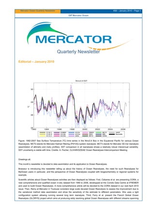
  • 1. Mercator Ocean Quarterly Newsletter #36 – January 2010 – Page 1 GIP Mercator Ocean Quarterly Newsletter Editorial – January 2010 Figure: 1992-2007 Sea Surface Temperature (ºC) time series in the Nino3.4 Box in the Equatorial Pacific for various Ocean Reanalyses. MCT2 stands for Mercator Kalman filtering (PSY2G) system reanalysis. MCT3 stands for Mercator 3D-Var reanalysis (assimilation of altimetry and insitu profiles). SST comparison in all reanalyses shows a relatively robust interannual variability. SST uncertainty is stable with time. Credits: A. Fischer, CLIVAR/GODAE Ocean Reanalyses Intercomparison Meeting. Greetings all, This month’s newsletter is devoted to data assimilation and its application to Ocean Reanalyses. Brasseur is introducing this newsletter telling us about the history of Ocean Reanalyses, the need for such Reanalyses for MyOcean users in particular, and the perspective of Ocean Reanalyses coupled with biogeochemistry or regional systems for example. Scientific articles about Ocean Reanalyses activities are then displayed as follows: First, Cabanes et al. are presenting CORA, a new comprehensive and qualified ocean in-situ dataset from 1990 to 2008, developped at the Coriolis Data Centre at IFREMER and used to build Ocean Reanalyses. A more comprehensive article will be devoted to the CORA dataset in our next April 2010 issue. Then, Remy at Mercator in Toulouse considers large scale decadal Ocean Reanalysis to assess the improvement due to the variational method data assimilation and show the sensitivity of the estimate to different parameters. She uses a light configuration system allowing running several long term reanalysis. Third, Ferry et al. present the French Global Ocean Reanalysis (GLORYS) project which aims at producing eddy resolving global Ocean Reanalyses with different streams spanning
  • 2. Mercator Ocean Quarterly Newsletter #36 – January 2010 – Page 2 GIP Mercator Ocean different time periods and using different technical choices. This is a collaboration between Mercator and French research laboratories, and is a contribution to the European MyOcean project. Then, Masina et al. at CMCC in Italy are presenting the implementation of data assimilation techniques into global ocean circulation model in order to investigate the role of the ocean on climate variability and predictability. Fifth, Smith et al. are presenting the Ocean Reanalyses studies at ESSC in the U.K. which aim at reconstructing water masses variability and ocean transports. Finally, Langlais et al. are giving an example of the various uses of ocean reanalyses: they are using the Australian BlueLink Reanalysis in order to look into details at the various Southern Ocean fronts. The next April 2010 newsletter will introduce a new editorial line with a common newsletter between the Mercator Ocean Forecasting Center in Toulouse and the Coriolis Data Center at Ifremer in Brest. Some papers will be dedicated to observations only, when others will display collaborations between the 2 aspects: Observations and Model. The idea is to wider and complete the subjects treated in our newsletter, as well as to trigger interactions between observations and modeling communities. This common Mercator-Coriolis Newsletter is a test for which we will take the opportunity to ask for your feedback. We wish you a pleasant reading!
  • 3. Mercator Ocean Quarterly Newsletter #36 – January 2010 – Page 3 GIP Mercator Ocean Contents Ocean reanalyses: prospects for multi-scale ocean variability studies .............................................................4 By Pierre Brasseur CORA -Coriolis Ocean database for Re-Analyses-, a new comprehensive and qualified ocean in-situ dataset from 1990 to 2008............................................................................................................................................5 By Cécile Cabanes, Clément de Boyer Montégut, Karina Von Schuckmann, Christine Coatanoan, Cécile Pertuisot, Loic Petit de la Villeon, Thierry Carval, Sylvie Pouliquen and Pierre-Yves Le Traon Large scale ocean variability estimated from a 3D-Var Reanalysis: sensitivity experiments.............................8 By Elisabeth Remy Mercator Global Eddy Permitting Ocean Reanalysis GLORYS1V1: Description and Results ............................ 15 By Nicolas Ferry, Laurent Parent, Gilles Garric, Bernard Barnier, Nicolas C. Jourdain and the Mercator Ocean team Re-analyses in the Global Ocean at CMCC-INGV: Examples and Applications................................................. 28 By Simona Masina, Pierluigi Di Pietro, Andrea Storto, Srdjan Dobricic, Andrea Alessandri, Annalisa Cherchi Ocean Reanalysis Studies in Reading: Reconstructing Water Mass Variability and Transports....................... 39 By Gregory C. Smith, Dan Bretherton, Alastair Gemmell, Keith Haines, Ruth Mugford, Vladimir Stepanov , Maria Valdivieso and Hao Zuo Southern Ocean Fronts in the Bluelink Reanalysis.......................................................................................... 50 By Clothilde Langlais, Andreas Schiller and Peter R. Oke Notebook....................................................................................................................................................... 58
  • 4. Mercator Ocean Quarterly Newsletter #36 – January 2010 – Page 4 Newsfeature Ocean reanalyses: prospects for multi-scale ocean variability studies By Pierre Brasseur MEOM-LEGI, Grenoble France Over the past decade, the ocean weather prediction community has made terrific progress toward the establishment of an effective infrastructure for systematic acquisition and processing of in situ and space observations, assimilation of data into global, high-resolution ocean circulation models for real-time nowcast and short-range forecast, and delivery of synthetic products to users. This Operational Oceanography infrastructure represents a unique opportunity for applications that require time series describing the evolution of ocean state over sufficiently long periods of time (~ 20 to 50 years) to have value for climate research as well as for regional studies of the ocean variability. The vast majority of ocean weather prediction systems in operation indeed have the capacity to resolve the whole spectrum of interacting scales from mesoscale eddies to planetary waves, and this is believed to be a key asset for investigating climate-related modes of the ocean variability. The application of an ocean weather prediction system to this purpose, however, is neither trivial nor immediate. Structural changes (e.g. in model resolution, data provision, or assimilation schemes) implemented intermittently in operational suites affect the accuracy of analyses and make the sequence of estimated ocean states inhomogeneous in quality. As a result, series of 3-D ocean analyses produced in real-time for nowcast purposes cannot be used for consistent exploration of ocean variability aspects such as trends and low-frequency signals. Instead, better products can be generated retrospectively by re-analysing past observations with a fixed ocean model and a fixed data assimilation scheme in which the best available parameterizations and assimilation options have been prescribed. A retrospective analysis, or reanalysis, offers the possibility of extracting additional information from data sets generated a posteriori with improved reprocessing algorithms. Reanalyses can therefore contribute to more confident attribution of the processes that are responsible for the observed variability as well as the expected geographical patterns and magnitudes of the responses. In return, reanalysis products could ultimately provide relevant information on how to design appropriate observing systems and optimized sampling strategies for the ocean, especially for the detection of climate variability signals. Dedicated Observation Sensitivity Experiments (OSEs) for instance, can provide information about the sensitivity of reanalyses to the density of the observation network. In essence, the systems that are producing 4-D historical reconstructions should be different from those used in real-time. An obvious difference when operating an assimilation system in retrospective mode lies in the possibility of using both “past” and “future” observations. This motivates the development of new assimilation algorithms, such as Kalman-type smoothers that, in the future, should supersede the Kalman-type filters currently available in most operational centers. Another fundamental difference between a reanalysis and a raw sequence of ocean state estimations produced at discrete time intervals lies in the “dynamical” dimension, which should be very carefully taken into account for the reconstruction of 4-D fields. The dynamical constraints imposed by physical laws are critical for inferring unobserved quantities such as currents, or to compute transport of tracers and integrated circulations through sections. To some extent however, the requirement for dynamical consistency over periods of time larger than the predictability time scales of the simulated flow remains an issue at conceptual level. This is especially true with eddy-resolving ocean models for which the so-called “weak-constraint” assimilation methods (i.e. assuming that the model equations are not strictly verified) represent the relevant framework to properly conciliate imperfect models with imperfect data. Other key challenges will have to be addressed in the future, such as reanalyses with coupled components of the ocean- atmosphere-biosphere system and the need for consistent uncertainty estimates on the solutions. Ensemble methods are already being implemented for nowcast and short–term predictions, and provide an elegant and powerful statistical methodology to quantify uncertainty. However, running ensembles of statistical significance still represent a major computational issue with regard to the production of multi-decadal data sets. The same difficulty exists for variational assimilation methods, as in this case the error estimation process requires the computation of the inverse of the Hessian of the cost function. The reanalysis concept has been proven first in the atmosphere in the eighties, and atmospheric reanalyses have become an essential by-product of major numerical weather prediction systems. In oceanography, reanalyses of the global ocean/sea-ice system have already been produced under the auspices of GODAE and CLIVAR, leading to intercomparison exercises coordinated at international level. Today, the production and delivery of ocean reanalyses is identified as a major task for the future Marine Core Services of GMES. In the framework of the EU-funded MyOcean project, several monitoring and forecasting centers (Mercator, INGV, MetNo …) are committed to provide qualified reanalyses to users from different applicative sectors (climate, seasonal and weather forecasting, management of marine resources, coastal environment monitoring and assessment). No doubt that users will be increasingly demanding in terms of quality and validation of products, and this will represent a very significant driver for the whole Operational Oceanography community in the next decade.
  • 5. Mercator Ocean Quarterly Newsletter #36 – January 2010 – Page 5 CORA -Coriolis Ocean database for Re-Analyses-, a new comprehensive and qualified ocean in-situ dataset from 1990 to 2008 CORA -Coriolis Ocean database for Re-Analyses-, a new comprehensive and qualified ocean in-situ dataset from 1990 to 2008 By Cécile Cabanes 1 , Clément de Boyer Montégut 1 , Karina Von Schuckmann 1 , Christine Coatanoan 2 , Cécile Pertuisot 2 , Loic Petit de la Villeon 2 , Thierry Carval 2 , Sylvie Pouliquen 1 and Pierre-Yves Le Traon 1 1 Laboratory of Oceanography from Space (LOS), IFREMER/CNRS, Brest, France 2 Coriolis Data Centre, IFREMER, Brest, France Introduction An ideal set of oceanographic data would comprehends a global coverage, continuity in time, is subject to regular quality controls and calibration processes (i.e. durable in time), and encompasses several space/time scales. This goal is actually not easy to reach and reality is often different especially with in-situ oceanographic data, such as temperature and salinity profiles in our case. Those data have basically as many origins as there are scientific campaigns to collect them. Some efforts to make such an ideal dataset have been done for many years, especially since the initiative of Levitus (1982). A program named Coriolis has been set up at Ifremer data centre the beginning of the 2000's in the wake of the development of operational oceanography in France. The project was launched in order to contribute to the ocean in situ measurements part of the French operational system (e.g. Mercator group). It has been especially involved in developing continuous, automatic, and permanent observation networks. The data centre is gathering ocean data in real time, which are then subject to its own quality procedures (Coatanoan and Petit de la Villéon, 2005). Our goal now is to distribute an extraction of this comprehensive and reprocessed set of ocean in-situ data, from 1990 to 2008. The aim is to publish this qualified dataset for operational as well as for research purposes. In doing this work, we can also evaluate the difference between our dataset and state of the art databases like the World Ocean Database 2009 (Boyer et al, 2009) for example. This is also a way to improve the quality of this “living” real time database. We first present a description of the dataset and of the quality controls applied, then we give examples of the main uses for which those data are meant for. Description of the Dataset Overview The CORA dataset basically contains global, sub-surface ocean profiles of in-situ temperature and salinity at observed levels. Those data were extracted from the real-time CORIOLIS database at the beginning of 2008 (and early 2009 for 2008 data). From those raw data, we construct and make available profiles data at standardized levels, and gridded fields of T/S obtained through objective analysis. Data type CORA contains data from different types of instruments: mainly Argo floats, XBT, CTD and XCTD, and Mooring Data (see figure 1). The Coriolis centre receives data from Argo program, French research ships, GTS data, GTSPP, GOSUD, MEDS, voluntary observing and merchants ships, moorings, and the World Ocean Database (not in real time for the last one). Quality controls To produce this dataset, several tests have been developed in order to improve the quality flags of the raw database and to fit the level required by the physical ocean re-analysis activities. These tests include some simple systematic tests, a test against climatology and a more elaborate statistical test involving an objective analysis method (see Gaillard et al., 2009 for further details). Visual quality control (QC) is performed on all the suspicious temperature (T) and salinity (S) profiles. The statistical test is based on an objective analysis run with a three weeks window in order to capture the most doubtful profiles. They are then visually checked by an operator who decides whether or not they are bad data or real oceanic phenomena. Then a second run which takes into account only the good data is operated on a one week window in order to produce the gridded fields. Each release provides T and S gridded fields and individual profiles both on their original levels and interpolated levels.
  • 6. Mercator Ocean Quarterly Newsletter #36 – January 2010 – Page 6 CORA -Coriolis Ocean database for Re-Analyse-, a new comprehensive and qualified ocean in-situ dataset from 1990 to 2008 Figure 1 Temporal (left) and spatial distribution in 2007 (right) for the different type of data used in CORA. Goals and uses of the Dataset Research CORA database is meant to investigate specific scientific questions. Achieving this goal will lead to the improvement of the quality of the dataset, by detecting abnormal data especially. That will benefit subsequently to the data centre real-time database and the operational results. It is also a way to monitor ocean variability as it is done on the framework of the MyOcean European project (http://www.myocean.eu.org/). This dataset can be used to estimate the change in global ocean temperature and heat content during the 2003-2008 time period. As shown in previous results, the world ocean is warming (e.g. Levitus et al., 2005). The work of von Schukmann et al. (2009) shows that the signal propagates to increasing depth in time, especially in the northern hemisphere. The average warming rate is 0.77 ± 0.11 W/m2 for the 0-2000m depth layer during 2003-2008. Ocean model validations CORA can be used to construct elaborated products such as climatologies of heat content, depth of the thermocline or 20°C isotherms, or indexes (niño3.4, MOC, PDO…). Such products are especially useful for validating ocean model outputs and improve their quality or assess their results. For example, de Boyer Montégut et al. (2007) validates their OGCM mixed layer depth outputs against in-situ observations in the northern Indian Ocean. After assessing the realism of their experience, they use the model to investigate surface heat budget variability. Assimilation in ocean models An important application of such a database is also for ocean model assimilation projects. In France, the goal of GLORYS (GLobal Ocean ReanalYsis and Simulations) project is to produce a series of realistic eddy resolving global ocean reanalyses. Several reanalyses are planned, with different streams. Each stream can be produced several times with different technical and scientific choices. Version 1 of Stream 1 (GLORYS1V1) is produced using the previous version of the CORA data set (see Ferry et al, this issue) and is available on request from products@mercator-ocean.fr. The ocean general circulation model used is based on ORCA025 NEMO OGCM configuration (Barnier et al., 2006).
  • 7. Mercator Ocean Quarterly Newsletter #36 – January 2010 – Page 7 CORA -Coriolis Ocean database for Re-Analyse-, a new comprehensive and qualified ocean in-situ dataset from 1990 to 2008 Références Barnier B., G. Madec, T. Penduff, J.-M. Molines, A.-M. Treguier, J. Le Sommer, A. Beckmann, A. Biastoch, C. Böning, J. Dengg, C. Derval, E. Durand, S. Gulev, E. Remy, C. Talandier, S. Theetten, M. Maltrud, J. McClean and B. De Cuevas et al., 2006: Impact of partial steps and momentum advection schemes in a global ocean circulation model at eddy permitting resolution. Ocean Dynamics, DOI: 10.1007/s10236-006-0082-1. Boyer T.P., J. I. Antonov, O. K. Baranova, H. E. Garcia, D. R. Johnson, R. A. Locarnini, A. V. Mishonov, D. Seidov, I. V. Smolyar, and M. M. Zweng, 2009: World Ocean Database 2009, Chapter 1: Introduction, NOAA Atlas NESDIS 66, Ed. S. Levitus, U.S. Gov. Printing Office, Wash., D.C. , 216 pp., DVD. de Boyer Montégut, C., J. Vialard, S. S. C. Shenoi, D. Shankar, F. Durand, C. Ethé, and G. Madec, 2007,:Simulated seasonal and interannual variability of mixed layer heat budget in the northern Indian Ocean, J. Climate, 20, 3249-3268 Coatanoan C., and L. Petit de la Villéon, 2005: Coriolis Data Centre, In-situ data quality control procedures, Ifremer report, 17 pp. (http://www.coriolis.eu.org/cdc/quality_control.htm) Gaillard F., E. Autret, V. Thierry, P. Galaup, C. Coatanoan, and T. Loubrieu, 2009: Quality controls of largeArgo datasets, J. Atmos. Ocean. Tech., 26, 337-351 Levitus, S., 1982: Climatological Atlas of the World Ocean, NOAA Professional Paper 13, U.S. Government Printing Office, Rockville, M.D., 190 pp. Levitus, S., J. Antonov, and T. Boyer, 2005: Warming of the world ocean, 1955-2003, Geophys. Res. Lett., 32. von Schukmann, K., F. Gaillard and P.Y. Le Traon, 2009: Global hydrographic variability patterns during 2003-2008, J. Geophys. Res.
  • 8. Mercator Ocean Quarterly Newsletter #36 – January 2010 – Page 8 Large scale ocean variability estimated from a 3D-Var Reanalysis at Mercator: sensitivity experiments Large Scale Ocean Variability Estimated from a 3D-Var Reanalysis at Mercator: Sensitivity Experiments By Elisabeth Remy 1,2 1 CERFACS, Toulouse, France 2 MERCATOR-OCEAN, Toulouse, France Introduction Ocean reanalysis aims at combining available observations with a general circulation model (GCM) to provide a more accurate description of the historical ocean state than can be obtained by model or observations alone. In this context, the model can be interpreted as a space-time dynamical interpolator of the observations. Here we consider a large scale decadal ocean reanalysis that has been produced by combining in situ and altimeter observations with a global ocean GCM using a three-dimensional variational (3D-Var) approach. Our objective is to assess the improvement brought by data assimilation and to illustrate the sensitivity of the ocean state estimates to different assimilation configurations. We focus on the large scale interannual variability. Model configuration The ocean model is the LOCEAN primitive equation model OPA8.2 (Madec et al., 1998) in its low resolution configuration ORCA2°. The version of the model used here is a fre e-surface constant volume configuration. Atmospheric forcing fields are applied as “forced flux”. They are derived from the ECMWF atmospheric reanalysis ERA40. After year 2001 when ERA40 is not available, they are taken from ECMWF operational analyses. A strong restoring term to the weekly Reynolds SST is applied, with a coefficient of 200W/m2. The ERA precipitation field has been bias corrected using GPCP precipitation data (Troccoli and Källberg, 2004). As the global water mass budget is not closed due to large errors in the fresh water fluxes, an additional constraint is applied to close the budget. As a consequence, the model is unable to represent that part of the eustatic trend due to atmospheric mass input observed in altimeter observations. Variational assimilation method / code The assimilation system is based on the OPAVAR system developed at CERFACS. The model configuration and assimilation parameters are very close to the setup of the ENSEMBLE experiments. A detailed description of the assimilation system and reanalysis procedure can be found in Daget et al. (2009). The major difference with our system is that we assimilate along track Sea Level Anomalies. Here we quickly recall the basis of the variational approach. The 4dvar method is based on minimization of a cost function which contains the square root of the observation misfits and a priori information on the solution. The minimum, x*, is a model trajectory close to the observations in agreement with the prescribed model and observation errors. The problem to solve can be expressed as follows: x* as J(x*)=min(J(x)), (eq. 1) x verifying the model equation : xi+1=M(xi) where : J(x) = ½ [x0-x0 b ] T B-1 [x0-xb0 b ] + ½ Σ[H(xi) – yo ]T R-1 [H(xi) – yo ] (eq. 2) Here we search the optimal initial conditions, x0. - x0 is the control vector we want to estimate: it contains the uncorrelated model state variable, x0 b is the background estimate, usually taken as the final state of the previous assimilation cycle, - B is the background model error covariance matrix, - yo observation vector, - R is the observation error covariance matrix This minimization of the cost function is done iteratively using a descent algorithm: at each iteration the gradient is used to compute a new correction in the direction of the minimum. This allows taking into account the non linearity of the model equations.
  • 9. Mercator Ocean Quarterly Newsletter #36 – January 2010 – Page 9 Large scale ocean variability estimated from a 3D-Var Reanalysis at Mercator: sensitivity experiments The 3dvar FGAT (First Guess at Appropriate Time) is derived from the incremental formulation of the 4Dvar. In the 3dVar FGAT approximation, the cost function is linearized and the gradient to compute the descent direction is approximated. The innovation, yo-H(xib), is computed at the observation time. The method is described in Weaver et al. (2003,2005). The assimilation window for the experiment presented here is 10 days. The background error covariance matrix, B, contains the variance of the model error on the diagonal, covariance terms and spatial correlation specification off diagonal. The standard deviation prescribed for each control variable depends on the current state of the ocean. The multivariate relations link the model variables using dynamical or physical relationships between the variables. For example, the “salinity balance operator” (Ricci et al, 2005) preserves the water mass properties, insuring that salinity varies according to temperature changes, even without any salinity data assimilated. First order physical equilibrium are also prescribed between the other variables, as the geostrophic equilibrium for velocity, steric component for the sea level. Observations Before assimilating observations, it is important to understand their information content, the data processing, and possible filtering, subsampling, in order to precisely compute their equivalent with the model variables and the error estimate. In situ profiles : observation data sets For the experiments described here we used the quality-controlled ENSEMBLES (EN3 v1a) in situ dataset produced at the Met Office. Details on the databases used to construct it and the quality control checks that were applied can be found on the dedicated webpage (http://hadobs.metoffice.com/en3/) and in the article by Ingleby and Huddleston (2007). Sea level anomaly data The dynamic topography reflects the elevation of sea level due to ocean currents, the steric expansion of the water, and mass forcing from land and atmosphere. It can be defined as the sum of a time mean, the so called Mean Dynamic Topography (MDT) and time variations about this mean: Sea Level Anomalies (SLA). Satellite altimeters estimate the distance to the sea surface, providing accurately the variations of the sea surface. Important pre-treatment of the data are done in order to correct this distance from propagation error in the atmosphere, tides, etc... Along track SLA are assimilated. A delayed time product from AVISO is chosen due to a higher quality of the post processing and its homogeneity over the time period. The observation error covariance matrix, R, is diagonal. It represents the confidence interval given to the observation compared to its model equivalent. It takes into account not only the measurement error but also the representativity error. The measurement error can contain an instrument error and treatment error, as the representivity error contains signals viewed by observations but not represented by the model. This part of the error can be dominant especially with low spatial resolution model like ORCA2. The model is not able to represent explicitly the mesoscale activity, sharp fronts, etc… The estimation of the representativity error is based on the statistical approach (Fu et al, 1993) under the hypothesis of uncorrelated observation error. The underlying assumption is that the representativity error can be computed using the variance of the observations compared to the variance of the model. Figure 1 shows the representativity error estimated for the in situ temperature observations and along track sea level anomalies. Figure 1 Representativity error maps for temperature observations (longitudinal mean for the global ocean) in °C and along track sea level anomalies in mm.
  • 10. Mercator Ocean Quarterly Newsletter #36 – January 2010 – Page 10 Large scale ocean variability estimated from a 3D-Var Reanalysis at Mercator: sensitivity experiments Experiment setup We define a default experiment covering the period 1960-2005 using the available observations, in situ and SLA referenced to the model MDT. The model counter part of the observations is computed at the nearest time step. For moored buoy data (e.g., TAO), the model equivalent is a daily mean model temperature field. In space, the model counterpart is computed with an interpolation from the model grid to the observation point. Different experiments were also done to test the sensitivity of the estimated ocean circulation to the MDT and the type of assimilated observations. The table 1 summarizes the setup of those experiments. Time frame In situ observations SLA observations Control 1960-2005 No No b090 1960-1992 Yes No b09a 1993-2005 Yes No b09b 1993-2005 Yes Yes + Model MDT b09c 1993-2005 Yes Yes + Rio MDT Table 1 Experiments setup To follow the global sea level rise observed from altimetry measurements, we let the global mean sea level in the model adjust freely. Note that theoretically, the correct approach would be to remove from the SLA observations this signal that the model is not able to properly represent: the global mass budget is forced to zero in the model and the model is built with a volume conservation hypothesis. Sensitivity experiments The sensitivity of the linear trend of different diagnosed quantities is presented here. We focus on the period 1993-2001 where we compare the trends estimated from the model with the trend estimated from observations. In experiment b09a only in situ observations are assimilated, while in b09b and b09c, SLA observations are assimilated in addition. The MDT used in the b09b experiment is the model MDT computed from the control model simulation whereas in b09c it is the Rio MDT (Rio and Hernandez, 2004) (Table 1). Estimates of the 0-300 meter mean temperature, salinity and sea level linear trends are presented in Figure 2. We compare the temperature estimation to monthly objectively analyzed subsurface temperature by Ishii et al.(2003) The analysis is based on different datasets including the World Ocean Database/Atlas. Globally, one can see very similar estimates of the mean temperature trend over the first 300 meters in the different assimilation experiments, comparable to the observed trend. This robustness can be attributed to the data density which allows controlling this variable. In the Southern ocean were data are very sparse, solutions slightly differ. The observations analysis, done by Ishii et al. (2003), does not show significant trend in this region. The salinity trend appears to be extremely sensitive and strongly differs between experiments. Unrealistically strong trends appear in the southern hemisphere when altimeter data are assimilated. The trend is even stronger when the Rio MDT is used. The sea level trend is already well constrained by the in situ observations. The assimilation of altimeter data improves the amplitude. The trend is then very close to the observed one for whichever MDT is chosen. To understand these results, we note that both in situ and SLA observations contain information on the temperature and salinity field. The in situ data provide direct information through T and S profiles, whereas the sea level data (MDT+SLA) reflect the heat and haline content over the whole water column due to the sea water expansion. A hypothesis is that the salinity tends to compensate the inconsistency between the dynamic height deduced from the MDT+SLA and from the in situ observations due to the use of different MDTs compared to the real one. The northern hemisphere is less sensitive probably due to a larger amount of salinity data in this region. For all these diagnostics, the simulation without assimilation shows the right large scale patterns but with unrealistically small amplitudes: the impact of the assimilation is clearly positive in this respect.
  • 11. Mercator Ocean Quarterly Newsletter #36 – January 2010 – Page 11 Large scale ocean variability estimated from a 3D-Var Reanalysis at Mercator: sensitivity experiments 0-300 m temperature trend (°C) 0-300 salinity trend (PSU) Sea Level trend (m) controlrunInsitu(b09a)Insitu;SLA+model MDT(b09b)MDT Insitu;SLA+RioMDT (b09c) Observationanalysis Ishii analysis AVISO maps Figure 2 1993-2001 0-300 m temperature (°C), salinity (PSU) and sea level (m) linear trend from assimilation experiments and from analysis of observations Analysis of the reference simulation 1960-2005 We illustrate the reanalysis results with a few diagnostics focusing on the subsurface representation of the ocean interannual variability estimated from the experiments b090 and b09b over the period 1960-2005 (Table 1). The large increase of the number of in situ observations at the beginning of the ARGO era improves the control of the ocean model variables: the mean misfit to the in situ observations is significantly reduced from 1960 to 2005, especially between 300 and 700 meters depth (not shown here). Temperature, salinity and SSH trend The temperature linear trend from 1960 to 2005 is clearly non uniform (Figure 3, left panel). The North Atlantic is warming, as the Pacific is cooling in the subtropical gyre and warming in the southern part. The vertical mean profile temperature evolution for the North East Atlantic (box shown on the temperature trend map) is presented on the right. Mode water formation occurs in this
  • 12. Mercator Ocean Quarterly Newsletter #36 – January 2010 – Page 12 Large scale ocean variability estimated from a 3D-Var Reanalysis at Mercator: sensitivity experiments region of subduction. Successive warm and cold signals propagate from the surface to deeper layers. This clearly shows the importance of the long term variability in the ocean. The situation is very different depending on the region we look at. Figure 3 Mean 0-300 m temperature trend 1960-2005 on the left and mean temperature vertical profile evolution in the north east Atlantic (box on the left map) on the right, in °C. Figure 4 represents the estimated linear trend of the sea level rise on the left and the dynamic height on the right. The Atlantic Ocean shows a rising sea level in the middle of the subtropical gyres, whereas the Pacific Ocean shows different tendencies depending on the latitude. The dynamical height reflects the steric part of the sea level. The differences with the sea level are due to mass changes: advection or input from land, including ice cap or atmosphere. They appear mainly in the southern Pacific Ocean and the Indian Ocean. The partition of the SLA into an eustatic and a steric contribution (dynamic height) is sensitive to the specification of the background error covariance between the different model variables in B (eq. 2). The full model description of the ocean state allows us to decompose the dynamic height into its thermosteric and halosteric part. Those components (not shown here) have opposite contributions: the halosteric tends to moderate the thermosteric part which has an even higher trend than the total dynamical height. Figure 4 Sea level (left) and dynamical height (right) linear trend from 1960 to 2005 in meters. Interannual variability Up to now we have looked at the linear trend, while here we illustrate the use of the reanalysis to examine the interannual variability. A projection on Empirical Orthogonal Functions (EOF) gives an interesting way to analyse the variability of the ocean circulation. The modest size of the model state vector in ORCA2 allows us to perform this computation easily on the 45 years of the simulation. Figure 5 shows the different spatial patterns associated with the first 3 EOFs of the mean temperature over 0-300m. The EOF coefficient time series is also presented. The seasonal signal has been removed. The ENSO pattern is largely dominant and corresponds to the 1st EOF which explains 26% of the variance. The balance between the eastern and western part represents the change of the slope of the thermocline. The link with the Indian Ocean also clearly appears. The signal in the Atlantic is too small to be significant. The second EOF is also mainly related to tropical Pacific dynamics, while in the Atlantic Ocean a quasi- uniform pattern exists. The third EOF looks like the warming trend, especially in the Atlantic Ocean. The fourth panel of Figure 5
  • 13. Mercator Ocean Quarterly Newsletter #36 – January 2010 – Page 13 Large scale ocean variability estimated from a 3D-Var Reanalysis at Mercator: sensitivity experiments shows the time evolution of the coefficients of the 1st three EOFs. The red curve corresponds to the first EOF, the green one to the second EOF, and the blue one to the third EOF. Figure 5 First three EOFS of the decomposition of the mean 0-300m temperature and the time series of the coefficients from 1960 to 2005 (1st eof in red, second in green, third in blue). Conclusion This study shows that even with a low resolution ocean model, the large scale variability of the upper ocean can be effectively constrained by assimilating in situ profiles and sea level observations. Some estimates are robust and close to the observed one; others appear to be more sensitive, like salinity. The low resolution configuration provides a useful tool for sensitivity experiments which are too expensive with high resolution models. The comparison of the reanalysis results with the forced run without assimilation shows a significant improvement in the amplitude of the variability of the upper ocean temperature field. The MERCATOR Glorys reanalysis is based on the ORCA ¼° global configuration and the SAM2 assimilation scheme using local inversions. It will be interesting to test the control of the large scale with this 3D-Var complementary to the local analysis method. Acknowledgements I would like to thank Anthony Weaver for his comments on this article. References Fu L.L., I. Fukumori, and R.N. Miller, 1993: Fitting dynamic models to the geosat sea level observations in the tropical Pacific Ocean. part ii : A linear, wind-driven model. Journal of Physical Oceanography, 23, p. 2162-2181. Ingleby, B., and M. Huddleston, 2007: Quality control of ocean temperature and salinity profiles - historical and real-time data. Journal of Marine Systems, 65, 158-175. Ishii, M., M. Kimoto, M. Kachi, 2003: Historical Ocean Subsurface Temperature Analysis with Error Estimates, Monthly Weather Review, Vol. 131, Issue 1, p. 51-73. Madec, G., P. Delecluse, M. Imbard and C. Levy, 1998: OPA 8.1 Ocean General Circulation Model reference manual. Tech. rep., Institut. Pierre-Simon Laplace (IPSL), France, No11, 91pp. Ricci S., A. T. Weaver, J. Vialard, P. Rogel, 2005: Incorporating State-Dependent Temperature–Salinity Constraints in the Background Error Covariance of Variational Ocean Data Assimilation, Monthly Weather Review, Vol. 133, Issue 1, p. 317-338.
  • 14. Mercator Ocean Quarterly Newsletter #36 – January 2010 – Page 14 Large scale ocean variability estimated from a 3D-Var Reanalysis at Mercator: sensitivity experiments Rio, M.-H., and F. Hernandez, 2004: A mean dynamic topography computed over the world ocean from altimetry, in situ measurements, and a geoid model, J. Geophys. Res., 109, C12032. Weaver A. T, J Vialard, and D. L. T Anderson, 2003: Three- and four-dimensional variational assimilation with a general circulation model of the tropical Pacific Ocean. Part I: Formulation, internal diagnostics, and consistency checks. Mon. Wea. Rev., 131, 1360–1378.
  • 15. Mercator Ocean Quarterly Newsletter #36 – January 2010 – Page 15 Mercator Global Eddy Permitting Ocean Reanalysis GLORYS1V1 : Description and Results Mercator Global Eddy Permitting Ocean Reanalysis GLORYS1V1: Description and Results By Nicolas Ferry1 , Laurent Parent1 , Gilles Garric1 , Bernard Barnier2 , Nicolas C. Jourdain2 and the Mercator Ocean team. 1 Mercator Océan, Ramonville St Agne, France 2 MEOM-LEGI, CNRS, Université de Grenoble, Grenoble, France Abstract We present here preliminary results from the French Global Ocean Reanalysis and Simulations (GLORYS) project which aims at producing a series of global ocean reanalyses. This project is a collaboration between Mercator-Ocean and French research laboratories, and is a contribution to the project of the European Union MyOcean. The overall objective is to produce state of the art eddy resolving global ocean simulations constrained by oceanic observations by means of data assimilation. GLORYS plans to produce different streams, spanning different time periods and using different technical choices. Here, we present GLORYS1V1 (the first version of the stream 1 reanalysis) covering the “Argo” era (2002-2008), a period characterized by its unique high density of remotely sensed and in situ observations. Assimilation diagnostics as well as the evaluation of the representation of some circulation features are presented. Introduction In the last decade, real-time high-resolution ocean analysis and forecasting have become routine tasks done by several operational centers throughout the world (Dombrowsky et al. 2009). Downstream applications of these near real-time operational analyses and forecasts have been demonstrated in many areas such as marine pollution monitoring (Hackett et al. 2009) and marine safety (Davidson et al. 2009), coastal modelling (De Mey et al. 2009), ocean initialization for seasonal forecasting (Balmaseda et al. 2009), support to the navies (Jacobs et al. 2009), biochemistry modeling (Brasseur et al. 2009) etc. Some specific applications of ocean state estimation however require long time series of the three dimensional ocean state called ocean reanalyses. Several groups have produced in the last years ocean reanalyses spanning, for the longest one, the 1960-present time period (Lee et al. 2009). This kind of product is used mostly for climate research, (Lee at al. 2009), for long coupled ocean- atmosphere hindcasts for seasonal forecasts (Balmaseda et al. 2009), and helps to the building of new climate indicators for coastal upwelling, precipitation and extreme weather events such as tropical storms and cyclones (Xue et al. 2009). Most of the ocean reanalyses are available at coarse resolution (Rienecker et al. 2009) with a horizontal resolution of ~1°and do not include explicitly the mesoscale effects in the estimation of the ocean state. This means that during the altimetric years (1992- present) the observed eddy variability and its subsequent effects (e.g. eddy induced transports) may not be properly taken into account. Another reason why higher resolution reanalyses should be carried out is that fronts (associated to western boundary currents for example) are better resolved and regional biases (like the Gulf Stream overshoot) are reduced. Lastly, high resolution reanalyses should also be beneficial for downstream applications of like biogeochemical modelling or regional / coastal modelling. With its experience in the field of ocean analysis and forecasting, Mercator has developed a global ocean eddy permitting resolution (1/4°) reanalysis system. This work is d one in the framework of the French GLobal Ocean ReanalYsis and Simulations (GLORYS) and the EU funded MyOcean projects. The objective is to produce a series of realistic (i.e. close to the existing observations and consistent with the physical ocean) eddy resolving global ocean reanalyses. Here we present the stream 1 reanalysis (called GLORYS1V1) spanning the 2002-2008 time period (the “Argo” era). The reanalysis system is similar in many aspects to the Mercator operational ¼° global ocean analysis/prediction system (Dombrowsky et al. 2009). However, GLORYS1V1 benefits from significant improvements that are presented here. This paper describes the way Mercator operational ¼°global ocean analysis / forecast system has been modified to produce a 7-year reanalysis. Then, the results of the reanalysis are presented and compared to the operational system in 2007-2008. Description of GLORYS1V1 reanalysis system The ocean reanalysis system used (called GLORYS1V1) is based on the operational system PSY3V2 used at Mercator1. GLORYS1V1 benefits from several improvements that we present in the following section. We describe the different components, namely the ocean/sea-ice model, the data assimilation method, the ocean initialization and the observations assimilated. We also 1 (http://bulletin.mercator-ocean.fr/html/produits/psy3v2/psy3v2_courant_en.jsp)
  • 16. Mercator Ocean Quarterly Newsletter #36 – January 2010 – Page 16 Mercator Global Permitting Ocean Reanalysis GLORYS1V1 : Description and Results carefully review the improvements with respect to the operational system. Table 1 summarizes the main differences between the operational system PSY3V2 and GLORYS1V1. The starting date of GLORYS1V1 simulation is 3 October 2001. Ocean-sea ice model The model configuration is the same as the one used in the operational global ocean system operated in near real time at Mercator since November 2005 (Drevillon et al. 2008a, Drevillon et al. 2008b). It is a global implementation of the ocean/sea-ice NEMO numerical framework (version 1.09, Madec, 2008) and has many common features with the ORCA025 configuration developed by the European DRAKKAR collaboration (Drakkar group, 2007), the numerical details of which are given in Barnier et al. (2006). The ocean model component is the free surface, primitive equation ocean general circulation model developed at LOCEAN (Madec, 2008). The sea-ice component is the LIM2 sea-ice model (Goosse and Fichefet, 1999). The geographical domain extends from -77°S to the North Pole. The ve rtical discretisation uses partial steps with 50 vertical levels with an increased resolution near the surface (~1 m near the surface, 11 levels over the top 15m, 500 m at depth). Compared to the operational system PSY3V2, the sea-ice model used for GLORYS1V1 benefits from the following improvements: (i) an Elastic Viscous Plastic (EVP) dynamics of the ice and (ii) a computation at each time step of the ocean-ice stress. These two new parameterizations improve clearly the results of the ice model, in particular the ice extent during summer in the Arctic Ocean (Garric et al., 2008). This improved ice model version is referred to as LIM2_EVP. The CLIO bulk formula (Goose et al., 2001) are used in both GLORYS1V1 and the operational system to calculate the atmospheric forcing function. They are fed with surface variables from ECMWF operational analyses (1-day averages). The ECMWF precipitation field is corrected using GPCP monthly data (Garric, 2006) in a way similar to that proposed by Troccoli and Källberg (2004). This correction is however not sufficient to constrain the global average water budget (evaporation, precipitation and runoff) to a realistic value. That is why the global water budget is set to zero at each time step. Initial conditions used for the ocean are derived from the ARIVO climatology (Gaillard et al. 2008, Gaillard and Charraudeau, 2008) for the month of October. The sea ice initial condition is the sea ice state in October 2001 from a multi decadal model integration performed by the DRAKKAR group (namely G70, Drakkar Group 2007) with the same ocean-sea-ice model. Data assimilation method The data assimilation method developed at Mercator (Tranchant et al. 2008) is used in GLORYS1V1. The assimilation scheme is an extended Kalman filter based on the SEEK approach developed at LEGI (e.g. Testut et al. 2003). This approach is used since several years at Mercator and has been implemented in different ocean model configurations like the PSY3V2 1/4°global ocean operational analysis forecasting system. The SEEK formulation requires knowledge of the forecast error covariance of the control vector. In GLORYS1V1, this vector is composed of the barotropic height field and the 3-dimensional temperature, salinity, zonal and meridional velocity fields. The forecast error covariance is based on the statistics of a collection of ocean state anomalies (typically ~300) and is seasonally dependent. This approach comes from the concept of statistical ensembles where an ensemble of anomalies is representative of the error covariances (ergodic theory). This approach is similar to the Ensemble Optimal Interpolation (EnOI) developed by Oke et al. (2008) which is an approximation to the EnKF (Ensemble Kalman Filter) that uses a stationary ensemble to define background error covariances. In our case, the anomalies are high pass filtered ocean states available over the 1992-2001 time period. It should be noted that the analysis increment is a linear combination of these error modes and depends on the model innovation (observation-model misfit) and on the observation errors. The length of the assimilation cycle is 7 days and the data assimilation produces,, after each analysis, global increments for the ocean barotropic height, temperature, salinity, zonal and meridional velocity. An Incremental Analysis Update (IAU) method (Bloom et al. 1996) is used to apply the increment to reduce the spin up effects after the analysis time. We implemented the IAU variant described in Benkiran and Greiner (2008) where each analysis increment is applied during two assimilation cycles: the one before and the one after the analysis time. Observations The assimilated observations consist in Sea Surface Temperature (SST) maps, along track sea level anomaly (SLA) data, and in situ temperature and salinity profiles. The SST comes from the daily NCEP RTG 1/2°product (Thiébaux, 2003) and is assimilated once per week at the analysis time. The delayed-time along-track SLA data are provided by AVISO (SSALTO/DUACS Handbook, 2009) and benefit from improved SLA corrections. The various altimetric satellite data assimilated in GLORYS1V1 come from Topex/Poseidon, ERS-2, GFO, Envisat and Jason-1. The assimilation of SLA observations requires the knowledge of a Mean Dynamic Topography (MDT): The mean surface reference used is the RIOv5 product (Rio and Hernandez, 2004) combined with a model mean sea surface height near the coasts. In situ temperature and salinity profiles come from the CORA-02 in situ data base provided by CORIOLIS data centre (http://www.coriolis.eu.org/cdc/global_dataset_release_2008.htm). This in situ data base includes profiles originating from the NODC data base, from the GTS, from national and international oceanographic cruises (e.g. WOCE), from ICES data base, TAO/TRITON and PIRATA mooring arrays, and Argo array. The temperature and salinity profiles
  • 17. Mercator Ocean Quarterly Newsletter #36 – January 2010 – Page 17 Mercator Global Permitting Ocean Reanalysis GLORYS1V1 : Description and Results have been checked through objective quality controls (Ingleby and Huddleston, 2007) but also visual quality check. Following the first quality check done by CORIOLIS data centre, additional quality check and data thinning is performed. For each data set, an observation error including both the instrumental error and the model representativeness error (these two errors being supposed to be uncorrelated) are specified. The SST error is spatially variable with a minimum error equal to (0.9° C)2. In the regions of large eddy variability the error is larger and can reach (1.5 °C)2. The SLA obs ervation error is specified according to the knowledge of the satellite accuracy and to the model representativeness error. So, we use a (2 cm)2 instrumental error variance for JASON-1 and TOPEX-Poseidon and a (3.5 cm)2 error for ERS-2, GFO and ENVISAT. For in situ temperature and salinity profiles, the error is diagonal and depends on the geographical location and depth. For temperature, this error is dominated by the inaccuracy of the thermocline position given by the model and the data whereas for salinity, largest errors are located near the surface (Figure 1). Features Operational PSY3V2 GLORYS1V1 Model Net global water budget No constrain Net global water budget =0 at each time step Sea Ice model LIM2 (Goosse and Fichefet, 1999) LIM2_EVP: Elastic Viscous Plastic dynamics of the ice and computation at each time step of the ocean-ice stress Data assimilation Velocity increments Based on physical balance operators Based on background covariance Initialisation Sequential Double backward IAU on T, S, U, V, SLA Observations In situ Operational from Coriolis CORA-02 until end 2007 SST Improved observation operator SLA Near real-time Delayed mode Table 1 Summary of the differences between the operational system PSY3V2 and GLORYS1V1 reanalysis system. Results of the reanalysis over the Argo period (2002-2008) Here we present the results of the 2002-2008 reanalysis. Assimilation diagnostics are first shown to check that the system is well constrained by the assimilated observations. Then we look at particular circulation features in order to assess the degree of realism of the reanalysis. Assimilation diagnostics Data assimilation is a way to optimally merge information from a model forecast and observations of the real ocean. Several hypotheses are made a priori and the model analyses and forecasts have to verify a posteriori statistics. In this study, we focus on innovation statistics (observation minus model forecast) for the different assimilated observations. A good way to evaluate globally the behaviour of the reanalysis with respect to its water masses is to check the temperature and salinity innovation root mean square as a function of depth and time. Figure 1 shows these statistics for Temperature and Salinity for GLORYS1V1 (reanalysis) and PSY3V2 (operational). For temperature, the reanalysis and operational systems exhibit a large innovation RMS in the thermocline between 50 and 200 m, around 1.2°C. Because of the large vertical temp erature gradients in the thermocline, small errors in isotherms depth produce large errors. Near the surface and in the mixed layer, the RMS of the innovation is weaker, less than 1°C. The weakly vertically stratified surface layers are well constrained by the assimilation of sea surface temperature, as will be explained thereafter. Below 200 m depth, the RMS decreases with depth. Near 2000 m, which is the deepest immersion where in situ data are available (Argo profiles), the innovation RMS is close to 0.2°C. An interesting point in GLORYS1V1 is that the innovation RMS is stable throughout the reanalysis, showing that the global ocean state is well controlled by data assimilation.
  • 18. Mercator Ocean Quarterly Newsletter #36 – January 2010 – Page 18 Mercator Global Permitting Ocean Reanalysis GLORYS1V1 : Description and Results a) GLORYS1V1 TEMPERATURE b) GLORYS1V1 SALINITY c) PSY3V2 d) PSY3V2 Figure 1 Global RMS of temperature (a, c) and salinity (b, d) innovations in GLORYS1V1 (a, b) and PSY3V2 (c, d) as a function of time and depth. Units are °C for temperature and PSU for sal inity. Note that the temperature innovation RMS has a tendency to weaken with time (Figure 1a). This is related to the increase of the number of Argo profiles available from 2002 up to today (i.e. the observability of the ocean in 2008 is greater than in 2002). Also worth noting is that the RMS in GLORYS1V1 is weaker than in PSY3V2 in 2007 and 2008, improvement that we attribute to the use of IUA. The main difference between GLORYS1V1 and PSY3V2 is the use of an IAU procedure for the model initialization. The IAU procedure is known to remove spin--up effects such as spurious waves and to improve the forecast skill (Benkiran and Greiner, 2008, see their Figure 8). ). For that reason, we suspect that the use of IAU is a major contributor to the reduction of the temperature innovation RMS in GLORYS1V1 with respect to PSY3V2. The RMS of the salinity innovation (Figure 1b) is similar in many aspects to the one in temperature. The largest variability can be found near the surface and within the halocline. Because the halocline is less pronounced than the thermocline, the highest RMS values are found near the surface and not deeper as for the temperature. The high RMS values near the surface are mostly related to errors in the surface forcing (precipitation). The innovation RMS is fairly large in the early years of the reanalysis. As the Argo array becomes denser, the ocean is sampled more frequently and the analysis of the ocean surface salinity improves. Below 100m depth, the RMS is stable throughout the reanalysis except during the first 3 years where the innovation RMS increases slightly between 1000-2000m. During these years the observations are scarce at these depths and the ocean model is drifting away from its initial condition. After 2005, the model is much more constrained by the observations from the Argo array. The GLORYS1V1 innovation RMS reaches a level similar to the operational system.
  • 19. Mercator Ocean Quarterly Newsletter #36 – January 2010 – Page 19 Mercator Global Permitting Ocean Reanalysis GLORYS1V1 : Description and Results One of the main assets of an eddy permitting ocean (re-) analysis system is to be able to describe the mesoscale activity of the ocean. During 2002-2008, the eddy variability is well observed thanks to altimetric satellites which provide a quasi-synoptic view of the ocean surface topography. The latter contains the scale information related to quasigeostrophic turbulence as well as climate or secular trends signals. Therefore, the assimilation of sea level anomaly data is a way to constrain efficiently the ocean thermodynamics with scales ranging from the Rossby radius of deformation to basin size. Figure 2 represents some statistics for the SLA innovation over 2007-2008 for GLORYS1V1 and PSY3V2. The RMS of the innovation (Figure 2a) is almost constant during the two years, both for the reanalysis and the operational system. In GLORYS1V1, the misfit RMS is around 8 cm, whereas in PSY3V2 it is slightly greater (8.5~9 cm). The improved performance of the reanalysis is likely to be attributed to the IAU procedure which reduces initialization shocks and produces a solution smooth and continuous in time. Figure 2b exhibits the global average of the misfit. In GLORYS1V1 the average is very close to zero during the 2 years shown (but this is true for the whole reanalysis), whereas low frequency departures from zero exist in PSY3V2. This means that GLORYS1V1 reproduces very well the global sea level variations observed by altimetry, something which is not as well taken into account in the operational system. This improvement can be attributed to the way the global hydrological cycle is parameterized in GLORYS1V1, as will be shown thereafter. Lastly, the RMS misfit / RMS persistence ratio (Figure 2c) is a way to evaluate the forecast skill of GLORYS1V1. A ratio value less than one indicates that the forecast is doing a better job than persistence in term of RMS. In the operational system, the ratio RMS misfit / RMS persistence is close to one, meaning that the model forecast and persistence have basically the same prediction skill for SLA when evaluated globally. In GLORYS1V1, the ratio is fairly constant throughout the reanalysis (not shown) and about 0.9, showing that the reanalysis has a better prediction skill than persistence. This improvement in GLORYS1V1 is also a consequence of the IAU scheme used which produces a continuous temporal description of the ocean. In PSY3V2, shocks due to sequential initialisation contribute to degrade the prediction skill of the model SLA. a) b) c) Figure 2 Innovation statistics for SLA computed over the whole ocean for GLORYS1V1 (solid line) and PSY3V2 (dotted line) in 2007-2008. RMS of the innovation (a), global mean innovation (b) and ratio of the RMS of the misfit over RMS of persistence (c). Each curve represents one satellite: Jason1 (black), Envisat (blue), GFO (orange) and Jason2 (green). Unit for (a) and (b) is cm, (c) has not unit.
  • 20. Mercator Ocean Quarterly Newsletter #36 – January 2010 – Page 20 Mercator Global Permitting Ocean Reanalysis GLORYS1V1 : Description and Results The third type of observation assimilated is SST. It is a crucial quantity as it controls the coupling between the ocean and the atmosphere and their heat exchanges. The globally averaged misfit (Figure 3a) is close to zero all along the reanalysis. A weak seasonal cycle is present, with a minimum in December-January which does not exceed 0.1°C of amplitude . The misfit average in PSY3V2 reveals a small positive bias of the order of 0.1~0.2°C (SST is too cold). This positive bias i s likely induced by the CLIO bulk formulation which is known to extract too much heat from the ocean, especially at mid latitudes. This bias is much less visible in the reanalysis because the IAU is able to project in the past and the future the analysis increment and hence reduces the bias (Benkiran and Greiner, 2008). The RMS of the innovation in GLORYS1V1 (Figure 3b) is around 0.4~0.5°C w hich is about 0.2°C less than the operational system. This is due to the use of an improved observation operator (see Table 2) in GLORYS1V1. In PSY3V2, the observation operator used is the Identity (i.e. the model forecast is linearly interpolated on the observation point). Because the 1/4° model SST contains much smaller sc ales than the assimilated SST product (NCEP RTG 1/4°), this leads to aliasing and unrealistic high innovation, as revealed by the large RMS in PSY3V2 in Figure 3b. In GLORYS1V1, an appropriate observation operator is used, removing the fine scales (typically less than 1°) contained in the forec ast SST. Figure 3 SST innovations statistics for GLORYS1 (black) and PSY3V2R2 (orange) with respect to the assimilated NCEP RTG ½°product. Global average of the misfit (a) and RMS of the misfit (b), in degree Celsius. Water masses and sea ice extent An extensive check of the ocean-sea ice model state is an enormous task; however a first measure of the reanalysis skill may be given by analyzing the system capability to conserve water masses. Figure 4a shows the probability density distribution of the temperature misfit in GLORYS1V1 with respect to the Ensembles EN3 in situ data set (Ingleby and Huddleston, 2007) as a function of depth in the North Atlantic over 2002-2006. We also show the results obtained in a free model run, namely G70 (Figure 4b), which has been performed with a similar ocean model configuration used by Drakkar consortium (Drakkar group, 2007). Simulation G70 does not include data assimilation, shares the same surface atmospheric forcing but does not have the same initial condition. We clearly see that the main effect of data assimilation is to reduce the PDF dispersion between the surface and 1200 m depth. The bias present in the free run between 400 and 1000m has been successfully corrected in GLORYS1V1. However, below 1200m depth, large negative temperature misfit (|misfit|>1.5°C) are diagnosed in the re analysis, a feature which is not present in G70. This means that data assimilation tends to degrade slightly some water masses at depth. This is currently under investigation. Similar diagnostics have been done for the salinity (not shown), showing that the main effect of data assimilation is to reduce the dispersion of the PDF, avoiding the creation of flaws in water masses. a) b)
  • 21. Mercator Ocean Quarterly Newsletter #36 – January 2010 – Page 21 Mercator Global Permitting Ocean Reanalysis GLORYS1V1 : Description and Results a) b) Figure 4 Probability density function (PDF) of the temperature misfit (model-obs.) with respect to EN3 in situ temperature as a function of depth over 2002-2006 in the North Atlantic Ocean. PDF for (a) GLORYS1V1 and (b) G70. The median for each depth is indicated by the black line. Misfit is computed with model monthly values. The colour scale represents the log of the PDF. The analysis of the sea ice model reveals that the EVP ice dynamics (see Table 1) improve the model skill in the Arctic region (Figure 5a). The sea ice extent correlates significantly (correlation is 0.8) with the observations provided by CERSAT. The negative trend observed during the period is well captured, as well as the two major interannual events that occurred mid 2004 and especially in September 2007. This good skill is attributed mainly to the new physics implemented in the EVP sea-ice model as no assimilation of any sea ice quantities is present in GLORYS1V1, and to a lesser extent to the data assimilation performed in the ocean model. The sea ice extent in the Antarctic is not as well simulated as it is in the northern hemisphere. First of all, the large misfit observed at the beginning of the period (end of 2001) is the consequence of using initial conditions which are not in equilibrium with the LIM2-EVP physics. Also small errors during the sea ice extent minimum are amplified. As no sea ice data assimilation is implemented, the adjustment towards the balanced state lasts one to two years. Afterwards, we can see that the ice model fails to have a realistic seasonal cycle. A systematic overestimation of the summertime extent is observed, a flaw that we have related to the weakness, in terms of variability and amplitude, of the strong southerly winds coming from the Antarctic Continent (the katabatic winds). Stronger winds help to export more efficiently the sea ice off shore and, thus tend to reduce the sea ice cover along the coastlines during summer. The absence of high frequency variance (3 hours) in the daily surface wind stress used is likely qt the origin of the problem. High frequencies in the wind help to export more ice northward and to have a more realistic seasonal cycle. a) b) Figure 5 Sea ice extent monthly anomaly in (a) the Arctic and (b) the Antarctic. GLORYS1V1 is in black and sea ice extent provided by CERSAT is in red. Unit is 106 km2 .
  • 22. Mercator Ocean Quarterly Newsletter #36 – January 2010 – Page 22 Mercator Global Permitting Ocean Reanalysis GLORYS1V1 : Description and Results Global mean sea level and water budget The global mean sea level variability is an important issue in the context of climate monitoring and forecasting (IPCC, 2007). Ocean reanalyses are appropriate tools to synthesize the information of various kinds of observations in order to build a coherent picture of the past climate. Here we check the ability of GLORYS1V1 to describe realistically the global Mean Sea Level (MSL) and we discuss the main modelling issues related to this aspect. Figure 6 represents the global MSL in GLORYS1V1 and in the altimetric observations provided by AVISO SSALTO/DUACS during 2002-2008. The agreement between the two estimates of the MSL is remarkably good, consistent with the unbiased global average innovation of SLA (see Figure 2b). Small differences (like in November 2006, not shown) are due to the partial global sampling of the altimeters which does not measure ocean sea level under sea ice and at high latitude (beyond 66°for Topex/Poseidon and Jason1). It is interesting to note that these differences can reach as much as 5 mm during several months. GLORYS1V1 reproduces nicely the observed MSL drift (around 2.5 mm/year) as well as the ~1.5 cm peak to peak seasonal cycle. Figure 6 Global mean sea level anomaly in GLORYS1V1 (black) and altimetric AVISO data set (red). Unit is mm. Simulation Evaporation Precipitation Ice melting River runoff SSS damping under sea ice Net water budget PSY3V2 (2007) 1347 1150 51 113 0.4 135 GLORYS1V1 (2007) 1372 1106 77 113 19 95 (*) Difference PSY3V2-GLORYS1V1 -25 (1.8%) -44 (3.8%) 26 (40%) 0 -19 40 (36%) Table 2 Global ocean water budget in GLORYS1V1 and PSY3V2 (in mm/year). (*) The net water budget is set to zero at each time step in GLORYS1V1. The global ocean freshwater budget is an important issue as it contributes to the MSL budget closure (e.g. Cazenave et al. 2008). It directly impacts the sea level rise, but also the ocean freshwater content and thermohaline circulation through density changes (e.g. Latif et al. 2006, Smith and Gregory, 2009). However, the different contributions from precipitation, evaporation, runoff and glaciers have large uncertainties especially at inter annual time scales. Table 2 summarizes for the year 2007 the different contributions to that budget in the both the reanalysis and operational global ocean systems. The net water budget is largely unbalanced in the two simulations, leading to an unrealistic contribution to sea level rise. In PSY3V2, the 135 mm/year average water input would lead to an equivalent sea level rise. In GLORYS1V1, this value is weaker (95 mm/year) but still remains unrealistic when compared to the estimate of ~2 mm/year revealed by recent studies (e.g. Cazenave et al. 2008). Table 2 clearly
  • 23. Mercator Ocean Quarterly Newsletter #36 – January 2010 – Page 23 Mercator Global Permitting Ocean Reanalysis GLORYS1V1 : Description and Results shows that the large uncertainty in the net water budget is related to the large errors in each one of the contributions. The relative difference between the two experiments is quite small for the evaporation and precipitation fields. However, as those are huge contributions, the absolute uncertainty is large. The ocean / sea ice exchange has a large relative error which is attributed to the change in the ice model thermodynamics (see Table 1). This shows that the choice of the sea ice model can be a significant source of uncertainty in the global net water budget. Considering these elements, it was decided in GLORYS1V1 to close artificially the water budget by removing the spatial average of the net water flux at every grid point. To our knowledge this is the best strategy to avoid unrealistic drifts in the model MSL (Balmaseda et al. 2007). This means that the net water budget, which is now perfectly balanced, will not be able to change the MSL, this quantity being then changed by the mean sea level increment provided by the data assimilation. This increment could be interpreted as a correction to the net water budget. Figure 2b shows that this way to control the MSL by data assimilation is quite efficient in GLORYS1V1. The choice made in PSY3V2 (no constrain on the net water budget) leads to a global bias, and differences can reach as much as 1.5 cm for MSL. This is due to the unbalanced net water budget which in average tends to increase (by an amount of 135 mm/year) the MSL. Data assimilation tends to compensate this large model error but this is only partly achieved in PSY3V2. Meridional overturning circulation at 26.5°N The meridional overturning circulation (MOC) in the Atlantic is an important feature of the climate system as it transports surface warm water to the North and deep cold water to the South. It is a natural mechanism of climate to redistribute heat from low to high latitudes and hence to reduce the meridional temperature gradient of the Earth. The climate change predictions over the next century, as revealed by coupled ocean atmosphere scenarii (IPCC, 2007) suggest that the strength of the Atlantic MOC could be reduced, limiting the global warming over Europe. Since 2004, the RAPID-MOCHA array (Cunningham et al. 2007) deployment permits to monitor the daily to interannual variability of the Atlantic MOC. In spite of the availability of these observations, the evidence of a slowdown of the MOC on a climate scale is still a widely open issue: such a slowdown could only be monitored with enough confidence after several decades of MOC observations (Baehr et al. 2007). Nevertheless RAPID-MOCHA array provides an unprecedented observational data set of the MOC and its different components (Kanzow et al. 2008). Here we use RAPID- MOCHA data to evaluate the capability of the reanalysis to simulate the Atlantic MOC from April 2004 until October 2007. It should be kept in mind that the RAPID-MOCHA data are not assimilated in GLORYS1V1 or PSY3V2 and hence are independent observations. Table 3 summarizes the features of the MOC in the RAPID-MOCHA observations, GLORYS1V1 and PSY3V2. Both ocean analyses compare well with the observations in term of mean and standard deviation. The depth of the maximum MOC at 26.5°N is stable throughout the reanalysis period w ith no trend (not shown), at about 977 m depth, a value close to the estimation provided by the observations. Daily MOC at 26.5°N during April 2004-Oct. 2007 RAP ID GLORYS1V1 PSY3V2 Mean (Sv) 18.5 17.4 19.6 Standard deviation (Sv) 5.1 5.1 5.7 Average depth of the max. MOC (m) 1018±143 977±177 1045±353 Correlation with RAPID MOC at 1000m - 0.71 / 0.71*/ (0.57) - / 0.18 / (-) Correlation with RAPID Ekman transport - 0.99 / 0.99* / (0.99) -/ 0.99* / (-) Correlation with Gulf Stream transport (cable data) - 0.49 / 0.43* / (0.47) - / 0.25 / (-) Correlation with RAPID Southward density transport between Bahamas and Africa - 0.60 / 0.61*/(0.55) - / 0.63 / (-) Table 3 Daily Atlantic MOC volume transport (Sv) at 26.5°N estimated in RAPID data set, GLORYS1V1 and PSY3V2. Correlation is calculated over April 2004-October 2007 time period. For PSY3V2 and values with (*), the time period is November 2006 / October 2007. Values in parentheses are correlations for the interannual part of the signal. Significant correlation with 95% confidence interval is in grey.
  • 24. Mercator Ocean Quarterly Newsletter #36 – January 2010 – Page 24 Mercator Global Permitting Ocean Reanalysis GLORYS1V1 : Description and Results Figure 7 Volume Transport Climatological cycle of (a) MOC, (b) Gulf Stream and (c) between Bahamas and Africa at 26.5°N per density classes. Volume transport is computed from April 2004 until October 2007, and climatologically averaged. GLORYS1V1 is in red and RAPID-MOCHA is in black. Unit is Sv (106 m3 /s). As revealed by Kanzow et al. (2009), the seasonal cycle of the observed MOC estimate at 26.5°N is mark ed, with peak to peak amplitude of about 7 Sv and maximum in October. This feature is well reproduced by GLORYS1V1 although the amplitude is slightly reduced (~5 Sv, see Figure 7a). Because the MOC is the result of different contributions to the meridional circulation we split here the seasonal signal of the MOC in three parts: the Ekman transport (northward), the Gulf Stream transport between Bahamas and Florida (northward) and the southward density transport between Bahamas and Africa (see Kanzow et al. 2008 for further details). The seasonal cycle is well reproduced in the density transport (Figure 7c), with a strong semi-annual signal. In GLORYS1V1 the Gulf Stream transport (Figure 7b) is weaker (~3 Sv) than the “cable” data and exhibits a well marked semi annual signal whereas the observations indicate rather an annual signal. The Ekman transport (not shown) is nearly identical in GLORYS1V1 and RAPID estimate because ECMWF operational analyses assimilate Quickscat wind stress. Due to the short overlap period of PSY3V2 and RAPID (November 2006 / October 2007), it is not possible to calculate a seasonal cycle with enough confidence. In order to have a comparison between RAPID, GLORYS1V1 and PSY3V2, the correlation between the observations and both (re)analyses was calculated (Table 3). The correlation is also computed for the interannual part of the signal in the case of GLORYS1V1. In the reanalysis, the correlation with RAPID is significant whatever the period, the component of the MOC or the kind of signal considered (total, interannual). In the operational system, correlation is lower and significant only for the density transport between Bahamas and Africa. As GLORYS1V1 and PSY3V2 share the same surface forcing and ocean model configuration, this difference arises from the assimilation and subsequent changes in the ocean states. This also points out that the data assimilation technical choices implemented in GLORYS1V1 are more appropriate to describe the physical processes involved in the MOC. Conclusion The GLORYS project has developed an eddy resolving global ocean reanalysis system. The core of the reanalysis system is based on the operational model, and includes some additional innovation like the IAU initialization procedure or the LIM2_EVP ice model. GLORYS has produced the first version of a reanalysis covering the Argo era (2002-2008). The results show that the ocean state is well constrained by data assimilation, and that the ocean physics appears well represented in many aspects. GLORYS plans to extend the reanalyses over a longer period (1992-2009) and to include new developments. The ocean model will benefit from an increased vertical resolution and improved surface forcing based on ECMWF Interim reanalysis. New data
  • 25. Mercator Ocean Quarterly Newsletter #36 – January 2010 – Page 25 Mercator Global Permitting Ocean Reanalysis GLORYS1V1 : Description and Results assimilation developments are being tested and include bias correction, the use of a new mean dynamic topography and the assimilation of sea ice concentration data. Acknowledgements The authors acknowledge support from Météo France, CNRS, Mercator Ocean, CLS and CERFACS. Computations were performed with the support of Météo-France HPC Centre. The realisation of global ocean reanalyses had the benefit of the grants that Groupe Mission Mercator Coriolis, Mercator-Ocean, and INSU-CNRS attributed to the GLORYS project, and of the support of the European Union FP7 via the MYOCEAN project. The Florida Current cable and section data are made freely available on the Atlantic Oceanographic and Meteorological Laboratory (www.aoml.noaa.gov/phod/floridacurrent/) and are funded by the NOAA Office of Climate Observations. Data from the RAPID-WATCH MOC monitoring project are funded by the Natural Environment Research Council and are freely available from www.noc.soton.ac.uk/rapidmoc. References Baehr J., Haak H., Alderson S., Cunningham S.A., Jungclaus J.H., Marotzke J., 2007: Timely detection of changes in the meridional overturning circulation at 26°N. J. of C limate, 20, 5827-5841. Balmaseda, M., A. Vidard and D. Anderson, 2007: The ECMWF System 3 ocean analysis system. ECMWF Tech. Mem. 509, pp47. Balmaseda M, O.J. Alves, A. Arribas, T. Awaji, D.W. Behringer, N. Ferry, Y. Fujii, T. Lee, M. Rienecker, T. Rosati, and D. Stammer, 2009. Ocean initialisation for seasonal forecasts. Oceanography. 22:154-159. Barnier, B., G. Madec, T. Penduff, J.M. Molines, A.M. Treguier, J. Le Sommer, A. Beckmann, A. Biastoch, C. Böning, J. Dengg, C. Derval, E. Durand, S. Gulev, E. Remy, C. Talandier, S. Theetten, M. Maltrud, J. McClean, B. De Cuevas 2006: Impact of partial steps and momentum advection schemes in a global ocean circulation model at eddy permitting resolution. Ocean Dynamics, DOI: 10.1007/s10236-006-0082-1. Benkiran M. and Greiner E., 2008: Impact of the Incremental Analysis Updates on a Real-Time System of the North Atlantic Ocean. Journal of Atmospheric and Oceanic Technology 25(11): 2055. Bloom, S.C., Takas, L.L., Da Silva, A.M., Ledvina, D. 1996: Data assimilation using incremental analysis updates. Monthly Weather Review, 124, 1256–1271. Brasseur P., Gruber N., Barciela R., Brander K., Doron M., El Moussaoui A., Hobday A., Huret M., Kremeur A.-S., Lehodey P., Matear R., Moulin C., Murtugudde R., Senina I. and Svendsen E., 2009: Integrating Biogeochemistry and Ecology Into Ocean Data Assimilation Systems. Oceanography. 22:206-215. Cazenave A., K. Dominh, S. Guinehut, E. Berthier, W. Llovel, G. Ramillien, M. Ablain and G. Larnicol: Sea level budget over 2003–2008: A reevaluation from GRACE space gravimetry, satellite altimetry and Argo. Global and Planetary Change, Volume 65, Issues 1-2, January 2009, 83-88. Cunningham S.A., Kanzow T., Rayner D., Baringer M.O., Johns W.E., Marotzke J., Longworth H.R. Grant E.M., Hirschi J.J.-M., Beal L.M., Meinen C.S., Bryden H.L, 2007: Temporal variability of the Atlantic Meridional Overturning Circulation at 26°N, Science, 317 , 935-938, doi:10.1126/science.1141304 Davidson F, A. Allen, G.B. Brassington, Ø. Breivik, P. Daniel, M. Kamachi, S. Sato, B. King, F. Lefevre, M. Sutton, and H. Kaneko, 2009: Safety and effectiveness of operations at sea. Oceanography 22:176-181. De Mey P P. Craig, F. Davidson, C.A. Edwards, Y. Ishikawa, J.C. Kindle, R. Proctor, K.R. Thompson, J. Zhu, and the GODAE Coastal and Shelf Seas Working Group (CSSWG) Community, 2009. Coastal modelling and applications. Oceanography 22:198- 205. Dombrowsky E., L. Bertino, G.B. Brassington, E.P. Chassignet, F. Davidson, H.E. Hurlburt, M. Kamachi, T. Lee, M.J. Martin, S. Mei, and M. Tonani, 2009: GODAE systems in operations. Oceanography. 22:80-95. Drakkar group 2007. Eddy-permitting Ocean Circulation Hindcasts of past decades. CLIVAR Exchanges, No 42, 12(3), 8-10. Drévillon, M.; Bourdallé-Badie, R.; Derval, C.; Drillet, Y.; Lellouche, J-M.; Rémy, E.; Tranchant, B.; Benkiran, M.; Greiner, E.; Guinehut, S.; Verbrugge, N.; Garric, G.; Testut, C-E.; Laborie, M.; Nouel, L.; Bahurel, P.; Bricaud, C.; Crosnier, L.; Dombrowsky, E.; Durand, E.; Ferry, N.; Hernandez, F.; Galloudec, O Le; Messal, F.; Parent, L. 2008a. The GODAE/Mercator Ocean global ocean forecasting system: results, applications and prospects. J. of Operational Oceanogr.,1:51-57.
  • 26. Mercator Ocean Quarterly Newsletter #36 – January 2010 – Page 26 Mercator Global Permitting Ocean Reanalysis GLORYS1V1 : Description and Results Drévillon M., J-M. Lellouche, E. Greiner, E. Rémy, N. Verbrugge, L. Crosnier, 2008b : Ocean circulation and water properties in 2007 described by the MERSEA/Mercator Ocean V2 global ocean analysis and forecasting system. Mercator Newsletter, 29:9-22. Gaillard, F., E. Autret, V. Thierry, P. Galaup, 2008: Quality control of large Argo datasets, J. Atmos. Ocean. Tech., 26, 337-351. Gaillard, F. and R. Charraudeau, 2008: New climatology and statistics over the global ocean. MERSEA del. 5.4.7. June 2008. Goosse, H., and T. Fichefet, 1999: Importance of ice-ocean interactions for the global ocean circulation: A model study. J. Geophys. Res.,104 :23,337-23,355. Goosse H, Campin J-M, Deleersnijder E, Fichefet T, Mathieu P-P, 2001: Description of the CLIO model version 3.0. Institut d’Astronomie et de Géophysique Georges Lemaitre, Catholic University of Louvain, Belgium. Hackett B, Comerma E, Daniel P, Ichikawa H. 2009. Marine pollution monitoring and prediction. Oceanography, 22:168-175. Ingleby and Huddleston, 2007: Quality control of ocean temperature and salinity profiles – historical and real-time data. J. Mar. Sys., 65:158-175. Intergovernmental Panel on Climate Change, 2007: Climate Change 2007: Synthesis Report : Contribution of Working Groups I, II and III to the Fourth Assessment Report of the IPCC. Core Writing Team, Pachauri, R.K. and Reisinger, A. (Eds.) IPCC, Geneva, Switzerland. pp 104. Jacobs G et al. 2009. Applications from GODAE to Navies throughout the world. Oceanography. 22:182-189. Kanzow, T., J. J.-M. Hirschi, C. S. Meinen, D. Rayner, S. A. Cunningham, J. Marotzke, W. E. Johns, H. L. Bryden, L. M. Beal, and M. O. Baringer, 2008: A prototype system of observing the Atlantic Meridional Overturning Circulation - scientific basis, measurement and risk mitigation strategies, and first results, J. of Operational Oceanography, 1, 19-28. Kanzow T., S.A. Cunningham, W.E. Johns, J.J.-M. Hirschi, J. Marotzke, M.O. Baringer, C.S. Meinen, M.P. Chidichimo, C. Atkinson, L.M. Beal, H.L. Bryden, J. Collins, 2009: Seasonal variability of the Atlantic meridonal overturning circulation at 26.5N, Journal of Climate [submitted]. Latif,M., C. Böning, J. Willebrand, A. Biastoch, J. Dengg, N. Keenlyside, G. Madec and U. Schweckendiek, 2006: Is the thermohaline circulation changing? J. Clim. 19:4631–4637. Lee T T. Awaji, M.A. Balmaseda, E. Greiner, and D. Stammer, 2009. Ocean State Estimation for Climate Research. Oceanography 22: 160-167 Madec G. 2008. NEMO ocean engine. Note du Pole de modélisation, Institut Pierre-Simon Laplace (IPSL), France, No 27. pp205. ISSN No 1288-1619. Oke, P.R., Brassington, G.B., Griffin, D.A. and Schiller, A. 2008: The Bluelink Ocean Data Assimilation System (BODAS), Ocean Modelling, 21, 46-70, doi:10.1016/j.ocemod.2007. 11.002. Rienecker M., T. Awaji, M. Balmaseda, B. Barnier, D. Behringer, M. Bell, M. Bourassa, P. Brasseur, L.-A. Breivik, J. Carton, J. Cummings, E. Dombrowsky, C. Fairall, N. Ferry, G. Forget, H. Freeland, W. Gregg, S. M. Griffies, K. Haines, D. E. Harrison, P. Heimbach, M. Kamachi, E. Kent, T. Lee, P.-Y. Le Traon, M. McPhaden, M. J. Martin , P. Oke, M. D. Palmer, E. Remy, A. Rosati, A. Schiller, D. M. Smith, D. Stammer, N. Sugiura, K. E. Trenberth, Y. Xue, 2009; Synthesis and assimilation systems: essential adjuncts to the Global Ocean Observing System, Oceanobs’09 plenary talk, available at http://www.oceanobs09.net/blog/?p=803 Rio, M.-H., and F. Hernandez (2004), A mean dynamic topography computed over the world ocean from altimetry, in situ measurements, and a geoid model, J. Geophys. Res., 109, C12032, doi:10.1029/2003JC002226. Roullet, G., and G. Madec, 2000: Salt conservation, free surface, and varying levels: a new formulation for ocean general circulation models, J. Geophys. Res., 105(C10):23,927–23,942. Smith, R. S., and J. M. Gregory, 2009: A study of the sensitivity of ocean overturning circulation and climate to freshwater input in different regions of the North Atlantic, Geophys. Res. Lett., 36, L15701, doi:10.1029/2009GL038607. Ssalto/Duacs User Handbook, 2009: (M)SLA and (M)ADT near-real time and delayed time products. SALP-MU-P-EA-21065-CLS, Edition 1.9). Reference: CLS-DOS-NT-06.034 Nomenclature: SALP-MU-P-EA-21065-CLS .Issue: 1 rev 10. Date: 4 March 2009. Testut, C-E., P. Brasseur, J-M Brankart and J. Verron , 2003 : Assimilation of sea-surface temperature and altimetric observations during 1992–1993 into an eddy permitting primitive equation model of the North Atlantic Ocean. J. Mar. Sys., 40-41:291-316. J. Thiébaux, E. Rogers, W. Wang, B. Katz, 2003: A New High-Resolution Blended Real-Time Global Sea Surface Temperature Analysis. Bull. Am. Met. Soc., 84: 645-656 doi: 10.1175/BAMS-84-5-645.
  • 27. Mercator Ocean Quarterly Newsletter #36 – January 2010 – Page 27 Mercator Global Permitting Ocean Reanalysis GLORYS1V1 : Description and Results Tranchant B., C-E Testut, L.Renault, N. Ferry, F. Birol and P. Brasseur, 2008: Expected impact of the future SMOS and Aquarius Ocean surface salinity missions in the Mercator Ocean operational systems: New perspectives to monitor ocean circulation. Remote Sensing of Environment, 112:1476-1487. Troccoli A. and Källberg P., 2004. Precipitation correction in the ERA-40 reanalysis. ERA-40 Project Report Series, 13. Y. Xue, O. Alves, M. A. Balmaseda, N. Ferry, S. Good, I. Ishikawa, T. Lee, M. J. McPhaden, A. Peterson, M. Rienecker, 2009: Ocean State Estimation for Global Ocean Monitoring: ENSO and Beyond ENSO. Oceanobs’09 Community White Paper.
  • 28. Mercator Ocean Quarterly Newsletter #36 – January 2010 – Page 28 Re-analyses in the Global Ocean at CMCC-INGV : Examples and Applications Re-analyses in the Global Ocean at CMCC-INGV: Examples and Applications By Simona Masina1,2 , Pierluigi Di Pietro2 , Andrea Storto1 , Srdjan Dobricic1 , Andrea Alessandri1 , Annalisa Cherchi1,2 1 Centro Euro-Mediterraneo per i Cambiamenti Climatici,Bologna,Italy 2 Istituto Nazionale di Geofisica e Vulcanologia, Bologna, Italy Abstract Global ocean modelling activities at Centro Euro-Mediterraneo per i Cambiamenti Climatici (CMCC) include the development and implementation of data assimilation techniques applied to a global ocean general circulation model to investigate the role of the ocean on climate variability and predictability. The main objective is the production of global ocean re-analyses over multidecadal periods to reconstruct the state of the ocean and the large scale circulation over the recent past for climate applications and for the assessment of the benefits of assimilating ocean observations on seasonal and longer climate predictability. Here we present the main characteristics of the assimilation system and a set of global ocean re-analyses produced with this system. Applications of these data assimilation products to the study of climate variability and to the assessment of subsurface ocean initialization contribution to seasonal climate predictability will also be reported. Introduction Estimating the state of the ocean is a primary target in the context of both climate variability assessments and predictability purposes such as the production of ocean initial conditions for seasonal and longer time-scale climate forecasts. Several efforts aimed at extending the available observational dataset of the global ocean have been made in the past two decades. However, observations provide a patchy description of the ocean state, and a reliable state estimate can only be achieved by combining in an optimal way the existing observations with our theoretical knowledge of the dynamics embodied in ocean general circulation models (OGCMs). Considerable advancements have been made in the development of ocean data assimilation techniques, partly fed by the long used expertise developed within the Numerical Weather Prediction (NWP) community. Over the course of the past two decades, a number of global ocean data assimilation (ODA) systems have been developed to estimate the time-evolving, three-dimensional state of ocean circulation. Results are especially useful for analyzing unobserved quantities, as the meridional overturning circulation and the oceanic heat transport, important elements for monitoring climate variations. Today, several global ocean data assimilation products are available and can be used for several purposes as climate applications and initialization problems. The number of studies that utilize the products from these systems to investigate various aspects of ocean circulation and climate variability is increasing (for a review see Lee et al. 2010, and Stammer et al., 2010). For instance, ODA products have been applied to studies over a wide range of topics in physical oceanography and climate research, like the nature of sea level variability (e.g., Carton et al. 2005, Köhl and Stammer 2008), and mixed-layer heat balance (e.g., Drbohlav et al., 2007 and Halkides and Lee, 2009). Moreover, the relationship between atmospheric variability and a local or a remote response of the deep ocean was investigated by Masina et al. (2004), and feedback processes acting during ENSO were summarized by Capotondi et al. (2006). Pierce et al. (2000) and Pohlmann et al. (2009) show applications of ODA products for initializing coupled climate models and many examples exist about their beneficial impact on climate forecasts at the seasonal time scale (among the most recent Balmaseda et al., 2007, Zheng et al., 2007, Hackert et al., 2007). This paper describes the development of a global ODA system at CMCC, some recent developments aimed at producing multi- decadal re-analyses of the three-dimensional ocean state used for climate research, and initial conditions for a seasonal climate prediction system (Alessandri et al., 2009). Finally, we describe the most recent and on-going activities. The Global Ocean Data Assimilation System The CMCC-INGV Global Ocean Data Assimilation System (CIGODAS) is composed of the OGCM OPA 8.2 (Madec et al., 1999) in the ORCA2 global configuration 2°longitude x 2° cos(φ) latitude of resolution, and an Optimal Interpolation (OI) scheme based on the System for Ocean Forecasting and Analysis (SOFA) assimilation software (De Mey and Benkiran, 2002). The original SOFA code has been modified in order to implement data assimilation of temperature and salinity into the global ocean code (Bellucci et al., 2007).
  • 29. Mercator Ocean Quarterly Newsletter #36 – January 2010 – Page 29 Re-analyses in the Global Ocean at CMCC-INGV : Examples and Applications Ocean model and the CONTROL experiment In all the re-analyses that we produce, the ocean model OPA 8.2 (Madec et al., 1999) is spun up with ERA-40 (Uppala et al. 2005) derived climatological fluxes of momentum, heat, and freshwater, for five years, starting from a motionless ocean, and Levitus hydrographical initial conditions (Levitus et al., 1998). A spin up that covers the period from 1953 to 1957 is followed by a simulation forced with daily ERA-40 fluxes from January 1958 to December 1961. Sea surface temperatures are restored to an ERA-40 climatological year (1971-2000) with a Newtonian damping heat flux of 200 W/°C/m 2 , corresponding to a restoring time scale of about 12 days (assuming a mixed layer thickness of 50 m). A weaker relaxation to Levitus et al. (1998) temperature and salinity climatology along the whole water column is also applied, with a 3-yr damping time scale. The ocean state at the end of 1961 provides the initial conditions for the interannually forced run (Control, see Table 1), starting on 1st January 1962. The integrations are performed using the same forcings and restoring parameters adopted to generate the 1958-61 non-climatological spin up. This is not true for sea surface temperatures that are relaxed to monthly HadISST data (Rayner et al., 2003) up to Dec 1981, then Reynolds temperatures (Reynolds, 1988) from Jan 1982 to Aug 2002, linearly interpolated to daily values. Operational ECMWF SST fields are then used, starting from September 2002 onwards. During the model integration, a daily adjustment is applied to the global sea surface height, aimed at removing a drift associated with the nonzero residual of the globally averaged freshwater fluxes. An improved version of ERA-40 freshwater fluxes, correcting a bias in the precipitation (Troccoli and Källberg, 2004) is used. From Jan 2002 onwards operational ECMWF fields are used as forcing fields (wind stress, heat and freshwater fluxes). In order to prevent the onset of a numerical instability in the Southern Ocean, off the Antarctic coast, a full-depth relaxation to Levitus temperature and salinity climatology is applied poleward of 60°N/60°S, with a gradual reductio n of the restoring time scale from 3 year to 50 days occurring in the 60°-70° N/S latitude belt. The restoring time scale is 50 days at the top level, gradually increasing to 1 year at the bottom. Experiment Period Forcing Assim Data EOF Set Control 1962-2006 ERA40, OP -- -- OI1 1962-2001 ERA40 EN1 V1 OI2 1962-2001 ERA40 EN2 V2 OI3 1962-2006 ERA40, OP EN3 V2 OI4 1962-2006 ERA40, OP EN3 V3 Table 1 Experiment set-up summary table. Assimilation scheme The assimilation of observed temperature and salinity profiles is done through a Reduced Order Optimal Interpolation (ROOI) scheme. This scheme is implemented using the SOFA 3.0 software (De Mey and Benkiran, 2002) after ad-hoc changes in both the numerical and assimilation aspects which transform the original code into a more computationally efficient and suitable code to be used for global assimilation. More technical information about the assimilation system can be found in the CIGODAS technical report (Di Pietro and Masina, 2009). An important feature of this ROOI scheme lies in the multivariate structure of the background error covariance matrix, which spreads the corrections over different parameters. In the present implementation the state vector is defined as the temperature and salinity vector. Bivariate background-error vertical covariances are represented by EOFs of temperature and salinity. This implies that when, for example, only vertical temperature profiles are assimilated, corrections are applied to salinity as well by the vertical EOFs (Belluci et al., 2007). The multivariate EOFs used for assimilating in situ data have been diagnosed from the synthetic dataset of vertical temperature and salinity profiles provided by the ocean model simulation where no data assimilation was applied, i.e., the Control experiment. In order to reduce the problem size and filter out noisy vertical correlations, only the first ten dominant modes are retained.The re- analyses are composed of a sequence of assimilation tasks and ocean model integrations. The frequency of the re-analyses is 15 days, although ocean variables are computed as daily averages by the ocean model. The daily outputs are then processed to produce monthly means of the same variables, which are then stored.
  • 30. Mercator Ocean Quarterly Newsletter #36 – January 2010 – Page 30 Re-analyses in the Global Ocean at CMCC-INGV : Examples and Applications Within our experiments, we have used three different sets of static EOFs (see Table 1): in version V1 of multivariate EOFs, they are calculated for different sub regions, defined according to homogeneous dynamical regimes; in version V2 of multivariate EOFs, they are calculated for each grid point, and are seasonally dependent . The EOFs are evaluated from horizontally smoothed temperature and salinity fields, using a three point radial mean filter; in version V3 of multivariate EOFs, they are calculated for each grid point, and are seasonally dependent. The EOFs are evaluated from temperature and salinity fields without horizontal smoothing. Observed temperature and salinity profiles The observed temperature and salinity used in our re-analyses are taken from the ENSEMBLES dataset. The profiles are obtained primarily from the WORLD OCEAN DATABASE 2005, supplemented using data from other sources: GTSPP from 1990 onwards and the USGODAE Argo Global Data Assembly Centre (GDAC) for Argo data from 1999 onwards. The processing was performed for the EU supported project ENSEMBLES. Earlier quality control development and processing was performed for the EU ENACT project (Ingleby and Huddleston, 2007). Three different releases have been used (see Table 1): EN1: this dataset covers the period from 1956 to 2001. A bug over the XBTs (erroneous double drop rate-correction) affects this dataset. EN2: this dataset covers the period from 1956 to 2001. The bug affecting the XBTs has been removed in this release EN3: this dataset covers the period from 1956 to 2006. The quality check adopted in this release has been further refined, mainly adopting a new reference background obtained from objectively analyzed temperature and salinity fields derived from the EN2 dataset. Data assimilation from 2007 onwards is performed using quality checked vertical profiles delivered by the Coriolis dissemination centre (http://www.coriolis.eu.org). An ensemble of global ocean re-analyses A set of the re-analyses produced with the CIGODAS (see Table 1) have been compared with the aim to estimate their differences and the associated uncertainties. Some of these re-analyses can be downloaded at www.bo.ingv.it/contents/Scientific- Research/Projects/oceans/enact1.html. Several methods can be used to evaluate the skill of an analysis, the most common being comparison with independent observed data or objectively analyzed fields. We use here the TOGA-TAO moorings monthly temperature and salinity, from 1987 to 2001 (Hayes et al., 1991) to evaluate the system skill in representing the equatorial thermal and salinity structure and variability. Even if the TOGA-TAO observations are not independent since they have been assimilated into the system, the comparison is a proof of the efficiency and of the limitations of the assimilation system. From 1962 to 2001 the Bermuda Station (32°N, 64°W) observed monthly salinity time-depth series is used as well, being the longest available salinity record. Temperature in the Pacific Ocean In the Pacific Ocean, sample time-depth sections of temperature differences between model and TAO (not shown) indicate that the assimilation of observed temperature brings a more realistic thermal structure in the Pacific Equatorial region and in particular it improves the vertical gradient at the thermocline level. In order to give a quantitative evaluation of the impact of the different EOFs and assimilated observations in the Equatorial Pacific, temperature and salinity Root Mean Squared Differences (RMSD) between TAO, Control simulation and ocean re-analyses have been calculated at every TAO location. For instance at 235°E (Figure 1), temperature shows a clear RMSD reduction when Control Run is compared with OI1. A further slight RMSD reduction is also obtained in OI2 and an overall improvement is achieved with OI3. The greater improvement obtained by OI3 can be explained by the better quality of observed data (EN3 vs EN2) used, considering that the same EOFs of OI2 are used. On the other hand, a further little improvement in RMSD derived from OI4 can be attributed to the new EOFs adopted (V3 vs V2).
  • 31. Mercator Ocean Quarterly Newsletter #36 – January 2010 – Page 31 Re-analyses in the Global Ocean at CMCC-INGV : Examples and Applications Figure 1 RMS differences (°C) between temperature TAO observ ations and temperature from the re-analyses in Table 1 at 235°E and various latitudes. Figure 2 RMS differences (psu) between salinity TAO observations and salinity from the re-analyses in Table 1 at 165°E and various latitudes.