1. Recent Trends in FEM
J. Marczyk
Abstract
The paper provides an overview and examples of management of uncertainty in
numerical simulation. It is argued that the classical deterministic approaches in the
Finite Element science have exhausted their potential and that it is necessary to
resort to stochastic methodologies in order to boost a new more physics-based way of
doing engineering design and analysis, namely Computer-Aided Simulation, or CAS.
Stochastic techniques, apart from constituting a formidable platform of innovation
in FEM and other related areas, allow engineering to migrate from a broad-scale
analysis-based approach, to simulation-based broad-scope paradigms. The paper
also illustrates that neglecting uncertainty leads to arti cially smooth and simplistic
problems that may often produce misleading results and induce exaggerated and
unknown levels of optimism in engineering design.
1 Introduction
Most mechanical and structural systems operate in random environments. The uncer-
tainties inherent in the loading and the properties of mechanical systems necessitate a
probabilistic approach as a relistic and rational platform for both design and analysis. The
deterministic and probabilistic approaches of Computational Mechanics di er profoundly
in principles and philosophy. The deterministic approach completely discounts the possi-
bility of failure. The system and its environment interact in a manner that is, supposedly,
fully determined. The designer is trained to believe that via a proper choice of design
variables and operating envelopes, the limits will never be exceeded. The system is there-
fore designed as immune to failure and with a capacity to survive inde nitely. Arbitrarily
selected safety factors, an arti ce that does, to a certain extent, recognize the existence
of uncertainty, build overload capability into the design. However, since elements of un-
certainty are inherent in almost all engineering problems, no matter how much is known
about a phenomenon, the behaviour of a system will never be predictable with arbitrary
precision. Therefore, absolutely safe systems do not exist. It is remarkable, however, that
in modern computational mechanics, this fact is inexplicably ignored. It is a pity since the
recognition of uncertainty not only leads to better design but, as a by-product, enables to
CASA Space Division, Madrid, Spain, Senior Member AIAA
1

2. impulse innovation in Computer Aided Engineering on a very broad scale.
Computational mechanics, whether structural or uid, has been sustained by multi-
million dollar RD initiatives and yet it has not reached the levels of maturity and ad-
vancement that one may have envisaged or expected a few decades ago. Computers and
computer simulation play an increasing role in computational mechanics. Computers have
developed at fantastic rates in the last few years and yet, due to an alarming stagnation
in terms of innovative solvers, methodologies and paradigms, nothing spectacular has ap-
peared on the scene that would prompt promising and attractive engineering solutions.
It appears, paradoxically, that the progress in information technology has induced a dev-
astating intellectual decadence in simulation science. Engineering simulation is currently
going through an identity crisis, the reason being that it hinges more on the computer
and numerical aspects rather than on the physics. In fact, as far as physical content is
concerned, structural nite element models, for example, are subject to a constant erosion
and devaluation given that most of the available computing horespower is being invested
in simply increasing model size. Some think this race for huge models is synonymous to
progress, instead, it is nothing but an intellectual techo-pause.
Whether computational science can stand beside theory and experiment as a third
methodology for scienti c progress is an arguable philosophical debate. Maybe yes, but in
the current intellectually crippled scenario, the proposition is open to serious question. In
fact, what new knowledge in structural mechanics has been generated since the dawn of
the computer age? Have new discoveries come about because we can build huge numerical
models or because parallel computing exists? Clearly the embarassing answer is no. Today,
the simulation market has trapped itself in a mono-cultural deterministic dimension from
which the only perspective of escape is via new methodologies and fresh ideas.
2 Uncertainty and Complexity Management
Complexity is a dominating factor of nearly every aspect and facet of modern life. From
macro-economics to the delicate and astounding dynamics of the environmental equilibria,
from politics and society to engineering. However, Nature, unlike humans, knows very well
how to treat and resolve its own complexities. Man-made complexity is di erent. Today,
things are getting complicated and complex and often run out of hand. Engineering in
particular is su ering the e ects of increasing complexity. The conception, design, anal-
ysis and manufacturing of new products are facing not only stringent performance and
quality requirements, but also tremendous cost constraints. Products are becoming more
complex, sophisticated and more alike, and at the very highest levels of performance it is
practically impossible to distinguish competing products if not for minor often subjective
di erences. When complexity comes into play, new phenomena arise. A complex system
requires special treatment and this is due to a newcomer to the eld of engineering, namely
uncertainty. Uncertainty, innocuous and ino ensive in simple systems, becomes a funda-
2

3. mental component of large and complex systems. The natural manifestation of uncertainty
in engineering systems is parameter scatter. In practice this means that a system cannot be
described exactly because the values of its parameters are only known to certain levels of
precision tolerance. In small doses this form of scatter may be neglected altogether and
presents no particular problems. However, when the system becomes large and complex,
even small quantities of scatter may create problems. The reason for this is quite simple. A
system is said to be complex if it depends on a large number of variables or design param-
eters. Uncertainty in these parameters means that the system can nd itself functioning
in a very large number of situations or modes i.e. combinations of these parameters.
In systems depending only on a few parameters, the number of these modes is of course
reduced and therefore more controllable. It is also evident, at this stage, that if the system
parameters have high scatter, then the number of these modes increases and their relative
distance increases. The situation therefore becomes more di cult to handle in that the
system may end up in an unlikely and critical mode without any early warning.
There are four main levels at which physical uncertainty, or scatter, becomes visible,
namely
1. Loads earthquakes, wind gusts, sea waves, blasts, shocks, impacts, etc.
2. Boundary and initial conditions sti ness of supports, impact velocities, etc.
3. Material properties yield stress, strain-rate parameters, density, etc.
4. Geometry shape, assembly tolerances, etc.
On a higher level, there exist essentially two categories of scatter:
1. Scatter that can be reduced. Very often, high scatter may be attributed to a small
number of statistical samples. Imagine we want to estimate how the Young's modulus
of some material scatters around its mean value. Clearly, ve, or even ten experi-
ments, can not be expected to yield the correct value. Obviously, a larger amount of
experiments is necessary in order to stablize the statistics.
2. Scatter that can not be reduced, i.e. the natural and intrinsic scatter that is due to
physics.
Another equally important form of uncertainty is numerical simulation uncertainty which
exists regardless of the physics involved. Five types of this kind of uncertainty exist and
propagate thoughout a numerical simulation:
1. Conceptual modeling uncertainty lack of data on the physical process involved, lack
of system knowledge.
2. Mathematical modeling uncertainty accuracy of the mathematical model.
3. Discretization error uncertainties discretization of PDE's, BC's and IC's.
3

4. 4. Programming errors in the code.
5. Numerical solution uncertainty round-o , nite spatial and temporal convergence.
At present, there exists no known methodology or procedure for combining and integrating
these individuals sources into a global uncertainty estimate.
The level of scatter, or nonrepeatability, is expressed via the coe cient of variation
= =, where is the standard deviation and is the average. Some typical values of
the coe cient of variation for aerospace-type materials and loads are shown in the table
below see 2 for details.
property = =
Metallic materials; yield 15
Carbon ber composites rupture 17
Metallic shells; buckling strength 14
Junction by screw, rivet welding 8
Bond insert; axial load 12
Honeycomb; tension 16
Honeycomb; shear, compression 10
Honeycomb; face wrinkling 8
Launch vehicle thrust 5
Transient loads 50
Thermal loads 7.5
Deployment shock 10
Acoustic loads 40
Vibration loads 20
However, no matter under which circumstances scatter appears, it normally assumes
one of the following forms:
1. Random variables, eg. ultimate stress of a material sample.
2. Random processes, eg. acceleration at a given point during an earthquake.
3. Random elds, eg. the height of sea waves as function of position and time.
A fundamental reason why the inclusion of scatter should become a routine exercise in
any engineering process is not just because it is an integrating part of physics although
this is already a good enough reason!. The unpleasant thing about scatter is that the
most likely response of a system a ected by uncertainty practically never coincides with
the response one would obtain if the system were manufactured with only nominal values of
all of its parameters. Examples in the following section shall clarify this and other concepts.
4

5. 3 Numerical Examples
Example 1.
Consider a clamped-free rod of length L with a force F applied at the free end. Suppose
also that the beam is made of a material with Young's modulus E and has a cross-section
A. Imagine that the cross-section A is a random Gaussian variable with mean Ao and
standard deviation A. The problem is to determine the most likely displacement of the
beam's free end. It is clear that the displacement corresponding to the nominal mean
section is
xo = FL
EAo
However, the most likely displacement, ^x, is given by
^x = FL
EAo
1 + A
A2
o
which, of course, does not coincide with xo. The reason is quite simple. The mechanical
problem, that is the computation of the displacement of the beam's free extremity is, of
course, a linear problem. In fact, the displacement x depends linearly on the force F, i.e.
x = F=k where k is the sti ness of the rod. However, the statistical problem is nonlinear
in that the displacement depends on A as 1=A. This nonlinear dependency is responsible
for the fact that the probability distribution of x is not symmetrical, i.e. it is skewed,
even though the distribution of A is not. In practice this means that the most likely dis-
placement is not the average displacement, fact which would occur if the corresponding
probability distribution were symmetrical. It is evident that the rod's cross-section which
corresponds to the most probable displacement is A0 = Ao1+ A
A2
o
,1
. Monte Carlo simula-
tion can be used to obtain this value. The importance of this information is immense. In
fact, since this cross-section corresponds to the most likely displacement, it may be used in
a simulation model in an attempt to estimate a-priori this displacement. In e ect, suppose
we have to provide this estimate in prevision of an experiment with a rod. Then, the most
reasonable value of cross-section to use in a numerical model is, in e ect, A0. Of course,
since the problem is stochastic which means that the probability of manufacturing two
identical rods is, for all practical purposes, null even A0 does not guarantee that we shall
e ectively predict the outcome of the experiment. However, this particular value does in-
crease our chances, and certainly more than Ao does. The unexpected result of this trivial
case rings an alarm bell. The fact that if even in a simple case one cannot trust intuition,
what happens in the more realistic and complex structures and structural models? The
sad truth is that in practically all cases, the relationships between the design parameters
such as thicknesses, moduli, densities, spring sti nesses, etc. and the response proper-
ties such as frequencies, stresses, displacements, etc. is nonlinear. This means that in
reality, introducing into structural models the nominal values of design parameters, will
almost certainly diminish our chances to estimate more closely the true i.e. most likely
behaviour of the structure we're modelling.
5

6. What is happening to engineering today is truly surprising and uninspiring. It looks
like we have lost the drammatic vigor and inventiveness of the previous generations of
engineers. Simulation science is in a state of and excessive admiration of itself. We are
consistently overlooking the existence of uncertainty while computers are reaching fantastic
cost to performance ratios. Models are growing in size, but not in terms of physical content.
The engineering jargon is intoxicated with cynical glossaries and semantical abuses. Simu-
lation in engineering must not become a battle eld where the ght is between a big nite
element mesh and a host of CPUs running smart numerical algorithms. Such simulations
are risking to become expensive numerical games and the new generations of engineers just
hords of mesh-men. Engineers are obsessed with reducing the discretization error, from
maybe 5 to 3 by insistently and pedantically re ning FE meshes, while overlooking
uncertainty in, say, the yield stress which in many cases may scatter even more than 15
around some nominal value. Many people overlook the fact that models are already fruit
of sometimes quite drastic simpli cations of the actual physics. For example, the Euler-
Bernoulli beam is result of, at least, the following assumptions: the material is continuum,
the beam is slender, the constraints are perfect, the material is linear and elastic, the ef-
fects of shear are neglected, rotational inertia e ects are neglected, the displacements are
small. This list shows that models are, in e ect, only models, and this fact should be kept
in mind while preparing to simulate a structure, or any other system for that matter. The
di cult thing is, as usual, to reach and maintain a compromise and a balance. If we don't
have accurate data, then why build a mesh that is too detailed? Modern nite element
science has reached levels of maturity in which the precision of numerical simulation codes
has greatly surpassed that of the data we manage.
Mesh resolution, or bandwidth, is for many individuals a measure of technological
progress. This is of course not the case. Clearly, mesh re nenemt, or the development of
new and e cient numerical algorithms, are just two aspects of progress but things have
certainly gone a bit too far. In order to quench the thirst of fast and powerful computers,
models have been diluted in terms of physics. Physics is no longer a concern! Maybe
the irremissible vogue to build huge models, and impress mute audiences at conferences,
is just a wicked stratagem that helps to escape physics altogether! Who has the courage
to controvert the results obtained with a huge and detailed model and presented by some
prominent and distinguished member of todays Finite Element Establishment? It is very
appropriate to cite here John Gustafson see 3 who made the following statement on
the famous US ASCI Program: The Accelerated Strategic Computing Initiative aims to
replace physical nuclear-weapon testing with computer simulations. This focuses much-
needed attention on an issue common to all Grand Challenge computation problems: How
do you get con dence, as opposed to mere guidance or suggestion, out of a computer sim-
ulation? Making the simulation of some physical phenomena rigorous and immune to the
usual discretization and rounding errors is computationally expensive and practised by a
vanishing, small fraction of the HPCC community. Some of ASCI's proposed computing
power should be placed not into brute-force increases in particle counts, mesh densities,
or ner time steps, buto into methods that increase con dence in the answers it produces.
6

7. This will place the debate of ASCI's validity on scienti c instead political grounds.
Every mechanical problem may be characterized by three fundamental dimensions,
namely
1. Number of involved layers of physics i.e. single or multi-physics.
2. Number of involved scales i.e. single or multi-scale.
3. Level of uncertainty i.e. deterministic or stochastic .
It often happens that not all of these aspects of a problem come to play at the same
time and with full intensity. For example, a physical problem might be characterized by
various simultaneous interacting phenomena, such as aeroelasticity, where a uid interacts
with a solid, or may even involve di erent scales such as the meso and macro scales in a
propagating crack. Finally, on top of all this, phenomena may be either deterministic or
stochastic. However, it is true that if these dimensions are concurrent, then a numerical
model that is supposed to mimic a certain phenomenon must re ect all of these components
in a balanced manner. Deliberate elimination of one of these dimensions must be a very
cautious exercise. 1
Otherwise, it will lead to a sophisticated and perverse numerical game.
The most common such games are:
1. Parametric studies.
2. Optimization.
3. Sensitivity analysis.
In the presence of scatter, the above practices loose practical signi cance and can, under
unfortunate circumstances, actually produce incorrect or misleading results. In any case,
they most certainly lead to overdesign and frequently to unknown levels of conservatism
and optimism. A few simple examples shall show how this happens.
Example 2.
1Eliminating one of these fundamental facets of a physical problem has far-reaching implications as
far as its correct interpretation is concerned. It is in fact obvious that if, for example, we eliminate one
dimension, say scatter, then we shall force ourselves to squeeze our understanding of the problem out
of the remaining two dimensions. We can overload, for example, the multi-scale facet of a phenomenon,
in order to compensate for the lack of uncertainty since we have cleaned-up the problem and made
it forcedly deterministic. By doing so, we are attributing the e ects of missing dimensions to other
dimensions. Luckily, in physics, an experiment performed correctly will eventually unmask this violation.
In numerical analysis there in nothing to alert the analyst. If, for example, the natural frequency of a
simulated plate does not match the value obtained experimentally, instead of including the e ects of air,
why not increase the thickness a bit? Or maybe the density? Why bother with the physics if we can quickly
adjust some numbers in a computer le. These arbitrary numerical manipulations are of no engineering
value at all. People call them correlation with experiments!
7

8. Consider a vector x 2 Rn. Suppose that its components xi are random Gaussian
variables with mean 0 and standard deviation 1. Imagine also that for some reason, the
objective is to reduce the norm of the vector. This is in practice a trivial n-parameter
optimization problem. In fact, classical practice suggests to simply neglect the random
nature of the problem and to establish the following associated deterministic problem:
minx2X
jxj = minx2X
nX
i=1
x2
i 1=2
Clearly, the solution of the problem is 0 and, obviously, requires all the components
of x to also be equal to 0.2
From a classical standpoint the problem is readily solved.
Now, admiting that each xi is a random variable, changes the problem completely since
the objective function is stochastic. This means that it is not di erentiable and therefore
traditional minimization methods can not be used. A completely di erent approach is
mandatory. The problem requires a paradigm shift. In fact, the problem is no longer a
minimization problem if it is viewed from its natural stochastic perspective. It becomes a
simulation problem. Let us see why. Suppose that n = 10, i.e. x has 10 components. Let
us generate randomly the ten components of the vector and compute its norm. Since each
xi is a random number, clearly we must repeat the process many times. The reason for
this is that if we generate the xi's only once, or even twice, we could be lucky, or unlucky,
depending on what luck is in this particular case. Therefore, the process must be repeated
many times until we have give each of the ten components a fair chance to express itself
with respect to all the other components. Let us suppose that we generate a family of one
thousand such vectors. This means that each of the xi's shall be generated randomly from
a Gaussian distribution one thousand times and one thousand values of the vector norm
shall be obtained.3
It is obvious that the norm shall also be a random variable. Let us
examine its histogram, reported in the gure below. The conclusions are surprising.
First of all, one notices immediately that the minimum value the norm attains is around
1, while the deterministic approach yields 0. A striking disagreement! Secondly, examining
the histogram reveals that the most frequent value of the norm is approximately 3. This
second piece of information is impossible to obtain using the deterministic approach and
is, incidentally, of paramount importance. In fact, in systems that are driven by uncer-
tainty one should not speak of a minimum but rather concentrate on the most likely state.
Logically, the most likely behaviour of a system is the one the system shall exhibit most
frequently and therefore this particular situation should be the engineer's objective. In
the light of this, one quickly realizes that the minimum norm of the vector in question is
of little practical value. In fact, even though the vector can indeed reach the lucky value
of 0, this circumstance is highly unlikely and therefore useless. The situation gets worse if
the dimension of the problem increases. The table below portrays the situation.
2The objective function, i.e. jxj, is smooth and di erentiable and any gradient-based minimization
algorithm will deliver the solution in a very small number of steps.
3This process is known as Monte Carlo simulation and was discovered by Laplace while casting Bu on's
needle problem in a new light.
8

9. 0 1 2 3 4 5 6 7
0
200
400
600
800
1000
1200
vector norm
frequency
Stochastic vector with 10 components, 10000 Monte Carlo samples
Figure 1: Plot of the stochastic vector norm of Example 3.
n jxjmin ^x
10 1 3
50 5 7
100 7.5 10
where n is the dimension of the vector, jxjmin the minimum norm and ^x the most likely
norm. The results in the table have been obtained simulating the vectors 1000 times. The
good news is that increasing the number of trials i.e. Monte Carlo samples does not alter
the picture at all! The minima change slightly but the most likely norm does not. In fact,
already with 100 samples, this quantity converges to the above values. It appears that the
most likely norm is an intrinsic property of the vector. This is indeed the case.
The above example conveys an extraordinary message, namely that transforming a
stochastic problem to assume a forcedly deterministic and therefore easy and smooth
connotation prevents it from exhibiting its true nature. Consequently, basing any en-
gineering decision on the stripped deterministic version of a problem is, evidently, a
dangerous game to play. Moreover, the example shows that the minimum norm obtained
by depriving the system of its intrinsic uncertainty, yields a value of 0, clearly an overly
optimistic result. Handle with care!
A nal conclusion stemming from the vector example hides, most probably, the essence
and promise of what future simulation practice in mechanical engineering will look like.
First of all, the example shows that in the case under examination, optimization, intended
in its most classical form, does not make much sense. In fact, what should be minimized ?
We have just seen that the vector in question has a most likely norm that is its invariant
and intrinsic property. The problem is actually di erent. Clearly, the only way to change
9

10. this property is to either changes the vector's lenght, or, alternatively, modify the proba-
bility density function of each component xi. Assuming that the vector's length is a design
constraint, all that can be done is to work at PDF level. Therefore, unless one is willing
to make major design changes, such as topology for example, the only way to change the
intrinsic properties of a mechanical system is to shape the PDF of its dominant parameters.
Evidently, the most likely norm is a characteristic of the PDF of the vector problem, but
it is not the only one. A PDF may in fact be described by other properties such as skew-
ness, kurtosis and even higher order statistical moments. In general, therefore, the shaping
of the PDF of the system's parameters shall achieve the shaping of the overall system PDF.
A nal consideration, very often overlooked in engineering practice, is that regarding
the manufacturability of the solution. The deterministic version of the vector problem
states that the optimum is attained if all of the ten components of the vector are equal to
zero. The problem is readily solved. All that remains to do is to manufacture ten perfectly
null components and enjoy the best possible minimum! Reality, however, is less generous
and forgiving. In fact, we have supposed that each component was a random variable
and therefore we must acknowledge the existence of an unpleasant entity called tolerance.
The practical implication of tolerances is that they rule out the existence of perfection.
What this means in the case of our vector is that the probability of manufacturing a null
component of our vector is 0! Clearly, to have allten of them 0 at the same timeis even more
di cult. The seducing deterministic solution obviously gives not a single clue in this sense.
What a pity! However, there is a solution if we are willing to sacri ce some perfection for a
little bit of common sense. Let's in fact assume that we can manufacture components of the
vector in the range -0.01 to 0.01 with a probability of, say, 90. Then, according to basic
probability, all the components will lie in this interval with a likelyhood of 0:910
= :35.
In other word, 65 vectors out of every 100 we manufacture will have some components
outside of the range -0.01;0.01. If, for some reason, this results unacceptable, we will
probably have to reject 65 of our production. The practical interpretation of this result
is that the simultaneous manufacturing of ten components within the range -0.01,0.01 is
not that easy, only 35 out of a 100 will ful ll our requirement. The solution is, of course,
to change the tolerances but this may require a major change in the way the components
are manufactured. The situation gets worse in more complex engineering systems that
depend on hundreds of design parameters. The table below illustrates the probabilities of
manufacturing a certain number of components that fall simultaneously within a prescribed
range of tolerance. Two cases have been chosen, i.e. where the probability of manufacturing
a component with a compliant value is 80 and 90 respectively.
n p = 80 p = 90
10 .11 .35
25 .004 .07
50 1:43 10,4
.005
100 2:04 10,10
2:66 10,5
10

11. These values of course by no means represent true industrial standards.4
However, the
message conveyed by this simple example is that to obtain an optimal design is one thing,
to manufacture it is another. Clearly, deterministic methods, which imprison and enclose a
physical problem in an ideal and arti cal numerical domain, are unable to furnish a single
piece of evidence on whether that particular design is feasible or not. What we get with
deterministic design is a result without pedigree.
Neglecting scatter where it really exists is a fundamental violation of physics because
it leads to problems that are arti cial, that do not exist in nature. Parametric studies, for
instance, are another example of how an innocent, apparently sound practice, can actually
transgress physics and almost surely produce overdesign overkill. In parametric studies
what one really does is to freeze all but one parameter i.e. design variable and to evaluate
the response of a model not the physical system! while that parameter is changed in a
speci ed range. The main aw underlying this practice is that in reality, all the parameters
change and at the same time. Let us see an enlightening example.
Example 3.
Consider a 5th order Wilkinson matrix.5
Suppose that the diagonal terms w1;1;w2;2;w4;4
and w5;5 have an additive Gaussian term with 0 mean and standard deviation of 0.1. Con-
sider these additive terms as design variables and imagine we want to examine the sensi-
tivity of the third eigenvalue of the Wilkinson matrix with respect to the rst parameter.
The classical approach, adopted in parametric studies, is to freeze all of the parameters
and to vary only the one under consideration. The correct way to approach the problem
is to let all the parameters vary naturally, and at the same time. This approach respects
of course the physics of the problem. In order to compare the physical and arti cial
parametric study-type approaches, the results of both approaches are superimposed on
the plot below. The striking truth is that the parametric approach prevents the system
from developing two bifurcations which lead to three eigenvalue clusters. In fact, in the
parametric approach, only one such cluster exists at approximately 1.2. In the natural
approach which in practise is simply simulation two additional clusters appear, namely
at approximately 0.25 and 3.1. The impact of this result is obvious. Imagine that whatever
this problem corresponds to from an engineering point of view, the system fails if the third
eigenvalue falls above 2.0. Clearly, the deterministic approach will rule this case out and
one would conclude that the system is safe! The stochastic approach, on the other hand,
not only reveals that the probability of failure is far from negligible but also it exposes the
true bifurcation-based nature of the problem.
A fundamental di erence between the deterministic and stochastic approaches to struc-
4If, for example, we wish to manufacture a system that results compliant in 99 cases out of a 100 and
its performace depends, simultaneously, on 100 design parameters, then each parameter must comply with
its manufacturing tolerance in 9999 cases out of 10000.
5The Wilkinson matrix is J.H. Wilkinson's eigenvalue test matrix. It is symmetric, triadiagonal and
has pairs of nearly equal eigenvalues.
11

12. -0.4 -0.3 -0.2 -0.1 0 0.1 0.2 0.3
0
0.5
1
1.5
2
2.5
3
3.5
design parameter a
lambda_3
Third eigenvalue of 5-th order Wilkinson matrix
Figure 2: Plot of the third eigenvalue of the 5th order Wilkinson matrix.
tural design lies in the fact that deterministic design in based on the concept of margin of
safety, while the more modern stochastic methods rely on the probability of failure or on
robustness. The di erence between the two approaches is drammatic and very profound.
The margin of safety stands to the probability of failure as the determinant of a matrix
stands to its condition number. Let us see why. The margin of safety of a structural
system says nothing on how imminent failure is. It merely quanti es the desired distance
that the structure's operational conditions have with respect to some failure state. There
is no information in the margin of safety on how rapidly can this distance be covered. The
analogy with a matrix determinant is obvious. The determinant expresses the distance of
a matrix with respect to a singular one, however, it gives no clue on how easily can the
matrix loose rank. The probability of failure of a structure is, clearly, something more pro-
found than the margin of safety. It is also more expensive to compute but the investment is
certainly a good one to make. The reasons are multiple. Knowing the probability of failure
implies that one also knows the Probability Density Function PDF and, via integration,
the Cumulative Density Function CDF. Both provide an enormous quantity of informa-
tion. The shape of either the PDF or CDF re ects, amongst others, the robustness of the
design, something a margin of safety will never give. The analogy with a matrix condition
number is now clear. Computing the condition number of a matrix, for example via the
Singular Value Decomposition SVD, is relatively expensive twice as expensive as the
QR decomposition however it yields an enormous amount of information on the matrix.
The condition number itself tells us how quickly can the matrix loose its rank, not merely
its distance to a singular matrix. Knowing the rank structure of a matrix is fundamental
towards understanding how the solution will behave, how robust it is, etcetera, etcetera.
12

13. 4 What About Model Validation?
An embarassing issue in CAE is that of model validation. There are essentially four reasons
for not dedicating time to the validation of models, namely
The disjunctive thrust between experimentation and simulation.
The arrogant belief that a ne mesh delivers perfect results.
The false assumption that a test always delivers the Gospel Truth.
Lack of established model validation methodologies.
In reality, certain individuals do actually dedicate themselves to validating their models.
The customary approach in the majority of the cases comes down to a one-to-one com-
parison of a simulation with the results of an experiment, and to the computation of the
di erences between the two. If the di erence, usually expressed in terms of a percentage, is
small enough then the numerical model is regarded as valid. This simplistic one-to-one
comparison, often referred to as correlation, is yet another re ection of the deterioration
and decline of CAE.6
It is clear, however, that a numerical model is worth only as much
as the level of con dence that the analyst is able to attribute to the results it produces.
Meaningful validation of numerical models is expensive business one good reason to say
you don't need it!. In fact there exists an empirical relationship between the complexity
of a numerical simulation and the complexity and cost of the associated validation process.
Evidently, the possibility of applying increasingly complex numerical simulations to large
industrial problems is related strongly to the development of new validation methodologies.
Validation of numerical models can only be performed, with our existing technology,
via correlation yes, correlation, not comparison! with experiments. The experienced en-
gineer, unlike the young mesh-man, is perfectly aware of the fact that both experiments
and simulations produce uncertain results. Because of the numerical sources of scatter,
simulations will yield non-repeatable results. Changing solver, computing platform, algo-
rithm, even the engineer, will lead to a di erent answer. Similarly, due to measurement
and ltering errors, sensor placement, analog to digital conversion and other data handling
procedures, tests will also tend to furnish di erent results at each attempt. Of course, on
top of both simulation and experiment we must not forget the existence of the natural
physical uncertainty that is beyond human control and intervention. Therefore, it is
evident that a sound and rigorous model validation procedure must take all these forms of
uncertainty into account. Statistical methods, and Monte Carlo Simulation in particular,
provide an ideal meeting point of simulation and experimentation and help reduce the dan-
ger of perfect, or lucky correlation, that is hidden in classical one-to-one deterministic
6The computation of correlation between two variables requires multiple samples of each variable. It is
therefore clear that it is incorrect to speak of correlation between two events if only one sample is available
for each event.
13

14. approaches. A fundamental advantage of these methods lies in the fact that they overcome
the major shortcoming of the conventional deterministic techniques, namely their inability
to provide con dence measures on the results they produce. The sopori c predilection
of modern mechanical engineering for deterministic methods has eliminated from current
practice such fundamental concepts as confidence, reliability and robustness. In fact,
these concepts can not coexist with something deterministic and supposedly perfect. This
quest for perfection, lost in the very beginning, is illustrated in gure 3 which portrays
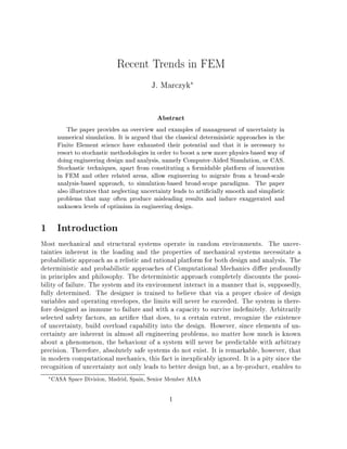
clearly the debility of the deterministic vision of life.
15 16 17 18 19 20 21 22 23 24
96
98
100
102
104
106
108
110
thickness (mm)
frequency(Hz)
Example of unacceptable model-experiment correlation
Figure 3: Multiple experiments versus Monte Carlo Simulation; a typical scenario. Only
in a similar perspective is it possible to assess how the experimental results compare with
those of a numerical simulation. The '+' corresponds to experiment and '.' to simulation.
One may observe in fact two distinct clouds of points, one resulting from a Monte
Carlo Simulation and the other originating from a series of tests. The horizontal axis
corresponds to a design parameter, say thickness, while the vertical axis represents some
engineering quatity of interest, for example frequency of vibration. Clearly, the two clouds,
do not stem from the same phenomenon although they overlap, at least in part. Without
getting into details, intuition suggests that the sine qua non condition for two phenomena
to be judged as similar, or stistically equivalent, is that their clouds have similar shapes
and orientations. Clearly, if two such clouds come in contact only at their borders, or
even if they overlap but have distinct shapes topologies there will be serious evidence of
some major physical discrepancy or inconsistency between the phenomena they portray.
From gure 3 another striking fact emerges, namely that there may exist situations in
which a '+' test lies very close to a '.' simulation and both lie on the edges of two
nearly tangent clouds. These cases, catalogued as accidental or fortuitous correlation,
are extremely dangerous and misleading since a lucky combination of test circumstances
and simulation parameters may prompt an impetuous and unexperienced mesh-man to
14

15. conclude that his simultion has hit the nail on the head.7
Obviously, a single test and a
single simulation can not go further. It is impossible to squeeze out more information from
where it does not exist. It is impossible to say anything on the validity of the numerical
model in a single test-single simulation scenario. Not a single clue on robustness. Not one
hint on con dence or reliability. All we can speak of in similar circumstances is simply
the Euclidean distance between the model and the experiment. What complicates the
situation is the fact that experiments are expensive because prototypes are expensive. A
de nitely better situation is portrayed in gure 4. Here the clouds overlap, have similar
size and orientation. This is, of course, still no guarantee, but we are surely on the right
track.
17 18 19 20 21 22 23 24
94
96
98
100
102
104
106
thickness (mm)
frequency(Hz)
Example of acceptable model-experiment correlation
Figure 4: Example of statistically equivalent populations of tests and analyses. The '+'
corresponds to experiment and '.' to simulation.
5 Conclusions
Statistics is, at least for engineers, part of the lost mathematics, the mathematics now
considered maybe too advanced for high school and too elementary, or useless, for college.
Statistics has been kicked out of many university courses and school curricula. There is in
fact a puzzling and obsessive adversion to statistics in engineering. One of the reasons is
that statistics has been made repugnant and revolting to the student and engineer thanks
to too much epsilonics and not enough examples of practical application, its usefullness
and its tremendous power. Probability, on the other hand, is the mathematics of the
20th century. Its history goes back to the 16th century, but not until the present century
did people fully realize that nature and the real world can be described exhaustively only
7In such cases we prefer to talk of unlucky, rather than lucky, circumstances.
15

16. by laws governing their randomness. Today, High Performance Computing technology,
together with Monte Carlo Simulation techniques, o ers a unique opportunity to push the
FEM science, and CAE in general, into more physics-based domains and to abandon the
idealistic and arti cial vision of life upon which deterministic numerical analysis thrives.
Monte Carlo Simulation is a monument to simplicity and constitutes a phenomenal vehicle
for the incorporation of uncertainty and complexity management in engineering.
References
1 Marczyk, J., editor, Computational Stochastic Mechanics in a Meta-Computing Per-
spective, International for Numerical Methods in Engineering CIMNE, Barcelona,
December, 1997.
2 Klein, M., Schueller, G.I., et. al.,Probabilistic Approach to Structural Factors of Safety
in Aerospace, Proceedings of the CNES Spacecraft Structures and Mechanical Testing
Conference, Paris, June 1994, Cepadues Edition, Toulouse, 1994.
3 Gustafson, J., Computational Ver ability and Feasibility of the ASCI Program, IEEE
Computational Science Engineering, Vol. 5, No. 1, January March, 1998.
16