beven 1996.pdf

HYDROLOGICAL PROCESSES, VOL.6,279-298 (1992)
THE FUTURE OF DISTRIBUTED MODELS: MODEL
CALIBRATION AND UNCERTAINTY PREDICTION
KEITH BEVEN AND ANDREW BINLEY
Centrefor Research on Environmental Systems, Lancaster University, Lancaster, LA1 4YQ, U.K.
ABSTRACT
This paper describes a methodology for calibration and uncertainty estimation of distributed models based on
generalized likelihood measures. The GLUE procedure works with multiple sets of parameter values and allows that,
within the limitationsof a given model structure and errors in boundary conditionsand field observations,different sets
of values may be equallylikely as simulators of a catchment.Procedures for incorporatingdifferent types of observations
into the calibration;Bayesian updating of likelihood values and evaluatingthe value of additional observationsto the
calibration process are described. The procedure is computationally intensive but has been implemented on a local
parallel processing computer.The methodologyis illustrated by an applicationof the Instituteof HydrologyDistributed
Model to data from the Gwy experimental catchment at Plynlimon,mid-Wales.
KEY WORDS Distributed models Calibration uncertainty Likelihood
INTRODUCTION
In a critical discussionof the process of physically-baseddistributed modelling, Beven (1989a)has pointed to
the limitations of the current generation of distributed models and argued that a possible way forward must
be based on the realistic estimation of predictive uncertainty. Beven (1989b) and Binley and Beven (1991)
have outlined a general strategy for model calibration and uncertainty estimation in such complex models.
This strategy is explored further in this paper with a proper exposition o
f the approach, which we call
Generalized Likelihood Uncertainty Estimation (GLUE). The GLUE procedure is placed in the context of
other calibration and uncertainty estimation techniques,and its use is demonstrated by an application to the
Gwy storm runoff data set from the Institute of Hydrology’s experimental catchments at Plynlimon, mid-
Wales which was previously used by Calver (1988) and Binley et al. (1991).
In outlining the basis of the GLUE procedure, Beven (1989b) starts from the premise that prior to the
introduction of any quantitative or qualitativeinformation to a modelling exercise,any model/parameter set
combination that predicts the variable or variables of interest must be considered equally likely as a
simulator of the system. It is further suggestedthat because all model structures must, to some extent, be in
error and that all observations and measurements on which model calibration is based must also be subject
to error, then there is no reason to expectthat any one set of parameter values will represent a true parameter
set (within some particular model structure) to be found by some calibration procedures. Rather, it is
suggested that it is only possible to make an assessment of the likelihood or possibility of a particular
parameter set being an acceptable simulator of the system.We may then assign a likelihood weight to any
model structure/parameter set combination on the basis of the evidenceconsidered. Each likelihood weight
may be based on a number of different sources of evidence, that may include qualitative as well as
quantitative measures.
Such an approach is, of course,different to most calibration procedures used in hydrology,in which some
0885-6087/92/03b279-20$15.00
01992 by John Wiley & Sons Ltd.
Received and accepted 20 May 1991

280 K. BEVEN AND A. BINLEY
global optimum parameter set is sought, and any assessment of parameter and predictive uncertainty is made
with respect to that global optimum. There have been may studies of techniques for facilitating the search for
an optimal parameter set which have illustrated the difficulties of finding such an optimal set in the high-
dimensional parameter space associated with hydrological models (see, for example, Ibbitt and O’Donnell,
1971;Sorooshian and Dracup, 1980;Sorooshian et al., 1983; Gupta and Sorooshian, 1985;Kuczera, 1983;
Hornberger et al,, 1985; Kuczera, 1990).Such difficulties arise from the use of threshold parameters, from
intercorrelation between parameters, from autocorrelation and heteroscedascity in the residuals and from
insensitive parameters, Such effects result in local minima, valleys and plateaux in the parameter response
surface and will lead to difficulties in using either automatic search, random search, or trial and error
calibration techniques. The problems tend to get worse with an increasing number of parameter values. In
the case of physically-based distributed models which inevitably have a large number of parameters and in
which one would expect highly intercorrelated parameters from physical principles, such difficulties will be
experienced in an extreme form.
Indeed, it can be argued that in hydrological systems, equivalence of parameter sets should be expected.
Hydrological terminology recognizes a number of different mechanisms of catchment hydrological response,
including Hortonian or infiltration excess overland flow, saturation excess overland flow, subsurface
stormflow, and throughflow or interflow. It is also recognized that these mechanisms are not mutually
exclusive, but may occur in different parts of a catchment within the same storm, or at a point in the
catchment during different storms depending on rainfall intensities and antecedent conditions. Clearly, any
model that purports to be a general physically-based model of catchment hydrology must have the capability
of predicting storm runoff responses based on all these mechanisms or combinations of them. It might
therefore be possible that a particular storm hydrograph or combination of storm hydrographs might be
predicted by the model, given a suitable combination of parameter values, by different combinations of the
above mechanisms. How then does the hydrologist recognise what might be the ‘correct’ combination of
parameter values, given that the effects of both errors in the model structure and errors in the observed data
must also affect how well the model apparently fits the observations. The answer is, of course, that the
hydrologist might have reason to prefer some combination of parameter values over others (perhaps (s)he
has never seen overland flow in this catchment, although perhaps (s)he may never really have looked), but
there may be many sets of parameter values that are really equally likely as simulators of the system under
study.
At this point it is common practice to choose the set of parameter values that gives the ‘optimal’ fit to the
observed data and, if the modeller is enlightened (for example Goren and Burges, 1981), to calculate an
estimate of the uncertainty bounds around the optimum. This may be a little short sighted in the case of
hydrological models. It might, for example, exclude sets of parameters that give a qualitatively more correct
simulation of the response mechanism in the catchment, but which has parameters in a completely different
part of the parameter space. This is the difficulty of distinguishing between multiple optima in the response
surface. It might also exclude parameter sets distant from the current optimum that, while giving more
accurate results than the current optimum for a different period of observations.
There is a particular problem associated with distributed models in this respect. The sheer number of
parameter values involved has already been noted. Even when the hydrologist is prepared to accept that a
distributed model is predicting the right sort of response mechanism, there may be many different
combinations of the grid element parameters that might lead to equivalently accurate predictions. Without
detailed internal state observations, it may be difficult to distinguish between these equivalent predictions. It
should also be noted that such internal observations will generally be few in number and their value may be
limited by the fact that such measurements are normally made at a much smaller scale than the grid element
scale predictions (see Beven, 1989 for a discussion of this point). In fact, the preliminary work by Wood et al.
(1988, 1990) on trying to assess the scale of an appropriate ‘representative elementary area’ in hydrological
storm response would suggest that at the scale of a small catchment, getting the right pattern of parameter
values may not, in fact, be crucial. However, taking account of the fact that those parameters may have some
distribution function may be important, so that assuming that a catchment can be modelled by an
appropriate homogeneous ‘effective’set of parameter values will lead to significant errors.

DISTRIBUTED MODELS 3: CALIBRATION AND UNCERTAINTY 281
GENERALIZED LIKELIHOOD UNCERTAINTY ESTIMATION (GLUE): AN OVERVIEW
The GLUE procedure recognizes the equivalence or near-equivalence of different sets of parameters in the
calibration of distributed models. It is based upon making a large number of runs of a given model with
different sets of parameter values, chosen randomly from specified parameter distributions. On a basis of
comparing predicted and observed responses, each set of parameter values is assigned a likelihood of being a
simulator of the system. That likelihood may be zero when it is considered that the set of parameter values
gives a behaviour that is not characteristic of the system, either because of the direct comparison with the
available data, or because of conditioning on the basis of some a priori knowledge about the system (e.g.
overland flow has never been seen in the catchment). Note that any interaction between the parameters is not
a problem in this procedure, it will be implicitly reflected in the likelihood values. Different sets of initial and
boundary conditions may also be evaluated in this way, indeed,in the general case,different model structures
can be considered.
We use the term likelihood here in a very general sense, as a fuzzy, belief, or possibilistic measure of how
well the model conforms to the observed behaviour of the system, and not in the restricted sense of maximum
likelihood theory which is developed under specific assumptions of zero mean, normally distributed errors
(Sorooshian and Dracup, 1980; Sorooshian et al., 1983).Our experience with physically-based distributed
hydrological models suggests that the errors associated with even optimal parameter sets are neither zero
mean or normally distributed.
In the GLUE procedure, all the simulations with a likelihood measure significantly greater than zero are
retained for consideration. Rescaling of the likelihood values such that the sum of all the likelihood values
equals 1 yields a distribution function for the parameter sets. It may then be seen that the traditional
calibration search for an optimal parameter set is an extreme case of this procedure in which the ‘optimal’
solution is given a likelihood of 1 and all others are set to zero.
Such likelihood measures may be combined and updated using Bayes theorem (see Box and Tiao, 1973;
Lee, 1989). The new likelihoods may then be used as weighting functions to estimate the uncertainty
associated with model predictions (see below). As more observed data become available, further updating of
the likelihood function may be carried out so that the uncertainty estimates gradually become refined over
time.
The requirements of the GLUE procedure are as follows:
1. A formal definition of a likelihood measure or set of likelihood measures. It is worth noting at this stage
that a formal definitionis required but that the choiceof a likelihood measure will be inherently subjective.
2. An appropriate definition of the initial range or distribution of parameter values to be considered for a
particular model structure.
3. A procedure for using likelihood weights in uncertainty estimation.
4. A procedure for updating likelihood weights recursively as new data become available.
5. A procedure for evaluating uncertainty such that the value of additional data can be assessed.
These requirements will be addressed in the following sections, together with an example application to
modelling the Institute of Hydrology Gwy catchment in Mid-Wales using the Institute of Hydrology
Distributed Model (IHDM).
MODELLING THE GWY CATCHMENT
The IHDM represents a catchment as a seriesof hillslope planes an channel reaches.In the current version of
the IHDM (IHDM4) surface flows on each hillslope and stream channel flow are modelled in a one-
dimensional sense by a kinematic wave equation solved by a finite difference scheme. Subsurface flow, both
saturated and unsaturated is modelled by the two dimensional (vertical slice)Richards equation, incorporat-
ing Darcy’s Law and mass conservation considerations. It is solved by a Galerkin finiteelement scheme with
allowance for varying slope widths and slope angles to account for slope convexity/concavity and
convergence/divergence. Linkages are made between the different flow types: hillslope overland flow can
arise from saturation-excess and/or infiltration-excessof the soil material, and saturated zones within the soil

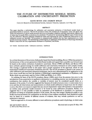
Figure I. The Institute of Hydrology Gwy ExperimentalCatchment, Plynlimon,mid-Wales. (a) Catchment topography.(b) Discretiza-
tion into hillslope and channel elements for use in the Institute of Hydrology Distributed Model
of the lower hillslopes provide lateral flow contributions to the stream system.Further details of the IHDM,
includingdescriptionsof the pre-programsfor determination of effectiveprecipitation,can be found in Beven
et al. (1987).
The Gwy catchment at the head of the River Wye in central Wales has a drainage area of 3.9 km2(Figure
la). It is an upland area of impermeable bedrock, predominantly shallow soils and grassland vegetation
where streamflow is derived from throughflow,natural soil pipe flow and some overland flow. In using the
IHDM on the Gwy catchment,the drainage area was dividedinto five sectionsof hillslopeand three channel
reaches (Figure lb). Ten events were selected for study (see Table I). Five events were treated as calibration
events (storms 1 to 5), the remaining events (storms 6 to 10) were retained for a validation exercise. The
calibration sequence includes four winter events with a recurrence interval of between 1 and 10 years. The
other calibration storm (storm 4 in Table I) was a very large runoff event of 5 August 1973which was of a
magnitudethat caused somegeomorphologicalchanges to hillslopesand channels(Newson, 1980).Its return
Table I. Storm characteristics for the Gwy catchment
~-~ - ~ ~~
Storm Date Total Maximum Peak flow
no. Rainfall intensity (m3
s-I)
(mm) (mmh-')
1
2
3
4
5
6
7
8
9
10
17-19 NOV
81
27-29 Jan 83
11-13Feb 76
5-7 Aug 73
17-19 NOV
78
8-10 Dec 83
13-15Jan 81
19-22 Apr 78
5-7 Oct 80
20-22 JuI 81
80.51
111.44
107.25
121.77
124.18
98.23
94.78
74.91
75.60
55.30
9.17
8.60
10.43
25.66
8.74
8.72
13-34
11.56
5.86
5.54
8.0
6.1
8.5
164*
7.6
1.2
10.5
8.3
3.70
2.21
'Estimated

Table 11. IHDM parameter distributions
Parameter Description Minimum Maximum
Ks Saturated hydraulic conductivity (m h - I) 0.02 2.00
8. Saturated moisture content (m3m-3) 0.15 0.60
Initial soil moisture potential (m) -0.40 -0.05
fin Overland flow roughness coefficient (m0.5
h- ) 50.00 10oO.00
period has been estimated at 50-100 years. This event has been included in the series to study the effect of a
‘non-uniform’ sequence of observed events in the GLUE procedure. The validation sequence consists of
three winter events, which have very similar characteristics to the four winter events in the calibration
sequence,plus two less intensive non-winter events (storms 9 and 10).
Although the IHDM ,in theory, requires a large number of parameter values we have employed the model
in a more practical and typical fashion by recognising uncertainty from only a few parameters (in this case
four) to which the IHDM is considered to the most sensitive.The parameters, which are listed in Table 11,
were considered to be effective values as spatial variability was not treated. The other parameters of the
IHDM were fixed on the basis of field estimates.
DEFINITION OF THE LIKELIHOOD FUNCTION
As with any calibration procedure, the GLUE methodology requires the definition of some measure of
goodness-of-fit,in this case the likelihoodmeasure,in comparing observations and predictions of the model.
The likelihood measure must have some specificcharacteristics.It should be zero for all simulations that are
considered to exhibitbehaviour dissimilarto the system under study,and it should increasemonotonicallyas
the similarity in behaviour increases. These are not restrictive requirements, and could be satisfied by
adapting many of the goodness-of-fitindices used in the past. Some example likelihood measures are:
a) A model efficiency or coefficient of determination defined by
which is zero when the variance of the residuals(
a
:
) is equal to the variance of the observations (of), and one
when the residuals are everywhere zero;
b) The likelihood function used by Binley and Beven (1991)which is also based on the sum of squares of the
residuals as
8,= (O:)-N
where N is a parameter chosen by the user. Note that when N = 0, every simulation will have equal
likelihood and when N + co the singlebest simulation will have a rescaledlikelihood of 1while all others will
have a likelihood of zero.
c) Scaled maximum absolute residual
8,=max[le(t)l];t= 1,..., T (3)
where e(t) is the residual between observed and predicted variables at time t. This type of measure has been
used, for example, by Keesman and van Straten (1989, 1990) and van Straten and Keesman (1991) in
modelling lake eutrophication, with the additional requirement that residual lies within measurement error
bounds (else 9-
= 0). This will generally require, however, that the observed data must be smoothed to
remove outliers; otherwise no parameter sets may give an acceptable simulation under this likelihood

284 K. BEVEN A N D A. BINLEY
definition. They found that it was necessary to make the ‘measurement error bounds’ unduly wide to obtain
a reasonable number of parameter sets that would satisfy this latter criterion at all time steps, an interesting
reflection on the quality of the theory that underlies our mechanistic models of environmental systems. Other
likelihood measures based on the absolute values of the residuals are also possible such as the sum of the
absolute values
LIKELIHOOD FUNCTIONS FOR MULTIPLE OBSERVATIONS
Most studies of calibration procedures in hydrology have examined goodness-of-fit measures based on
observed and predicted discharges (Sorooshian and Dracup, 1980; Hornberger et al., 1985).In the present
context we may also be interested in comparing predictions of internal state variables. Some way of
combining information from different measures of behaviour is therefore required. In this respect, the
approach suggested here has something in common with the conditional simulation used in groundwater
modelling (e.g. Delhomme, 1979)in which uncertainty in the model predictions is estimated by Monte Carlo
simulation conditioned on parameter distributions for the grid elements of the model. Those distributions are
calculated by the kriging of measured values, such that the parameter variances are low close to measurement
points and increase with distance away from the measurement points. This may be considered as a special
case of the procedure proposed here in which the likelihood values are defined a priori on the basis of locally
Gaussian distributions defined by the kriged variances.
For the general case of multiple sites or types of observation contributing to an overall likelihood weight
for each simulation, some way of combining the individual measures of goodness of fit is required. There are
also a number of different ways of doing this. An obvious choice is to use a weighted sum of the individual
measures, for example the likelihood function in Equation 2 becomes:
where: rn is the number of observed responses,
W, is the weight for observationj such that c y = 1,
aij is the error variance of the jth observed variable,
but this has the effect of averaging out the effect of poor performance on one or more measures. This may be
made a dimensionless measure if the weights are chosen to be equal to the variance of the observations.
An alternative automatic weighting procedure for multiple goodness-of-fit criteria has been suggested by
van Straten (1983) as the pseudomaximum likelihood measure
m
for which an appropriate likelihood measure might be
A different function adopted by Klepper el al. (1991) is based on the maximum of the series of model-
observation errors, weighted according to their ‘usefulness’, for each realization. A weighted product of
individual error criterion could also be considered, or if the likelihoods are treated as fuzzy measures of the
set of acceptable simulators of the system, a number of generalized fuzzy set operations could be conisidered.
Given the rn fuzzy or likelihood measures 9&,
9,.
..Y,,,
associated with each realization, we seek to

combine those measures in some way. Two possible ways are:
Set union
Set intersection
Ya
nY 6
n. Z,,,= min[Ya,Y6, ...Y,J
More complex union and intersection operators are described by Klir and Folger (1988).
Again it should be emphasized that there is a considerablesubjectiveelement involved in the choice of the
likelihood function,which should reflectnot only the observations available but also the purposes for which
the model is required. For example, some studies might place great weight on the accuracy with which the
model can predict peak discharges, while others would place much more emphasis on correctly reproducing
the occurrence of saturated conditions at a given level in the soil. The important point is that an explicit
definition of the likelihood function used must be made for each study. It should also be stressed that the
likelihood measureis associatedwith a set of model parameter valuesand, as such,differentsimulations with
very similar values of any single parameter might be associated with a wide range of likelihood values. We
will illustrate this point in the application presented below.
UNCERTAINTY AND MODEL STRUCTURAL ERROR
There are many sources of error in any modelling study: error due to poorly defined boundary conditions
and input data; error associated with measurements used in model calibration; and error due to deficiencies
in model structure. The likelihood weights of the GLUE procedure will reflect all sources of error in the
modelling process and allow the uncertainties associated with those errors to be carried forward into the
predictions.
It would normally be expected that the residuals between the observations and predictions for any
particular simulationmight have structure.In general,those residualswill be biased and autocorrelated with
heteroscedasticvariance (forexampleSorooshian and Dracup, 1980).In what follows,we will take no further
account of the structure of the residuals since the effects of such structure are retained implicitly in the
likelihood weight associated with the parameter set producing that residual sequence.
The result of applying the GLUE procedure is a range of likelihood weight predictions that may be
compared with observed behaviour. We may find, as will be demonstrated below, that the observations with
which model predictions are to be compared may still fall outside the calculated uncertainty limits. If it is
accepted that a sufficiently wide range of parameter values (or even model structures) has been examined,
and the deviation of the observations is greater than would be expected from measurement error, then this
would suggest that the model structure(s) being used, or the imposed boundary conditions, should be
rejected as being inadequate to describe the system under study.
When this is found to be the case, a model can be redeemed by redefining the likelihood function used to
produce wider uncertainty limits(e.g. by reducingthe power N in Equation 2). The importance of an explicit
definition of the likelihood function is then readily apparent as the calculated uncertainty limits will depend
upon the definition used. The modeller can, in consequence, manipulate the estimated uncertainty of his
predictionsby changingthe likelihoodfunction used. At first sight,this would appear to be unreasonable but
we would hope that more careful thought would show that this is not the case, provided that the likelihood
definition used is explicit.After all, if the uncertainty limits are drawn too narrowly, then a comparison with
observations will suggest that the model structure is invalid. If, on the other hand they are drawn too widely,
then it might be concluded that the model has little predictive capability. What we are aiming at is an
estimate of uncertainty that is consistent with the limitations of the model(s) and data used and that allows a
direct quantitative comparison between different model structures. Hopefully, with time and improved

understanding of both system and appropriate model structures, more demanding likelihood measures can
be used and the uncertainty limits will accordingly be drawn more tightly.
It is perhaps worth noting that more traditional techniques of uncertainty estimation in linear statistics are
also dependent upon the definition of likelihood used, although the assumptions of the theory (normally
distributed, uncorrelated, zero mean, constant variance residuals at the most restrictive) are commonly
violated.
PRIOR PARAMETER DISTRIBUTIONS
Given the definition of an appropriate likelihood measure, the next stage in the GLUE procedure is the
definition ofappropriate initial or prior parameter distributions. There may again be a considerable degree of
subjectivity involved at this point. The prior parameter distributions must be broad enough to ensure that
the model behaviours will span the range of observations. This may not always be easy to assess u priori,even
given some physical insight or reasoning. For example, in physically-based distributed models it will be
necessary to specifyhydraulic conductivities for different soil types and soil horizons for each grid element in
the model. Given some information on soil texture or particle size distributions, the estimation procedures
reported by Clapp and Hornberger (1978) or Rawls and Brakensiek (1989)would appear attractive. In those
studies, the mean and standard error of estimation of hydraulic conductivity values can be estimated for
different soil types based on the very large data sets accumulated by the USDA. Some care is in order,
however. The measured hydraulic conductivities used in those studies were carried out on small soil samples
and must be most representative of the soil matrix. The model requires hydraulic conductivity estimates at
the grid element scale,where both mean and variance might be very different (seediscussion in Beven, 1989a,
b). It is therefore probably safest to start with unduly wide ranges of possible parameter values, since the
Bayesian likelihood weighting procedure will refine the range of acceptable parameter sets as more data is
added.
From a Bayesian point of view, we may express the problem of defining these initial parameter
distributions in terms of a set of assumptions reflectingour prior knowledge of the parameter values or, more
normally perhaps, a set of assumptions that is consistent with our lack of prior knowledge about what might
be appropriate values.The prior distributions will consequently often be defined purely subjectively,with the
only requirement of the current procedure being that the resulting distributions should be ‘proper’ in the
sense that the assumed probability density function should integrate to unity. This will normally require that
the modeller must decide on an appropriate prior range of the parameters to be considered together with the
form of the distribution function within that range. In the case of little prior knowledge, a uniform
distribution function over a chosen (wide) range will be appropriate to define a suitable ‘reference’ or
standard prior distribution. The suitability of the chosen range may be evaluated by comparison of the
predicted responses within that range.
The assumption of a locally uniform prior distribution reflecting limited knowledge about appropriate
values of the parameters is a convenient one, but has been the subject of considerable discussion in the
literature of Bayesian statistics (see forexample Box and Tiao, 1973).An important objection, that is relevant
to hydrological modelling, is that a uniform distribution associated with a parameter, 8, may not be uniform
in transformations of 8, i.e. the effect of 8 within the model. Ideally, we would chose a prior distribution
consistent with the effectiveness of changes in a model parameter on changes in model response. For
example, it might be more appropriate to chose a uniform distribution of log-transformed hydraulic
conductivity. This is, of course, consistent with a modeller’sprior knowledge of the sensitivity of a particular
model to different parameter values in different circumstances.
In practice, the assumption of a uniform reference prior, is unlikely to prove critical, because as soon as
information is added in terms of comparisons between observed and predicted responses then, if this
information has value, the distribution of calculated likelihood values should dominate the uniform prior
distribution when uncertainty estimates are recalculated. Estimates of the prior parameter distributions for
the Gwy catchment have been based on the previous experience of modelling this catchment reported in
Binley et ul. (1991). Uniform distributions have been chosen with a range wide enough to encompass the

expected modes of response of the catchment (see Table 11).Again it is emphasizedhere that the procedures
are applied to parameter sets, rather than values of individual parameter values, so that any interactions
between parameters are taken into account implicitly in the procedure.
UNCERTAINTY ESTIMATION
The likelihood value associatedwith a set of parameter values may be treated as a fuzzy measure that reflects
the degreeof belief of the modeller in that set of parameter values (within its particular model structure) as a
simulator of the system. That degree of belief is derived from and may be carried over to the predicted
variables arising from that set of parameter values. Treating the distribution of likelihood values as a‘
probabilisticweightingfunctionfor the predicted variables, therefore allowsan assessmentof the uncertainty
associated with the predictions (conditioned on the definition of the likelihood function, input data and
model structure used). For example at any particular time step, the discharges predicted by each sample
model run may be ranked in order of magnitude and, using the likelihoodweightsassociated with each run, a
distribution function of the predicted dischargesmay be calculated. Some examples are shown in Figure 2.
From this distribution various summary values can be calculated, such as the weighted mean predicted
discharge, the centroid and modal values, the weighted variance and selected quantiles.
Figure 3 shows the results of multiple IHDM simulations of the Gwy catchment hydrograph for storm 1
given a known rainfall record, using parameter sets selected from the specified uniform prior distributions.
Each simulationcan be associated with a likelihood value based on how well it corresponds to the observed
discharge. The likelihood function used here is that defined by Equation 2 above, as used by Binley and
0.3
U
0
r
7 0.2
Y
-
1
._
!
?
s
”
-
= 0.1
0
0.0
(a)
r
0.20 5.70
r0.96
T
11.20 16.70 22.20 27.70 33.20
Discharge (x103
m3 /hr)
, .
1.72 2.47 3.23 3.99
Discharge (x103rn Ihr)
Figure 2. Distribution functionof predicted dischargesfor storm 3 based on a priori likelihood distribution.(a) Distribution at peak
mean f
l
o
w (b) Distribution at end of event

288 K.BEVEN AND A. BINLEY
1
40
0 12 24 36 48 60 72
Time (hr)
Figure 3. A subset of 20 simulations for storm 1
Beven (1991). The cumulative likelihoods are scaled to 1, so that at any time step the discharges associated
with the individual model runs can be expressed as a cumulative distribution function.
Two points are worth noting about this procedure. The first is that, although the distribution of predicted
discharges appears approximately Gaussian at some time steps and other time steps in the same simulation
period it may be highly skewed (Binley et al., 1991). Thus in general the normal calculation of uncertainty
limits as a function of the variance of the predicted values will not be generally applicable. In this study we
have chosen to use the estimates of the 5th and 95th percentiles of the cumulative likelihood distribution as
the uncertainty limits of the predictions, and the centroid as a measure of the modal behaviour. Figure 4
shows the predicted 90 per cent uncertainty limits defined in this way for storm 1.
Secondly,from time step to time step the position of any particular simulation run within the distribution
will vary. A run that overpredicts at one time step may well underpredict at another time step. This should be
z
5 20
c"
:
: 10
c
._
D
0
0 12 24 36 48 60 72
Time lhrl
Figure 4. Predictive uncertainty for storm 1 based on posterior parameterdistribution. Solid line indicates observed flow,dashed line
indicates 5 and 95 per cent simulation limits

expected from the interaction between the individualparameters and the dynamics of the model, but implies
that the uncertainty limits cannot be related directly to a variance of estimation for individual parameter
values. Remember,each likelihood value is associated with a set of parameter values.
We have specificallychosen to avoid the use of single simulation runs to represent, for example,the ‘best
fit’to the observeddata. We wish to avoid the idea that there is one set of parameter values that can,with any
given model structure,represent a catchment area when it isknown that the model structuremust be in error.
UPDATING OF LIKELIHOOD WEIGHTS
The modeller will frequently be in a position of having a continuing input of new observation periods, or
different types of observations that can be utilized to update the likelihood values and estimated
uncertainties.There may be different waysof utilizingsuchdata to refine the model of a particular catchment.
In the past, this has usually been done on a purely ad hoc basis. One advantage of the GLUE procedure
suggested here is that this procedure must be formalized while still accepting that different types of
observation might be given different weight in the modelling procedure.
Recalculation of the distribution function associated with the parameter sets is carried out easily using
Bayes equation in the form (Fisher, 1922):
where go(@)
is the prior likelihood distribution of the parameter sets,
2’JOIy) is the calculated likelihood function of the parameter sets given the set of new observations, y,
and
2‘,,(@y) is the posterior likelihood distribution of the parameter sets.
Bayesequation in this form presupposesthat the likelihooddistribution has a cumulativevalue of unity. It
is particularlyeasy to apply in the caseof the Monte Carlo procedure used here, sinceeach sampleparameter
set is associated with its own prior likelihood,and its own likelihoodfunction value so that Equation 8 can be
applied on a sample by samplebasis. The definition of the distributions will, of course,remain subject to the
sampling limitations of the Monte Carlo procedure.
The updating of the resulting uncertainty limits is demonstrated for the Gwy catchment in Figure 5.
Figures 5b and c show the resulting uncertainty limits on the predicted discharges as calculated using the
prior and posterior likelihood distributions. This shows that there is a slight reduction in uncertainty
associated with taking account of the new observations.The calculated posterior likelihood distribution may
be used to project the uncertainty associated with the predictions forward, and becomes the prior
distribution in Equation 8 when new observationsare available to calculate a new set of values of the chosen
likelihood function. Thus, in a well-posed model with accurate observations we should expect that the
posterior likelihoods should become increasingly constrained as additional observations are considered.
Whether this will also be true of hydrological models and hydrological observations remains to be seen.
Figure 6 showsthe prior and posterior uncertainty limits calculated for the high magnitude event storm 4. In
this case it can be seen that the limits widen. This suggests that the event dependency of the IHDM’s
apparently physically-based parameters will limit the possibility of finding an ‘optimum’ parameter set.
RESAMPLING OF PARAMETER DISTRIBUTIONS
Initial experiencein using the GLUE procedures has revealed that the effect of using the Bayesian updating
procedures described above is to gradually reduce the number of parameter sets that have posterior
likelihood values significantlygreater than zero. This will gradually thereforereduce the sample size defining
the appropriate distributions. This is effectively saying that the area of the parameter space that contains
parameter sets that are acceptable simulators of the catchment becomes increasingly constrained as more
data is taken into account. This would be expected(if a model has any value at all) and in a traditional model
calibration context would indicate that there is a convergence on an optimal set of parameter values. This is

’0°1 -
100
80
$ 60
3
140
20
LOglOlLikelihoodl
4dm
-4.11 -3.71 -3.32
~ -263 -225
~ - 2 9 2 -2.53 -213
LoglOlLikelihoodl
la1
E 301
% I
x 20
0 12 24 36 48
Time lhl
Figure 5. (a) prior and posterior likelihood distributions for storm 3. (b) uncertainty limits for storm 3 calculated using prior likelihood
distribution. (c) uncertainty limits for storm 3 calculated using posterior likelihood distribution after conditioning based on observed
discharges in storm 3
40
0 12 24 38 48 80 12
Time lhrl
Figure 6. (a) Uncertainty limits for storm 4 calculated using prior likelihood distribution; (b) Uncertainty limits for storm 4 calculated
using posterior likelihood distribution after conditioning based on observed discharges in storm 4

0.0
Likeliho$d
( X l o - 1
rn ABOVE 8.0
rn 7.2 - 8.0
8.4 - 7 2
5.6 - 8.4
4.8 - 5.8
4.0 - 4.8
3.2 - 4.0
2.4 - 3.2
1.8 - 2.4
0.8 - 1.8
0.0 - 0.8
0 0.0
-0.1
C
.-
*
-0.2
-0.3
-0.4
0.0 0.5 1.0 1.5 2.0
K s (m/hr)
Figure 7. Variation of the likelihood function, prior to storm 3, with K , and
not necessarily the case here for two reasons. The GLUE procedure explicitlyallows that the ‘optimal’set of
parameter values may vary from period to period of observation and that this will be reflected in the
evolution of the posterior likelihood distribution. It also allows that there may be more than one region of
high likelihood values in the parameter space, as shown in Figure 7, where the likelihood distribution has
been collapsed onto a two parameter space.
There is, as in any multiparameter calibration problem, a certain difficulty in displaying such results. The
GLUE procedure is only sensitive to such complex response surfaces in respect of the number of samples
required to define the likelihood distribution adequately. Again, it is worth emphasising that it only works
with parameter sets,and the display of the distribution for individual parameters has value only in the sense
of evaluating the sensitivityof the model to that parameter. Sensitivityanalysis can be carried out using the
GLUE resultsdirectly using,for example,the GeneralizedSensitivityAnalysisprocedures of Hornberger and
Spear (1981), modified to take account of the likelihood weights for the acceptable simulations. Figure 8
shows such a comparison of the cumulative distributions for the behaviour and non-behaviour simulations
(the definition of which follows) for the IHDM parameters varied in this study after taking account of the
observations from the first storm. This shows a distinct difference between the behavioural and non-
behavioural distributions of 0, and t,bin,which is demonstrated further by the significanceof the Kolmogor-
ov-Smirnoff D statistic in each case (Table 111).
It is important, however, to retain a proper definition of the areas in the response surface with significant
likelihood values as more observations are taken into account. This may be done by excludingthose sets of
parameter values giving simulations with very low likelihood values (the non-behaviour simulations of

K. BEVEN AND A. BINLEY
292
10
0" 0 8
s
c
8 06
-
m
>
3 0 4
i
c3 0 2
0 0
K, lm/hl
1.0
.
t
Bz0.4
5
0 0.2
0.0
Figure 8. Comparison of behavioural(0) and non-behavioural (x) parameter distributions based on likelihoods after storm 1
Hornberger and Spear, 1981)and replacing them with a new set of simulations which are expected to have
significant likelihood values by resampling the response surface.This is done quite easily within the GLUE
procedure since the shape of the likelihood distribution is always defined with respect to a uniform sampling
of values along each parameter axis. For the current purpose this has advantages over the more common
Monte Carlo procedure of taking samplesto reproduce the expected density function in the parameter space,
so that each sample is then equally weighted. Excludinga set of parameter values is equivalent to setting the
likelihood at that point in the parameter space to zero. New sample sets may be added by continuing to
sample uniformly along each axis and interpolating a likelihood valuefrom the posterior distribution defined
by the existing sets of values. If the interpolated value results in a negligiblelikelihood value, a new sample is
taken until the required number of sample parameter sets is available.
This resampling procedure is computationally quite efficient in that new sets of parameter values can be
chosen before the model runs are made. The search area might also be limited if it is clear that there are areas
of the parameter space that are not expected to yield significant likelihood values, but experience would
suggest that excludingsuch areas is difficultif the parameters are considered individually and should only be
done with care. The estimated likelihood values for the resampled parameter sets can be added to the existing
prior likelihood distribution to be used in the next application of the Bayesian updating of Equation 8. They
represent,in effect, our best prior knowledge of the shape of the likelihood distribution before taking account
of any additional observations. In this study we treat all realisations within the lower 5 per cent tail of the
cumulative likelihood distribution as non-behavioural and adopt a simple distance squared interpolation
procedure for resampled, taking account of the 10 nearest neighbours in the parameter space to each
resampled point. All the results presented here have made use of this resampling technique.
MODEL VALIDATION AND PREDICTION WITHIN THE LIMITS OF UNCERTAINTY
The GLUE procedure allows the modeller to be realistic about the uncertainties associated with his
modelling in a way that is conceptually very simpleto understand. The posterior likelihood distribution may
be used directly to evaluate the uncertainty limits for future events for which observed data may not be

-
L
r 10.
5
0.40.
40,
(b)
, I
, I
, .
m
r'h
Time (hr) Time (hr)

Table 111. Kolmogorov-Smirnoff D statistic
calculated for behavioural and non-behavioural
IHDM parameter distributions for storms 1 to
5. Values underlined are significant at the 5 per
cent level
~~
Parameter K , 0s *in f
Storm I 0.076 0497 p
.
6
7
4 0.111
Storm 2 -
0.190 __
0.214 -
0.303 -
0.260
Storm 3 0184 0-129 0.437 0.290
Storm 4 0.354 0.162 0248 0.064
Storm 5 __
0.270 0.185 0323 0.116
available or, in a split sample test, to validate a model by comparison with observed data that have not been
used in the likelihood updating. This has been done for five further storms on the Gwy catchment, using the
posterior likelihood distribution following storm 5. The results are shown in Figure 9 for storms 6, 8 and 9.
The uncertainty bands for storm 8 fail to enclose the minor peak for storm 8 due to inconsistency between
observed precipitation and discharge. Such a feature, which is not uncommon, should be recognized if the
observations of storm 8 were to be used for further refinement of the likelihood distribution.
Physically-based models, such as the IHDM are increasingly being used to predict the results of land-use
and climatic change in a catchment. In general, this has been done by a variation on scenario modelling
without any consideration being given to the uncertainties associated with individual runs of the model (but
see Binley et al., 1991 for an exception in the context of land-use change). If the changed conditions to be
considered involve changing parameters or boundary conditions of the model, then there will clearly be
additional uncertainty associated with the changed conditions relative to a model ‘calibrated’ using the
GLUE procedure to the present condition of the catchment. This will require a subjective definition of prior
likelihood weights associated with the realizations used to model the new catchment condition.
EVALUATING THE VALUE OF ADDITIONAL DATA
The refinement of the uncertainty limits as new data become available provides a measure of the value of that
data in the model calibration, and an opportunity to evaluate the value of different types of data in the
modelling procedure. To do this objectively, requires some measure of the uncertainty associated with the
predictions. The calculated 90 per cent uncertainty limits may not be an adequate measure in this respect,
since it is likely that they will display some sensitivity to the sampling limitations of the Monte Carlo
procedure. Various integral measures of uncertainty are available (seefor example Klir and Folger, 1988),for
example the probabilistic Shannon Entropy measure, H,
where the likelihoods Yi,i = 1, 2,. ..M are scaled such that Epi= 1 and M is the total number of
realizations. This is a maximum ( = log, M ) when all the realizations are equally likely (the case of the
uniform prior distribution). It has a minimum of 0 when one single realization has a likelihood of 1 and all
others have a likelihood of zero (the case of the ‘optimal’ parameter set). The way in which the value of H
changes with the use of more observations will depend upon the specificdefinition of the likelihood function
2
’
;
and the value of the observations in constraining the predictive uncertainty.
A second measure, the U-uncertainty, is classed by Klir and Folger (1988) as a possibilistic measure of

295
DISTRIBUTED MODELS 3: CALIBRATION AND UNCERTAINTY
non-specificity.It is defined as
M
u = 1 (9;
- Ti+
l)log, i
i = 1
where the Ti
are the scaled likelihoodsranked from highest to lowest (with YAn+
= 0 by convention).The
U-uncertainty has a maximum for a uniform distribution ( = log, M) and a minimum of 0 when a single
realization has a likelihood of Tl = 1.
Both the Shannon entropy and U-uncertainty measures are difficult to apply in the current context when
resamplingprocedures gradually increasethe number of realizationsM. We have modified both measuresto
make use of a discretization of the cumulative ranked likelihood function based on M* increments. The
incremental likelihood is calculated by interpolation for each of the M* increments after which both
Equations 9 and 10can be applied in this rescaled form.In the resamplingprocedure we have followedbased
on uniform samplingin the parameter space,it is necessary to keep track of those resampled parameter sets
that are rejected as well as those added to the number of realizationsretained, both add to effectivenumber of
realizations used, even though those rejected are never actually run.
In this study we have evaluated only the utility of additional discharge data in this respect, since only
minimalinternal state data is availablefor the Gwy catchment. Figure 10showsthe change in the uncertainty
measures (9) and (10) calculated with the posterior likelihood distributions after the application of Bayes
equation for each storm. It is worth noting that the uncertainty calculated in this way does not always
decrease with the addition of further information.This should surely be expected with hydrological models,
where further storms with different specifichydrological responses (such as storm 4 in this study), may not
always be reproduced by the same sets of parameter values that have appeared optimal up to that time.
The same procedures may be used to evaluate the value of different types of hydrological data. In
particular, for the distributed models that have been under discussion here, the value of distributed
observations of internal states of the catchment, such as water table levels or soil moisture profiles, can be
considered.Someinitial work reported in Binleyand Beven (1991)using a hypothetical data set suggeststhat
the use of such data may not be straightforward. In particular, such observations are typically point
7-
0 U-Uncertainty
. Shannon EntrcQy
4 measure. H
5-
3 7 , , ,
1 2 3 4 5 6
Slam
Figure 10. Changein estimatedH and U uncertainty measuresbased on the posteriorlikelihoodsfor the sequenceof stormsin TableI.
Likelihood distributionswere discretizedinto M* = 100 increments

observations and, in the same way as measurements of parameter values, may not correspond to the state
variables that are being predicted at the model grid scale. Binley and Beven (1991) suggested that for their
application, the calculated uncertainty values were dominated by limitations in the model structure and
discretisation in reproducing the behaviour of the catchment, rather than the availability of observed data.
COMPUTING REQUIREMENTS
All of the simulations reported here have been run on a parallel computer, the Lancaster University Meiko
Computing Surface, which contains some 80 transputers, each of which provides about 1Mflop average
performance. The GLUE procedure is very easily adapted to a distributed memory parallel processor,
particularly where each realization may be loaded onto a single processor, as was the case with the IHDM. In
general 500 realizations of the IHDM were run for each storm using a 50 transputer array. Each set of runs
for each storm took between 30 and 60 hours of computing time on the 50 processors. There is therefore a
significant computing burden associated with this technique, but one that is not unreasonable even at the
present time. Faster, affordable parallel processing systems, for example based on the Intel i860 (typically 15
or more times the speed of a transputer), are already available. The intention of the GLUE procedure has
been to use this type of computing power in a way that presents highly complex nonlinear calculations to a
user in a conceptually very simple way and with a minimum of assumptions.
THE FUTURE OF DISTRIBUTED MODELS: CRITICAL EXPERIMENTS, VISUALIZATION,
AND QUALITATIVE LIKELIHOOD MEASURES
Looking to the future, we envisage a number of ways that the GLUE procedure might lead to a constructive
evaluation of both model results and data in the process of distributed modelling. Given that the procedure
allows the estimation of the uncertainty associated with a particular set of predictions, we might perhaps
expect that with the current generation of distributed models the uncertainty limits will be large. The
question then arises as to whether the availability of additional data would help to constrain those
uncertainty limits. Within the GLUE framework, this question could be posed in the context of whether there
are (cost effective)critical experiments that would yield likelihood functions which would significantly reduce
the predictive uncertainty, always subject, of course, to the ultimate constraints of model structural error.
Experiments could be designed, for example, to evaluate the relative value of a series of spatial hydraulic
conductivity/transmissivitymeasurements, a number of observation wells in different locations or additional
raingauge sites.
The additional data need not always be quantitative. The advantages of distributed models in producing
distributed predictions can be used to effect by allowing the modeller to evaluate the process responses
predicted by the model in their correct spatial context. Modern visualization techniques on graphics
workstations allow the rapid display of distributed data in a way that allows the pattern of response to be
qualitatively evaluated. A qualitative likelihood measure could be designed in this way, comparing patterns
of response with field understanding and giving zero likelihood to those simulations not considered to
behave in a way consistent with knowledge of field processes. The information content to be processed within
a multiple simulation context is, of course, immense and, rather than a visual evaluation, might require the
initial setting of performance criteria (likelihood measures) based on field understanding even where there
are no direct internal state measurements.
CONCLUDING DISCUSSION
The Generalized Likelihood Uncertainty Estimation (GLUE) procedure described above provides a formal
framework for taking into account some of the particular difficulties associated with the calibration and
application of distributed hydrological models. In particular, the procedure incorporates:
1. The possibility that different sets of parameter values may be equally likely as simulators of a catchment

system within the limitations of a given specific model structure and errors in the definition of boundary
conditions and observed variables;
The expectation that the errors between observed and predicted responses may be biased, non-Gaussian,
autocorrelated, and heteroscedastistic;
The possibility of updating the likelihood weight associated with a particular set of parameter values as
more observations become available by a simple application of Bayes equation;
The possibility of evaluating the value of different types of data by examination of the effect on the
likelihood distribution;
Procedures for evaluating the sensitivityof the model to individual parameter values as an extensionof the
Generalized Sensitivity Analysis of Hornberger and Spear (198I).
The GLUE procedure requires of the modeller two formal definitions in any particular application. These
are:
A. A joint prior distribution of parameter values;
B. A definition of a likelihood function, with appropriate weights for different predicted variables;
In many applications of distributed models in the past such requirements in model calibration have not
been made explicit and this is, we believe a significant feature of the procedures we propose. However, the
reader should note that the use of different definitions should be expected to lead to different results in terms
of the predicted uncertainty limits.
It is also worth noting, finally, that the GLUE procedure allows not only different parameter sets, but also
different model structures to be incorporated into the uncertainty analysis,where by model structure we can
subsume the use of different discretizations or sets of boundary conditions as well as different models. In the
future of distributed modelling, such considerations and the evaluation of predictive uncertainty must be
given prominence in addition to the gradual improvements that we might expect in model definition and the
development of solution techniques.We hope that the GLUE procedure might provide the basis for a proper
technologyfor the formal evaluation of both models and observations. We accept that the application of the
procedure with its requirement of multiple simulations is currently limited by the general availability of
advanced computing facilitiesbut expect this to change over time with the increasing availability of dedicated
parallel processing workstations. In the future we intend to address some of the issues raised in the preceding
text, in particular the use of field measured internal state data in the calibration of distributed models.
ACKNOWLEDGEMENTS
We would like to thank Ann Calver for providing the original Gwy data set and initial IHDM calibrations
together with the past and present staff of the Institute of Hydrology, Llanbrynmair, who have ensured the
collectionof data often under difficultconditions. The ideas contained in this paper have evolved over a long
period of continued, but often confusing,experiment and discussion.We would like to thank those who have
tried to understand what we were getting at and, in doing so, helped clarify and corrent some of our initial
thoughts. The work has been supported by NERC grants GR2/6364 and GR3/7983, SERC Transputer Loan
TR1/064 and a Nuffield Science Research Fellowship awarded to KJB.
REFERENCES
Beven, K. J. 1989a. ‘Changing ideas in hydrology. The case of physically based models’, J. Hydrology, 105, 157-172.
Beven, K. J. 1989b. ‘Interflow’, in Morel-Seytoux, H. J. (Ed.), Unsaturated Flow in Hydrological Modelling, D Reidel, Dordrecht.
Beven, K. J., Calver, A., and Morris, E. M. 1987. ‘The Institute of Hydrology Distributed Model’, Institute of Hydrology Rept. No. 98,
Institute of Hydrology, Oxon, U.K.
Binley, A. M. and Beven, K. J, 1991.‘Physically-based modelling of catchment hydrology:a likelihood approach to reducing predictive
uncertainty’,in Farmer, D. G. and Rycroft, M. J. (Eds), Computer Modelling in the Environmental Sciences,Clarendon Press, Oxford,
Binley, A. M., Beven, K. J., Calver, A., and Watts, L. G. 1991. ‘Changing responses in hydrology: assessing the uncertainty in physically
Box, G. E. P. and Tiao, G. C. 1973. Bayesian Inference in Statistical Analysis, Addison-Wesley, Reading, MA.
Calver, A., 1988. ‘Calibration, sensitivity and validation of a physically-based rainfall-runoff model’, J. Hydrology, 103, 103-115.
75-88.
based model predictions’, Water Resources Research, vol. 27, 1253-1261.

Clapp, R. B. and Hornberger, G. M. 1978. ‘Empirical equations for some soil hydraulic properties’, Water Resources Research, 14,
Delhomme,J. P. 1979.‘Spatial variability and uncertainty in groundwater flow parameters: a geostatistical approach’, WaterResources
Goren, D. G., and Burges, S. J. 1981.‘Approximate error bounds for simulated hydrographs’, J. Hydraul. Diu.,ASCE, 107,1519-1534.
Gupta, V. K. and Sorooshian, S. 1985.‘Therelationship between data and the precision of parameter estimates of hydrologic models’,J.
Guymon, G. L., Harr, M. E., Berg, R. L., and Hromadka, T. V. 11, 1981. ‘A probabilistic-deterministic analysis of one-dimensional ice
Fisher, R. A. 1922. ‘On the mathematic foundations of theoretical statistics’, Phil. Trans. Roy. Soc. London, A, 222, 309-368.
Hornberger, G. M. and Spear, R. C. 1981. ‘An approach to the preliminary analysis of environmental systems’,J. Environ.Manag., 12,
Hornberger, G. M., Beven,K. J., Cosby, B. J., and Sappington, D. E. 1985.‘Shenandoah Watershed Study:calibration of a topography-
based, variable contributing area model to a small forested catchment’, Water Resources Research, 21, 1841-1850.
Ibbitt, R. P. and ODonnell, T. 1971. ‘Fitting methods for conceptual models’, J. Hydraul. Diu., ASCE, 97(HY9), 1331.
Keesman, K. and van Straten, G. 1989,‘Identification and prediction propogation of uncertainty in models’ with bound noise’, Int. J.
Keesman, K. and van Straten, G. 1990. ‘Set membership approach to identification and prediction of lake eutrophication’, Water
Klepper, O., Scholten, H., and Van de Kamer, J. P. G. 1991. ‘Prediction uncertainty in an ecological model of the Oosterschelde
Klir, G. J. and Folger, T. A. 1988. Fuzzy Sets, Uncertainty and Information, Prentice Hall, Englewood Cliffs.
Kuczera, G. 1983.‘Improved parameter inferencein catchment models.2. Combining differentkinds of hydrologic data and testing their
Kuczera, G. 1990. ‘Assessinghydrologic model nonlinearity using response surface plots’, J. Hydrology, 118, 143-162.
Lee, P. M. 1989. Bayesian Statistics: An Introduction, Edward Arnold, London.
Newson, M. D. 1980. ‘The geomorphological effectiveness of floods-a contribution stimulated by two recent events in mid-Wales’,
Rawls, W. J. and Brakensiek, D. L. 1989. ‘Estimation of soil hydraulic properties’, in Morel-Seytoux, H. J. (Ed.), Unsaturated Flow in
Rogers, C.C. M., Beven, K. J., Morris, E. M., and Anderson, M. G. 1985.‘Sensitivityanalysis, calibration and predictive uncertainty of
Rose, K., Smith, E. P., Gardner, R. H., and Bartell, S. M. 1991. ‘Parameter sensitivities,Monte Carlo filtering, and model forecasting
Rosenblueth, E. 1975. ‘Point estimates for probability moments’, Proc. Nut. Acad. Sci. U.S.A.,72(10), 3812-3814.
Sorooshian, S. and Dracup, J. A. 1980. ‘Stochastic parameter estimation procedures for hydrologic rainfall-runoff models: correlated
and heteroscedastic error cases’, WaferResorces Research, 16, 430-442.
Sorooshian, S., Gupta, V. K., and Fulton, J. L. 1983. ‘Evaluation of maximum likelihood parameter estimation techniques for
conceptual rainfall-runoff models: influence of calibration data variability and length on model credibility’, Water Resources
Research, 19, 251-259.
Van Straten, G. 1983. Maximum likelihood estimation of parameters and uncertainty in phytoplankton models, in M. B. Beck and G.
van Straten (Eds) Uncertainty and Forecasting of Water Quality, Springer-Verlag, Berlin, 157-171.
Van Straten, G. and Keesman, K. J. 1991.‘Uncertainty propogation and speculation in projective forecasts of environmental change: a
lake eutrophication example’, J. Forecasting, 10, 163- 190.
Wood, E. F., Sivapalan, M., Beven, K. J., and Band, L. 1988. ‘Effects of spatial variability and scale with implications to hydrologic
modelling’,J. Hydrology, 102, 29-47.
Wood, E. F., Sivapalan, M., and Beven, K. J. 1990. ‘Similarity and scale in catchment storm response’, Reviews Geophysics, 28, 1-18.
601-604.
Research, 15(2), 269-280.
Hydrology, 81, 57.
segregation in a freezing soil column’, Cold Regions Science and Technology, 5, 127-140.
7-18.
Control.,49, 2259-2269.
Resources Res., 26(1 I), 2643-2652.
Estuary’, J. Forecasting, 10, 191-209.
compatibility’, Water Resources Research, 19, 1163-1 172.
Earth Sure Process., 5, 1-16.
Hydrologic Modelling, D. Reidel, Dordrecht, 275-300.
the Institue of Hydrology Distributed Model’, J. Hydrology, 81, 179-191.
under uncertainty’, J. Forecasting, 10, 117-133.

beven 1996.pdf

Recommended

Recommended

More Related Content

Similar to beven 1996.pdf

Similar to beven 1996.pdf (20)

Recently uploaded

Recently uploaded (20)

beven 1996.pdf