â

1. Denavit-Hatenberg Parameters for
Serial Kinematic Robot
Assoc. Prof, Nguyen Truong Thinh
Department of Mechatronics - HCMUTE

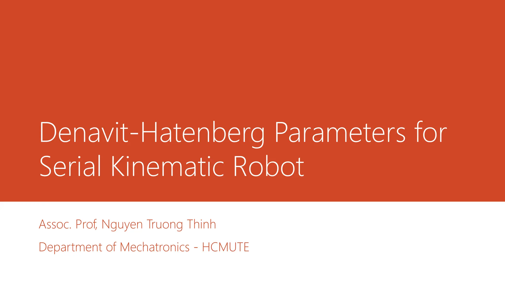
2. INVERSE OF TRANSFORMATION MATIRICES
U H
U R U P
R E P
H E
E T T T T
T T
 
        
1 1 1 1
( )
U U H H U U P H
R R E E R P
H E
R
E
T T T T T T T
T T
   

1 1
U U P H R U P E
R P E E U P E
R
H
H T T T T T T T T
T  
 
known, unknown

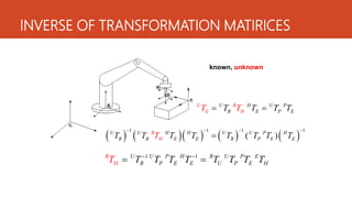
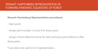
3. DENAVIT-HARTENBERG REPRESENTATION OF
FORWARD KINEMATIC EQUATIONS OF ROBOT
Denavit-Hartenberg Representation procedures:
- Start point:
- Assign joint number n to the first shown joint.
- Assign a local reference frame for each and every joint before or after
these joints.
Y-axis does not used in D-H representation..

4. 2.8 DENAVIT-HARTENBERG REPRESENTATION OF FORWARD
KINEMATIC EQUATIONS OF ROBOT

5. DENAVIT-HARTENBERG REPRESENTATION OF FORWARD
KINEMATIC EQUATIONS OF ROBOT
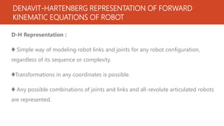
D-H Representation :
♣ Simple way of modeling robot links and joints for any robot configuration,
regardless of its sequence or complexity.
♣Transformations in any coordinates is possible.
♣ Any possible combinations of joints and links and all-revolute articulated robots
are represented.

6. Procedures for assigning a local reference frame to
each joint:
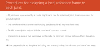
- All joints are represented by a z-axis. (right-hand rule for rotational joint, linear movement for
prismatic joint)
- The common normal is one line mutually perpendicular to any two skew lines.
- Parallel z-axes joints make a infinite number of common normal.
- Intersecting z-axes of two successive joints make no common normal between them (Length is
0.).
Line perpendicular to the plane including two z-axes ( = direction of cross product of two axes)

7. Procedures for assigning a local reference frame to
each joint:
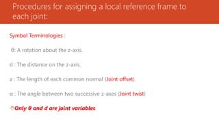
Symbol Terminologies :
θ: A rotation about the z-axis.
d : The distance on the z-axis.
a : The length of each common normal (Joint offset).
α : The angle between two successive z-axes (Joint twist)
Only θ and d are joint variables.

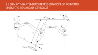
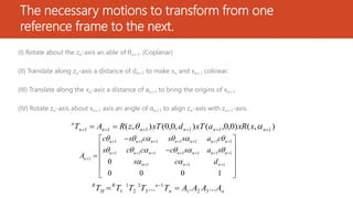
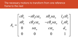
8. The necessary motions to transform from one
reference frame to the next.
(I) Rotate about the zn-axis an able of θn+1. (Coplanar)
(II) Translate along zn-axis a distance of dn+1 to make xn and xn+1 colinear.
(III) Translate along the xn-axis a distance of an+1 to bring the origins of xn+1
(IV) Rotate zn-axis about xn+1 axis an angle of αn+1 to align zn-axis with zn+1-axis.
)
,
(
)
0
,
0
,
(
)
,
0
,
0
(
)
,
( 1
1
1
1
1
1 




 
 n
n
n
n
n
n
n
x
xR
a
xT
d
xT
z
R
A
T 

1 1 1 1 1 1 1
1 1 1 1 1 1 1
1
1 1 1
0
0 0 0 1
n n n n n n n
n n n n n n n
n
n n n
c s c s s a c
s c c c s a s
A
s c d
     
     
 
      
      

  

 
 

 

 
 
 
n
n
n
R
H
R
A
A
A
A
T
T
T
T
T ...
.
... 3
2
1
1
3
2
2
1
1 
 

9. The necessary motions to transform from one reference
frame to the next
0
0 0 0 1
n n n n n n n
n n n n n n n
n
n n n
c s c s s l c
s c c c s l s
A
s c d
     
     
 

 
 

 

 
 
 

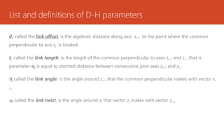
10. List and definitions of D-H parameters
di
: called the link offset, is the algebraic distance along axis zi-1 to the point where the common
perpendicular to axis zi is located.
li called the link length, is the length of the common perpendicular to axes zi-1 and zi , that is
parameter ai is equal to shortest distance between consecutive joint axes zi-1 and zi .
i called the link angle, is the angle around zi-1 that the common perpendicular makes with vector xi-
1,
i called the link twist, is the angle around xi that vector zi makes with vector zi-1.

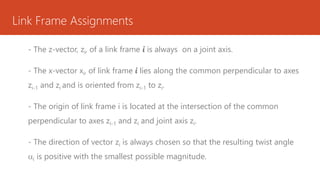
11. Link Frame Assignments
- The z-vector, zi, of a link frame i is always on a joint axis.
- The x-vector xi, of link frame i lies along the common perpendicular to axes
zi-1 and zi and is oriented from zi-1 to zi.
- The origin of link frame i is located at the intersection of the common
perpendicular to axes zi-1 and zi and joint axis zi.
- The direction of vector zi is always chosen so that the resulting twist angle
i is positive with the smallest possible magnitude.

12. Problem 1:
1 2
l1
l2
l3
P
x
y
z
O(xR, yR, zR)
W(0,0,0)

13. Problem 1:
1 2
P
x
y
z
O
W(0,0,0)
z0
z1
x2
x3
x0
x1
z2
z3
# l  d  Var
1 0 /2+1 l1 /2 1
2 0 -/2 l2 /2 L2
3 L3 /2+2 0 0 2

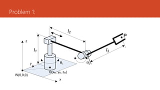
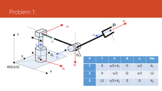
14. Problem 1
1 1
1 1
1
1
cos 0 sin 0
2 2
sin 0 cos 0
2 2
0 1 0
0 0 0 1
A
l
 
 
 
 
 
   
 
   
 
   
 
 
   
  
  
   
   
 
 
 
 
2
2
0 0 1 0
1 0 0 0
0 1 0
0 0 0 1
A
l

 
 

 

 
 
 
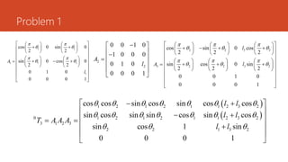
2 2 3 2
2 2 3 2
3
cos sin 0 cos
2 2 2
sin cos 0 sin
2 2 2
0 0 1 0
0 0 0 1
l
l
A
  
  
  
  
 
     
   
     
 
     
 
 
     
  
  
     
     
 
 
 
 
 
 
1 2 1 2 1 1 2 3 2
0 1 2 1 2 1 1 2 3 2
3 1 2 3
2 2 1 3 2
cos cos sin cos sin cos cos
sin cos sin sin cos sin cos
sin cos 1 sin
0 0 0 1
l l
l l
T A A A
l l
      
      
  
   
 
 
 
 
 

 
 

15. Problem 1
 
 
 
 
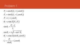
1 2 3 2
1 2 3 2
1 3 2
1
1
2
3
2
2 2
2 2 2
2 3 2
1
cos cos
sin cos
sin
tan 2 ,
sin
cos 1 cos
tan 2 sin ,cos
cos
sin
x
y
z
y x
z
y
P l l
P l l
P l l
a P P
P l
l
a
P
l l
 
 



 
  


 
 
 



  

 

16. Problem 2:
1
2
l1
l3
l4
P
x
y
z
O(xR, yR, zR)
W(0,0,0)
l2

17. Problem 2
1
2
P
x
y
z
O
z0
z1
x2
x3
x0
x1
z2
z3
# l  d  Var
1 0 +1 l1 /2 1
2 l3  l2  l3
3 l4 2 0 0 2

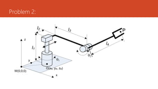
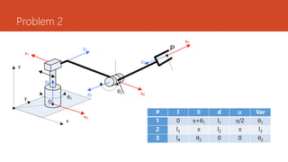
18. Problem 2
1 1
1 1
1
1
cos 0 sin 0
sin 0 cos 0
0 1 0
0 0 0 1
A
l
 
 
 
 
 

 

 
 
 
3
2
2
1 0 0
0 1 0 0
0 0 1
0 0 0 1
l
A
l
 
 
 
 

 

 
 
2 2 4 2
2 2 4 2
3
cos sin 0 cos
sin cos 0 sin
0 0 1 0
0 0 0 1
l
l
A
  
  

 
 
 

 
 
 
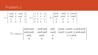
1 2 1 2 1 3 1 2 1 4 1 2
1 2 1 2 1 3 1 2 1 4 1 2
0
3 1 2 3
2 2 1 4 2
cos cos cos sin sin cos l sin cos cos
sin cos sin sin cos sin l cos sin cos
sin cos 0 sin
0 0 0 1
l l
l l
T A A A
l l
        
        
  
  
 
 
   
 
 
 

 
 

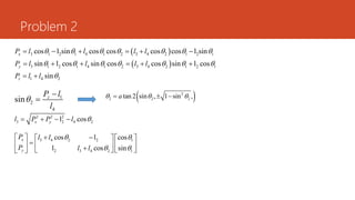
19. Problem 2
 
 
3 1 2 1 4 1 2 3 4 2 1 2 1
3 1 2 1 4 1 2 3 4 2 1 2 1
1 4 2
cos l sin cos cos cos cos l sin
sin l cos sin cos cos sin l cos
sin
x
y
z
P l l l l
P l l l l
P l l
      
      

     
     
 
1
2
4
sin z
P l
l


  
2
2 2 2
tan 2 sin , 1 sin ,
a
  
  
2 2 2
3 2 4 2
l cos
x y
l P P l 
   
3 4 2 2 1
2 3 4 2 1
cos l cos
l cos sin
x
y
P l l
P l l
 
 
 
     

     
  
 
 

20. Problem 3:
l1
l3
l3
l4
5
4
l2
l5
6
z0
z1
z2
z3
z5 º x4
z4
z6
x0
x1
x2
x2
x3
X5
X6

21. Problem 4
E
P
l1
l2
l4
l5
xR, x0
yR, y0
zR
z0
l3
1 2
x1
z1
x2
z2
z3
x3
s

22. Problem 5
l1
l2
l3
l4 l5
l6
l7
l8
P
x0
z0
z1
z2
z3
z4
x2
x1
x3
x4

23. Problem 6
l1
l2
l4
l5
1
2
P
x0
z0
x1
z2
x2
x3
z3
z1

24. Problem 7
zR
xR
yR
x0
x3
1
2
4
l1
l2
l3
l4
l5
l6
R
E
O

25. Problem 8
f
1
2
3
R
xR
yR
zR
l1
l2
l3
l4

26. Thanks for
watching
Industrial Robotics
Find out more at openlab.hcmute.edu.vn