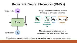
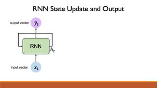
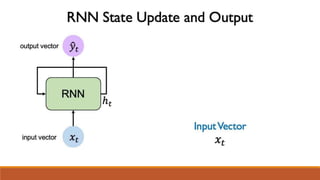
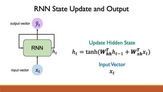
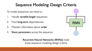
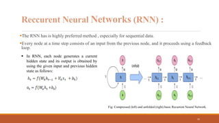
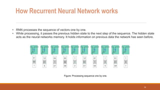
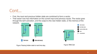
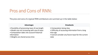
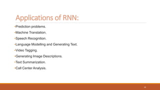
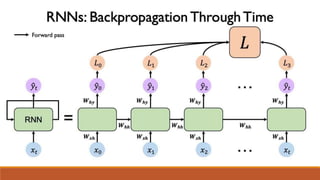
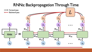
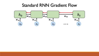
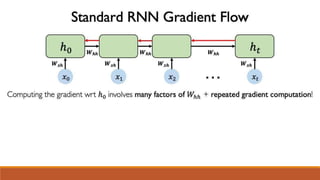
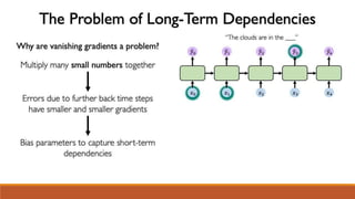
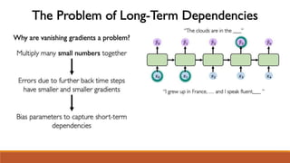
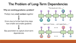
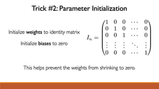
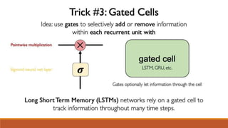
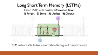
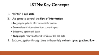
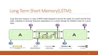
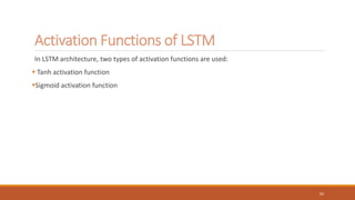
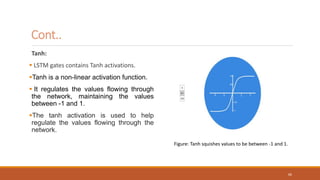
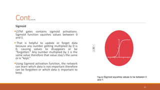
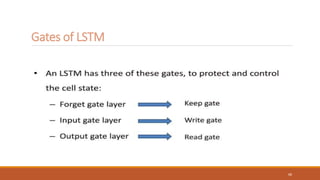
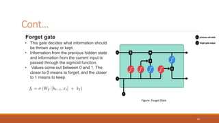
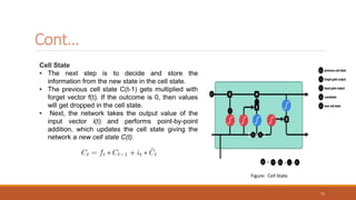
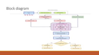
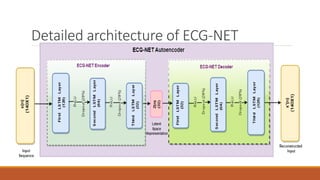
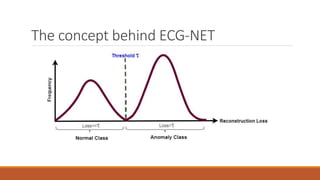
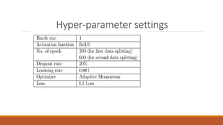
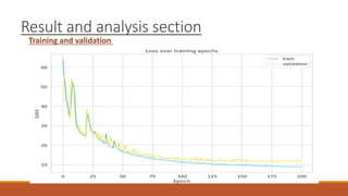
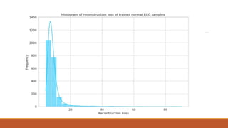
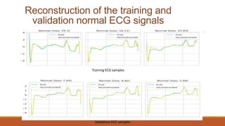
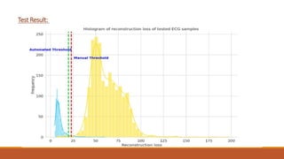
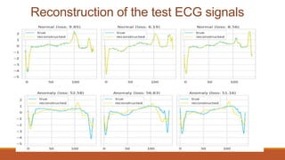
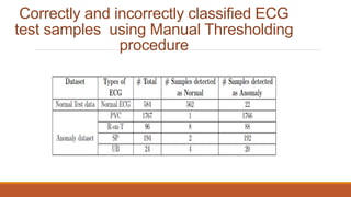
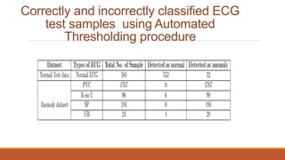
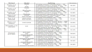
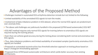
The document discusses recurrent neural networks (RNNs) and long short-term memory (LSTM) networks. It provides an overview of how RNNs work using feedback loops to process sequential data. However, RNNs struggle with long-term dependencies. LSTMs were designed to overcome this by using forget gates to determine what information to keep or forget from the cell state. The document then discusses applications of RNNs and LSTMs like machine translation, speech recognition, and using an LSTM autoencoder for ECG classification. It presents a case study on ECG-NET, an LSTM autoencoder for detecting anomalous ECG signals.


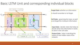
![Input Gate
• The goal of this gate is to determine what new
information should be added to the networks
long-term memory (cell state), given the
previous hidden state and new input data.
• The input gate is a sigmoid activated network
which acts as a filter, identifying which
components of the ‘new memory vector’ are
worth retaining. This network will output a vector
of values in [0,1].
• It is also passed the hidden state and current
input into the tanh function to squish values
between -1 and 1 to help regulate the network.
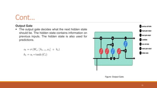
Cont…
Figure: Input Gate.
70](https://image.slidesharecdn.com/rnn-lstm-231025151549-cd5a125a/85/RNN-LSTM-pptx-70-320.jpg)


![[Deck] What's New in Spark-Iceberg Integration via DSV2.pptx](https://cdn.slidesharecdn.com/ss_thumbnails/deckwhatsnewinspark-icebergintegrationviadsv2-260210005337-25955b12-thumbnail.jpg?width=640&height=640&fit=bounds)


