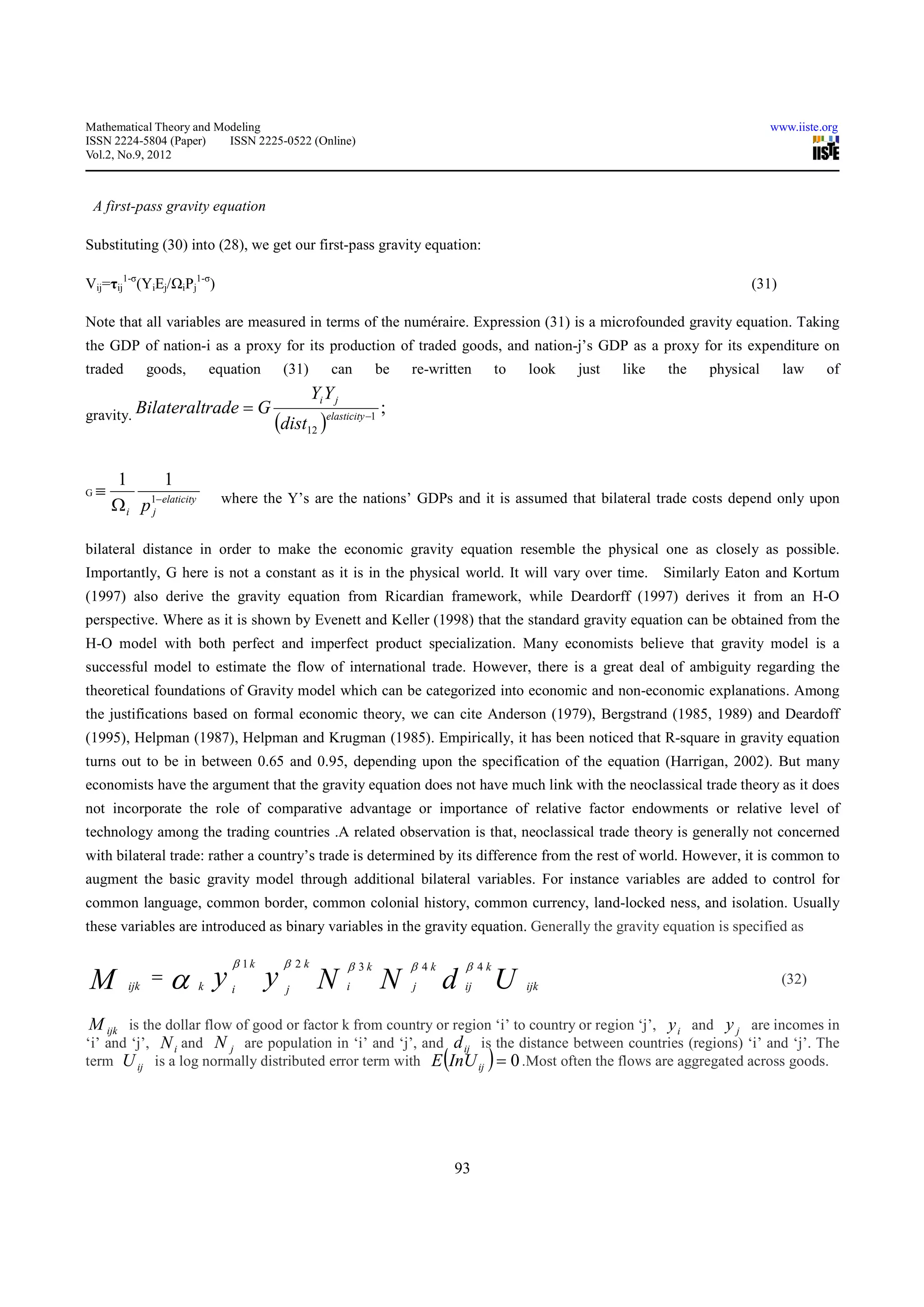
Review of gravity model derivations

Mathematical Theory and Modeling www.iiste.org
ISSN 2224-5804 (Paper) ISSN 2225-0522 (Online)
Vol.2, No.9, 2012

Review of Gravity Model Derivations
Muhammad Tayyab1, Ayesha Tarar 2 and Madiha Riaz3*

1. Assistant Executive Engineer ,Resignalling Project , Pakistan

2. Lecturer at Federal Science College ,Gujranwala ,Pakistan

3. PhD Candidate, School of Social Sciences, University Sains Malaysia

* E-mail of the corresponding author: mdhtarar@gmail.com

Abstract

The gravity model of international trade flows is a common approach to modeling bilateral trade flows. But it is criticized
on the ground of weak theoretical base and poor micro-foundation. The gravity equation for describing trade flows first
appeared in the empirical literature without much serious attempt to justify it theoretically. The theoretical support for the
gravity model was originally very poor, but after the second half of the 1970s, several theoretical developments have filled
this gap .In this study we also endeavor to justify the Gravity model specification and derive gravity equation from different
perspective. We infer from literature and find it a strong empirical tool of analysis for international trade flows even though
of some weakness it innate. Moreover, multilateral trade resistance factors may be added in the empirical estimation to
correctly estimate theoretical gravity model.

Keywords: Gravity Model, Anderson Gravity Model, Tinbergen Gravity Model, Newton’s Basics

1. Introduction

A considerable amount of literature has been published on the gravity model. In early versions of the model, Tin Bergen
(1962) and Poyhonen (1963) conclude that exports are positively affected by income of the trading countries and that
distance can be expected to negatively affect exports. Some studies attempt to add additional structural elements to the
gravity model to better reflect real word observations. A Parallel search of a solid theoretical foundation for the gravity
model addressing several issues related to theoretical weakness has been started since 1970’s. Researchers have examined
the econometric issues of what is the correct way of specifying and estimating a gravity equation, to show how the specific
effects turn out to be significant in empirical analysis. In the last decade, a lot of effort has been made in empirical research
on international trade to explain the bilateral volume of trade through the estimation of a gravity equation [Disdier and Head
(2004)]. As a reminiscence of Isaac Newton's law of gravity, the trade version represents a reduced form which comprises
of supply and demand factors (GDP or GNP and population) as well as trade resistance (geographical distance, as a proxy of
transport costs and home bias) and trade preference factors (preferential trade agreements, common language, common
borders).

Anderson (1979) make the first formal attempt to derive the gravity equation from a model that assume product
differentiation, Bergstrand (1985, 1989) also explore the theoretical determination of bilateral trade in a series of papers, in
which gravity equations are associated with simple monopolistic competition models. Helpman (1987) use a differentiated
product framework with increasing returns to scale to justify the gravity model. Moreover, Deardorff (1995) has proven that
gravity equation characterizes many models and can be justified from standard trade theories.

Anderson and Win coop (2003) derive an operational gravity model based on the manipulation of the CES expenditure
system that can be easily estimated and that helps to solve the so-called border puzzle.

In order to compile the issues of Gravity model we design this study, we are going to discuss the existing literature on
proper econometric specification of the gravity model and its importance for the derivation of bilateral trade flows, vis-à-vis
a healthy appreciation on its modeling and specification.

82

Vol.2, No.9, 2012

2. Derivation of Gravity model

Numerous empirical studies such as Tinbergen (1962) and Linnemann (1966), showed that trade flows follow the physical
principles of gravity: two opposite forces determine the volume of bilateral trade between countries - the level of their
economic activity and income, and the extent of impediments to trade. The latter include in particular transportation costs,
trade policies, uncertainty, cultural differences, geographical characteristics, limited overlap in consumer preference
schemes, regulatory bottlenecks, etc. National borders are among these impediments, even for industrialized countries
(Anderson and van Wincoop, 2003).

Trade potential is the result of matched export capacities and import demands at the microeconomic level. On a more
aggregated level of analysis proximity in demand, per capita income, space, and culture, are key macroeconomic
determinants of export potentials. Thus various combinations of macroeconomic variables, such as gross domestic product
and population with geographic distance, are powerful predictors of trade potentials. Hence, gravity equations have been
used extensively in the empirical literature on international trade (Havrylyshin and Pritchett, 1991; Frankel and Wei, 1993;
Bayoumi and Eichengreen, 1997; Evenett and Hutchinson, 2002). Within this extensive literature, gravity equations share
common features that can be customized for different purposes.

First, a gravity equation is bilateral. It explains a trade-related dependent variable by the combination of macroeconomic
variables, such as country size, income, exchange rates, prices etc., for both countries. Moreover, indicators of
transportation costs between the two countries and more general market access variables are commonly added.

Second, gravity equations can be derived from various theoretical trade models (Deardorff, 1995). Independent from the
underlying trade model chosen, they represent a conditional general equilibrium if multilateral (price) resistance terms are
taken into account. Inference about determinants of trade flows can be drawn due to their property of separability (Anderson
and van Wincoop, 2003). This means that trade flows across countries are separable from the allocation of production and
consumption between countries. Thus, gravity equations establish a link between trade and its determinants conditional on
the observed production and consumption patterns, which draws inference on trade flows from the underlying general
equilibrium structure determining production and consumption allocations. In addition, due to the separability property, the
gravity equation is not affected by the presence of non-tradable sectors in the economy, as non-tradable do not affect the
marginal productivity of tradable goods within a sector (Anderson and van Wincoop, 2003).

Third, a gravity equation may be used in order to estimate either determinants of the volume or determinants of the nature of
trade flows. In the latter case, the purpose is to use an index of intra-industry trade as the dependent variable.

However, there is inevitably a discrepancy between the model applied and the ideal equation that would fit specific
peculiarities of the data well. Border trade, seasonal trade, trade preferences or regional integration may be controlled for
with specific effects by pair of country; such a solution however jeopardizes any attempt to use the model for forecasting
purposes.

Basic Gravity model

The Newtonian physics notion is the first justification of the gravity model. In 1687, Newton proposed the ‘Law of
Universal Gravitation’ which states that the forces of attraction between two objects ‘i’ and ‘j’ is given by

F ij = G
M i M j , (1)
2
D ij

Where notation is defined as follow: Fij is the attractive force, M i and M j are the masses, Dij is the distance
between the two objects and G is a gravitational constant depending on the units of measurement for mass and force.

2.1 GRAVITY MODEL OF TINBERJEN (1962)

83

Vol.2, No.9, 2012

Economists discovered Gravity in trade in 1962, Tinbergen (1962) proposed that roughly the same functional form could be
applied to international trade flows. However, since it has been applied to a whole range of what we might call social
interactions including migration, tourism, and foreign direct investment. The general gravity law for social interaction may
be expressed in roughly the same notation

α β

= G
M M
i j (2)
F ij θ
D ij

where Fij is the” flow” from origin ‘i’ to destination ‘j’ alternatively, M i and M j are the relevant economic sizes of the
two locations. If F is measured as a monetary flow (e.g. export values), then M is usually the gross domestic product (GDP)
or gross national income (GNI) of each location. For flows of people, it is more natural to measure M with the
populations. Dij is the distance between the locations (usually measured from center to center)

2.2 GRAVITY MODEL OF LINNEMANN (1966)

The gravity equation can be analyzed in the light of a partial equilibrium model of export supply and import demand by
Linneman (1966). The study classified factors contributing to trade flows between any pair of countries in three
categories.

a. Factors that indicate total potential supply of country A- the exporting country-to the world market;

b. Factors that indicate total potential demand of country B- the importing country to the world market;

c. Factors that represent the resistance to a trade flow from potential supplier to Potential buyer B.

The resistance factors are cost of transportation, tariff wall, quota, etc.

The potential supply of any country to the world market is linked systematically to(i) The size of a country’s national or
domestic product (simply as a scale factor), and (ii) the size of a country’s population. The level of a country’s per capita
income may also be considered as a third factor though its influence will be very limited, at most. If the third factor indeed
had no effect at all, then the factors (i) and (ii) would obviously be completely independent of each other as explanatory
variables, on theoretical grounds. On the other hand, if the third factor did have an effect, then the three explanatory factors
would not be independent of each other, as a change in one of the three would necessarily be associated with a change in at
least one of the other two variables. For statistical exercises this has important implications because it would imply certain
problems of identification.

In the equilibrium situation potential supply and potential demand on the world market have to be equal. For this, a
prerequisite must be that the exchange rate is fixed at a level corresponding with the relative scarcity of the country’s
currency on the world market. Equality of supply and demand on the world market implies that every country has a
moderate price level in the long run. If the price level is too high or too low, there would be a permanent disequilibrium of
the balance of payments. Adjustment through a change in the exchange rate will necessarily take place. Therefore, the
general price level will not influence a country’s potential foreign supply and demand except in the short-run.

If we assume a constant elasticity of the size of the trade flow in respect of potential supply and potential demand indicating
the trade flow from country ‘i’ to country ‘j’ by Χ ij , the trade flow equation would then combine the three determining
factors in the following way:

Χ ij = β 0
(E ) (M )
i
p β1 p β2
j
(3)
(R ) ij
β3

84

Vol.2, No.9, 2012

Ε ip andΜ p are total potential supply and demand respectively. R is Resistance.Apparently the trade flow from country
j
‘i’to country’j’ will depend on Ε i andΜ j .
p p

In its simplest form, all exponents equal to 1.

The above three explanatory factors in (3) should now be replaced by the variables

determining them. Therefore we now introduce the following notations.

Y= Gross national product

N= Population size

y = Per capita national income (or product)

D = Geographical distance

P = Preferential trade factor

Ε p is a function of Y and N, and possibly of y. Thus we may write

(4)
In which γ1= 1 and γ2 is negative

It was assumed that the same is true for the potential supply Μ which is determined by identical forces.The trade
p

resistance factor R can be replaced by two variables D with a negative exponent and P with a positive exponent. For the
latter variable several other variables may be substituted if we want to distinguish between various types of preferential
trading areas. Here we disregard this complication for the sake of simplicity of the model. Therefore trade flow equation
runs as follows:

Y i δ 1 Y jδ 3 Pijδ 6
X ij = δ o δ
N iδ 2 N δ 4 D ij 5
j
(5)

Where Ρij is various types of preferential trading areas.

2.3 GRAVITY MODEL OF ANDERSON (1979)

The model proposed by Anderson (1979) is mainly based on Cobb-Douglus or CES preference function. Using a trade share
expenditure system, Anderson derives the gravity model, which postulates identical Cobb- Douglas or constant elasticity of
substitution (CES) preference function for all countries and weakly separable utility functions between traded and
non-traded goods. Here utility maximization with respect to income constraint gives traded goods shares that are functions
of traded goods prices only.

Prices are constant in cross-sections; so using the share relationships along with trade balance identity, country ‘j’s imports
of country ‘i’s goods are obtained. Then assuming log linear functions in income and population for shares, the gravity
equation for aggregate imports is obtained. Anderson proposed the following assumptions and derives the Gravity model.

Assumptions:

85

Vol.2, No.9, 2012

• Preferences are homothetic and identical across regions.

• Products are differentiated by place of origin.

• Pure expenditure system is such that the share of national expenditure accounted for by spending on tradable is a
stable unidentified reduced form function of income and population.

Suppose, each country is completely specialized in the production of its own good. So there is one good for each country.
There are no tariffs or transport costs. The fraction of income spent on the production of country ‘i’ is denoted by bi and
is the same in all countries. This implies identical Cobb-Douglas preferences everywhere. Prices are constant at equilibrium
values and units are chosen such that they are all unity with cross-section analysis. Consumption of good ‘i’ (in value and
quantity terms) in country ‘j’ (imports of good ‘i’ by country ‘j’) is thus

M ij = bi Y j (7)

Where Y j is income in country ‘j’.

The requirement that income must equal sales implies that

Yi = bi (∑ j Y j ) (8)

Where bi is the fraction of income spent on production of country ‘i’.

Solving (8) for bi and substituting into (7) we obtain

Yi Y j
M ij = (9)
∑Yj

This is the simplest form of “gravity” model. If error structure is disregarded, a generalization of equation (9) can be
estimated by OLS, with exponents on Yi , Y j unrestricted. In a pure cross section, the denominator is an irrelevant scale
term. The income elasticity produced should not differ significantly from unity.

An unrestricted gravity equation is obtained if Cobb-Douglas expenditure system for traded- non traded goods split is
added. Traded goods shares of total expenditure differ widely across regions and countries. Per capita income is considered
as exogenous demand side factor, and population (country size) is considered a supply-side factor. Trade share should
increase with per capita income and decrease with size. Taking the trade-share function as stable, the expenditure system
model combines with it to produce the gravity equation.

Suppose, all countries produce a traded and a non-traded good. The overall preference function assumed in this formulation
is weakly separable with respect to the partition between traded and non-traded goods: U = u (g (traded goods), non traded
goods). Then given the level of expenditure on traded goods, individual traded goods’ demands are determined as if a
homothetic utility function in traded goods alone g( ) is maximized subject to a budget constraint involving the level of
expenditure on traded goods. The individual traded goods shares of total trade expenditure with homotheticity are functions
of traded goods prices only. To make it simple, it is assumed that g( ) has the Cobb-Douglas form. Since preferences are
identical, expenditure shares for any goods are identical across countries within the class of traded goods. So for any

86

Vol.2, No.9, 2012

consuming country ‘j’, θ i is the expenditure on country i’s tradable good divided by total expenditure in j on tradable; i.e.
θ i is an exponent of g ( ). Let φ j be the share of expenditure on all traded goods in total expenditure of country j and
(
φ j = F Yi , N j . )
Demand for i’s tradable good in country ‘j’ (j’s imports of i’s good) is

M ij = θ iφ j Y j (10)

The balance of trade relation for country i implies that

Yi Φ i = (∑ Y j φ J )θ i (11)

Value of imports of ‘i’ Value of exports of ‘i’

Plus domestic spending = Plus domestic spending

on domestic tradable on domestic tradable

solving (11) for θ i and substituting into (10) we have

= φ Yφ Y = φ Yφ Y
i i j j i i j j

M ij
∑φ Y ∑ ∑ M j j ij
j j i

(12)

A log-linear form of equation (12) is the deterministic form of the gravity equation with the distance term suppressed and a
scale term added. In the same way, the gravity equation can be derived assuming either perfect competition or monopolistic
market structure.

2.4 GRAVITY MODEL UNDER MONOPOLISTIC COMPETITION

Anderson and Wincoop (2003) presented an important and novel analysis , assuming CES-preferences, symmetric trade
barriers and imposing the general equilibrium constraint for trade, i.e. that total sales equal total production, Anderson and
Wincoop explicitly derive the following gravity equation for bilateral trade,

(13)

Here Χ ij is exports from country (region) i to country j, Yi is the income (GDP) of country i, Υ w is the world GDP, t ij
is the trade barrier factor (inverse of one minus the ad valorem tax per unit of exports) between countries (regions) i and j,
assumed to be the same as t ji , and Pi is aggregate trade resistance, or simply, the consumer price index of country i. The
parameter σ is the elasticity of substitution between imports from various origins. The import demand functions in country j,
j = 1… N, are derived from a CES utility function for aggregate consumption D j .

87

Vol.2, No.9, 2012

(14)
Here Q ij is the volume of exports from country i to j, a ij ’s the country-specific positive preference (distribution)
parameters summing to unity and σ is, again, the elasticity of substitution between imports from various origins. The import
demand functions are then

(15)

Where Ρij the price is set by the exporters of country i in the market of country j, inclusive of the cost of trade barriers and,
being dual to the quantity index (14), Pj represents the CES price index of the consumption basket in country j

, (16)

From (16) we can derive the market share of the value of exports Χ ij = Ρij Q ij in country j, in relation to its GDP,
yielding

(17)

Where Y j is the GDP (in nominal terms) of country j and the budget constraint Y j = Pj D j is imposed.

We next consider the export supply decision of a monopolistic firm of country i in the market of country j. For this we need
to specify that aggregate demand D j , which is given by the function

(18)

Where b j is a scale factor representing the size of the country concerned. Note that typically ε < σ. Let there
be K i identical exporting firms in country i. The optimal supply decision of an exporter in country i
maximizing profit in market j is given by

(19)
88

Vol.2, No.9, 2012

Where C i is the marginal cost of production in country i and Qikj denotes the volume of exports of firm k of country i
in the market of country j, t ij is as in equation (13), the trade barrier factor between countries (regions) i and j, and ε
( z i , z j ) denotes the elasticity of the variable z i with respect to the variable z j .

Using (15), (18) and the general result from index number theory i.e. the market share of exporter k in the market of country
j, and summing over the identical K i firms, we derive the following from (19),

(20)
Here h j is the conjectural variation parameter in the proportional output game1 (see Smith and Venables,1988 and
Alho,1996) and s ij is the aggregate market share of country i in the market of country j, i.e.

The supply equation (20) allows for price discrimination between various export markets.

Note that under perfect competition, the export price only depends on the unit cost and the respective trade barrier. But
otherwise under imperfect competition, the larger the country, measured by the number of firms, the lower will be the
export price that firms charge.

We next need a model for the determination of the cost levels C i and therefore introduce the following framework. Assume
simply that labour L is the only factor of production and that there are constant returns to scale, Qi = Ai Li , where Q is the
volume of GDP. Let the utility function U of workers be:

where ν > 0 and Di is total supply. Now optimizing under the budget constraint Pi Di = Wi Li + π i , where W is the wage

rate and π aggregate profits, we derive the result for wage formation,

(21)

Wi
In the next step, in deriving the unit cost C i = , we could take two approaches.
Ai

1
The parameter h j is in relative terms the output response by the competitors to a 1% rise in the output of the firm concerned in market j. if h j is set to
be zero, we have the case of Cournet competition.
89

Vol.2, No.9, 2012

First, we could take it that technology, as incorporated in the parameter A, is identical in all the
countries. But, this assumption of uniformity is not very sensible. Therefore, we allow for differences in
Qi Y
productivities and write Ai, being the average labor productivity, as Ai = = i 2. So, we derive for the unit cost
Li Pi Li

(22)

Where ν is positive and depends simply on the price level in the country and positively on the size of the country measured

by the labor force, which is captured below by population .We further assume that that the average size Q of the firms is

identical in all the countries, so that Ki Q = Qi = Yi/Pi. Then normalize this average size to unity and insert this result and

(22) into (20). By equating export demand (16) with supply (20), we can then solve for export price Pij from the

equilibrium condition,

(23)

Next insert this equilibrium solution (23) for the export price in market j into the export demand equation (17).

Using the approximation that log( x + y ) ≈ log( x ) + log( y ) + o ( x 2 ) + o ( y 2 ) . We can solve for the bilateral exports to

be as follows, returning back to a power function specification,

(24)

The parameter µ is positive and smaller than unity, if the elasticity of substitution σ is greater than unity. In addition,
function (24) includes higher order terms for Yi, Pi and Pj. The parameter h is assumed to be uniform in all market

The above model gives the specification of Gravity model under monopolistic competition, which exists in the whole world.

2
Note that as aggregate demand is identically Equationual to aggregate supply (GDP), i.e. Pi Q Qi = Pi Di
Pi is the price on GDP. These prices Pi Q and Pi are identical.
Q

90

Vol.2, No.9, 2012

2.5 FIRST-PASS GRAVITY EQUATION FOR BILATERAL TRADE

The expenditure share identity

The first step is the expenditure share identity for a single good exported from the ‘origin’ nation to the ‘destination’ nation
is

Pijxij= Shareij Ej (25)

(where Xij is the quantity of bilateral exports of a single variety from nation ‘i’ to nation ‘j’, Pij is the price of the good
inside the importing nation also called the ‘landed price’, i.e. the price of the imported good that is faced by customers in the
importing nation; this is measured in terms of the numeraire. Of course, this makes xij pij the value of the trade flow

measured in terms of the numeraire. Ε j is the destination nation’s expenditure (again measured in terms of the numeraire)

on goods that compete with imports, i.e. tradable goods. By definition, shareij is the share of expenditure in nation j on a
typical variety made in nation-i.

The expenditure function

Microeconomics tells us that expenditure shares depend upon relative prices and income levels. The expenditure share is
assumed to depend only on relative prices. Adopting the CES demand function and assuming that all goods are traded, the
imported good’s expenditure share is linked to its relative price by:

1−σ
 Pij 
( )(
1
, wherePj ≡ ∑ k =1 nk ( p kd )
1−σ
Shareij ≡   R 1−σ ) ,σ > 1 (26)
 Pj 
 

Where pij/Pj is the ‘real price’ of pij. Also, Pj is nation-j’s ideal CES price index (assuming all goods are traded), ‘R’ is the
number of nations from which nation-j buys things (this includes itself), and σ is the elasticity of substitution among all

varieties (all varieties from each nation are assumed to be symmetric for simplicity); n k is the number of varieties

exported from nation k. We assume symmetry of varieties by source- nation to avoid introducing a variety index. As
always, all prices here are measured in terms of the numéraire. Combining (25) and (26) yields product specific import
expenditure equation

Adding the pass-through equation

The landed price in nation-j of goods produced in nation-i are linked to the production costs in nation-i, the bilateral

mark-up, and the bilateral trade costs via p ij = µ i p iτ ij (27)

Where p i is the producer price in nation-i, µ is the bilateral markup and τij reflects all trade costs, natural and manmade.

This assumes that the price-cost markup is a parameter. To keep things simple, we take µ = 1.
91

Vol.2, No.9, 2012

Aggregating across individual Varieties

We have exports of individual varieties. To get total bilateral exports from ‘i’ to ‘j’, we multiply the expenditure share

functions across the number of symmetric varieties that nation ‘i’ has to offer, namely ‘ n i ’. Using upper case V to indicate

to total value of trade, we have

Vij ≡ ni sij Ε j And Vij=ni (piτij)1-σ Ej/Pj1-σ (28)

Lacking data on the number of varieties n i and producer prices p j , we compensate by turning to nation-i’s general

equilibrium condition.

General equilibrium in the exporting nation

Using general equilibrium in the exporting nation to eliminate the nominal price the producer price p i in the exporting

nation-i must adjust such that nation-i can sell all its output, either at home or abroad. Expression (28) gives us nation-i sales
to each market.

Summing over all markets, including i’s own market, we get total sales of nation-i goods. Assuming markets clear, nation
i’s wages and prices must adjust so the nation-i’s production of traded goods equals its sales of trade goods.

In symbols, this requires. Yi = ∑ d =1 Vij , where Yi is nation-i’s output measured in terms of the numéraire.
R

Relating Vij to underlying variables with (28), the market clearing condition for nation-i becomes:

 1 Ej 
Yi = ni p i1−σ ∑ d =1 τ ij−σ 1−σ 
R
(29)

 pj 

where the summation is over all markets (including i’s own market). Solving this for ni pi1−σ will yields,

Yi  1 E 
ni pi1−σ = whereΩ i ≡ ∑ iR=1 τ ij−σ 1−iσ 
 (30)
Ωi  pi  

Here Ω i measures the market potential.

A nation’s market potential is often measured by the sum of its trade partners’ real GDPs divided by bilateral distance. The
capital-omega is a used for ‘openness’ since it measures the openness of nation-i’s exports to world markets.

92

Vol.2, No.9, 2012

A first-pass gravity equation

Substituting (30) into (28), we get our first-pass gravity equation:

Vij=τij1-σ(YiEj/ iPj1-σ) (31)

Note that all variables are measured in terms of the numéraire. Expression (31) is a microfounded gravity equation. Taking
the GDP of nation-i as a proxy for its production of traded goods, and nation-j’s GDP as a proxy for its expenditure on
traded goods, equation (31) can be re-written to look just like the physical law of
Yi Y j
gravity. Bilateraltrade = G ;
(dist12 )elasticity −1

1 1
G ≡ 1− elaticity where the Y’s are the nations’ GDPs and it is assumed that bilateral trade costs depend only upon
Ωi p j

bilateral distance in order to make the economic gravity equation resemble the physical one as closely as possible.
Importantly, G here is not a constant as it is in the physical world. It will vary over time. Similarly Eaton and Kortum
(1997) also derive the gravity equation from Ricardian framework, while Deardorff (1997) derives it from an H-O
perspective. Where as it is shown by Evenett and Keller (1998) that the standard gravity equation can be obtained from the
H-O model with both perfect and imperfect product specialization. Many economists believe that gravity model is a
successful model to estimate the flow of international trade. However, there is a great deal of ambiguity regarding the
theoretical foundations of Gravity model which can be categorized into economic and non-economic explanations. Among
the justifications based on formal economic theory, we can cite Anderson (1979), Bergstrand (1985, 1989) and Deardoff
(1995), Helpman (1987), Helpman and Krugman (1985). Empirically, it has been noticed that R-square in gravity equation
turns out to be in between 0.65 and 0.95, depending upon the specification of the equation (Harrigan, 2002). But many
economists have the argument that the gravity equation does not have much link with the neoclassical trade theory as it does
not incorporate the role of comparative advantage or importance of relative factor endowments or relative level of
technology among the trading countries .A related observation is that, neoclassical trade theory is generally not concerned
with bilateral trade: rather a country’s trade is determined by its difference from the rest of world. However, it is common to
augment the basic gravity model through additional bilateral variables. For instance variables are added to control for
common language, common border, common colonial history, common currency, land-locked ness, and isolation. Usually
these variables are introduced as binary variables in the gravity equation. Generally the gravity equation is specified as

β 1k β 2k β 3k β 4k β 4k
M ijk
= α y k i
y j N i N j d ij U ijk
(32)

M ijk is the dollar flow of good or factor k from country or region ‘i’ to country or region ‘j’, y i and y j are incomes in
‘i’ and ‘j’, N i and N j are population in ‘i’ and ‘j’, and d ij is the distance between countries (regions) ‘i’ and ‘j’. The
( )
term U ij is a log normally distributed error term with E InU ij = 0 .Most often the flows are aggregated across goods.

93

Vol.2, No.9, 2012

Conclusion

From above discussion we deduce that Gravity equation is derivable in different conditions under different assumptions. So
gravity model is usable to measure bilateral trade flows in all types of market structure and conditions. There are different
categories of empirical applications of the Gravity equation, which can be mentioned to investigate issues in international
trade: that are estimating the cost of a border, explaining trade patterns, identifying effects related to regionalism and lastly
tabulating trade potentials. Because of its appeal as an empirical strategy the application of gravity model is becoming
enormously popular. Quoting Eichengreen and Irwin (1997), the gravity model is nowadays "... the workhorse for empirical
studies ..." in international trade. Since the early 1990s, the large availability of international data necessary to fill the
standard specification of the model, the relative independence from different theoretical models, and a bandwagon effect
make the gravity model the empirical model of trade flows (Evenett and Keller, 2002).

References

Anderson, J.E (1979), “A Theoretical Foundation for the Gravity Equation”, The American Economic Review, Vol. 69: 106-16.
Anderson, J.E. and Wincoop E. V (2003), “Gravity with Gravitas: A Solution to the Border Puzzle”, The American Economic Review, Vol. 93, issue 1, pp.
170-92, Nashville.
Bergstrand J.H (1989), “The Generalized Gravity Equation, Monopolistic Competition, and the Factor Proportion Theory in International Trade”, Review
of Economics and Statistics: 143-53.
Bergstrand, J.H 1985, “The Gravity Equation in International Trade: Some Microeconomic Foundations and Empirical Evidence”, The Review of
Economics and Statistics, Vol. 67: 474-81. Harvard University Press.
Deardorff, A. (1997), “Determinants of Bilateral Trade: Does Gravity Work in a Classical World?”, In The Regionalization of the World Economy, ed. by
Jeffrey Frankel. Chicago: University of Chicago Press.
Egger, P. and Pfaffermayr, M (2000), “The Proper Econometric Specification of the Gravity Equation: A Three Way Model with Bilateral Interaction
Effects”, Working Paper, Austrian Institute of Economic Research, Vienna, Austria.
Evenett, S.J. and Keller, W (1998), “On the Theories Explaining the Success of the Gravity Equation”, in NBER Working Paper, No. 6529, Cambridge,
MA: National Bureau of Economic Research.
Frankel, J. and Wei, S.J (1993), “Emerging Currency Blocs”, Mimeo, University of California- Berkeley.
Frankel, J.A. (1997), “Regional Trading Blocs in the World Economic System”, Institute for International Economics, Washington, D.C.
Helpman, E and Krugman, P. (1985), “Market Structure and Foreign Trade”, Cambridge, MA: MIT Press.
Hummels, D. and Levinsohn, J (1993), “Product Differentiation as a Source of Comparative Advantage”, American Economic Review, Papers and
Proceedings, LXXXIII: 445-49.
Head,K. and Mayer. T (2000), “Non-Europe: The Magnitude and Causes of Market Fragmentation in the EU”, Weltwirtschaftliches Archiv, 136(2):
285-314.
Harris, Mark N and Lázlo Mátyás (1998) “ The Econometrics of Gravity Models”, Working Paper No. 5/98, Melbourne Institute of Applied Economic and
Social Research.
Head, K (2003), “Gravity for Beginners”, University of British Columbia, Vancouver. Hummels, D (1999), “Have international transport costs declined?”
working paper.
Krugman, P. (1979), “Increasing Returns, Monopolistic Competition, and International Trade”, Journal of International Economics, Vol. 9: 469-479.
Linder, S. B. (1961), “ An Essay on Trade and Transformation”, New York: John Wiley and Sons.
Linneman, H. (1966), “ An Econometric Study of International Trade Flows”, North Holland, Amsterdam.
Mátyás, L. (1997), “Proper Econometric Specification of the Gravity Model”, The World
Economy, Vol. 20, No3.
Oguledo, V.I. and Macphee, C.R. (1994), “Gravity Models: A Reformulation and an Application to Discriminatory Trade Arrangements”, Applied
Economics, 26: 107-120.
Paas, T. (2000), “Gravity Approach for Modeling Trade Flows between Estonia and the Main Trading Partners”, Working Paper, No. 721, Tartu University
Press, Tartu.
Poyhonen, P. (1963), “Toward A General Theory of International Trade”,Ekonomiska Samfundets Tidskrift, Tredje serien, Argang 16: 69-77.
Rauch, J.E (1996), “Networks Versus Markets in International Trade”, Working Paper 5617, National Bureau of Economic Research.
Rauch, James E. and Trindade, V (2002), “Ethnic Chinese Networks in International Trade" ,Review of Economics and Statistics, 84:1 pp. 116-130.

94

Vol.2, No.9, 2012

Santos Silva J.M.C. and Tenreyro S (2004), “The Log of Gravity”, FRB Boston Series, paper no.03-1 (2003).
Sachs, J.D and Andrew.M.W (1995),“ Natural Resource Abundance and Economic Growth”, Working Paper 5398, National Bureau of Economic
Research.
Tinbergen, J. (1962),” Shaping the World Economy: Suggestions for an International Economic Policy”. The Twentieth Century Fund, New York.

95

This academic article was published by The International Institute for Science,
Technology and Education (IISTE). The IISTE is a pioneer in the Open Access
Publishing service based in the U.S. and Europe. The aim of the institute is
Accelerating Global Knowledge Sharing.

More information about the publisher can be found in the IISTE’s homepage:
http://www.iiste.org

The IISTE is currently hosting more than 30 peer-reviewed academic journals and
collaborating with academic institutions around the world. Prospective authors of
IISTE journals can find the submission instruction on the following page:
http://www.iiste.org/Journals/

The IISTE editorial team promises to the review and publish all the qualified
submissions in a fast manner. All the journals articles are available online to the
readers all over the world without financial, legal, or technical barriers other than
those inseparable from gaining access to the internet itself. Printed version of the
journals is also available upon request of readers and authors.

IISTE Knowledge Sharing Partners

EBSCO, Index Copernicus, Ulrich's Periodicals Directory, JournalTOCS, PKP Open
Archives Harvester, Bielefeld Academic Search Engine, Elektronische
Zeitschriftenbibliothek EZB, Open J-Gate, OCLC WorldCat, Universe Digtial
Library , NewJour, Google Scholar

Review of gravity model derivations

More Related Content

Viewers also liked

Similar to Review of gravity model derivations

More from Alexander Decker

Review of gravity model derivations