Credit Value Adjustment in the Extended Structural Default Model

978–0–19–954678–7 12-Lipton-c12-drv Lipton-Rennie (Typeset by SPi, Chennai) 406 of 657 September 20, 2010 10:30
OUP UNCORRECTED PROOF – PROOF, 20/9/2010, SPi
c h a p t e r 12
................................................................................................................
credit value
adjustment in the
extended structural
default model
................................................................................................................
alexander lipton and artur sepp
1 Introduction
................................................................................................................................................
1.1 Motivation
In view of the recent turbulence in the credit markets and given a huge outstanding
notional amount of credit derivatives, counterparty risk has become a critical issue for
the financial industry as a whole. According to the most recent survey conveyed by
the International Swap Dealers Association (see <www.isda.org>), the outstanding
notional amount of credit default swaps is $38.6 trillion as of 31 December 2008 (it
has decreased from $62.2 trillion as of 31, December 2007). By way of comparison,
the outstanding notional amount of interest rate derivatives was $403.1 trillion, while
the outstanding notional amount of equity derivatives was $8.7 trillion. The biggest
bankruptcy in US history filed by one of the major derivatives dealers, Lehman
Brothers Holdings Inc., in September of 2008 makes counterparty risk estimation and
management vital to the financial system at large and all the participating financial
institutions.
The key objective of this chapter is to develop a methodology for valuing the coun-terparty
credit risk inherent in credit default swaps (CDSs). For the protection buyer
(PB), a CDS contract provides protection against a possible default of the reference
name (RN) in exchange for periodic payments to the protection seller (PS) whose
magnitude is determined by the so-called CDS spread. When a PB buys a CDS from
a risky PS they have to cope with two types of risk: (a) market risk which comes

credit value adjustment 407
directly from changes in the mark-to-market (MTM) value of the CDS due to credit
spread and interest rate changes; (b) credit risk which comes from the fact that PS
may be unable to honour their obligation to cover losses stemming from the default
of the corresponding RN. During the life of a CDS contract, a realized loss due to the
counterparty exposure arises when PS defaults before RN and, provided that MTM
of the CDS is positive, the counterparty pays only a fraction of the MTM value of the
existing CDS contract (ifMTMof the CDS is negative to PB, this CDS can be unwound
at its market price).
Since PB realizes positive MTM gains when the credit quality of RN deteriorates
(since the probability of receiving protection increases), their realized loss due to PS
default is especially big if the credit quality of RN and PS deteriorate simultaneously
but PS defaults first. We define the credit value adjustment (CVA), or the counterparty
charge (CC), as the maximal expected loss on a short position (protection bought) in
a CDS contract.
In order to describe CVA in quantitative rather than qualitative terms, in this
chapter we build a multi-dimensional structural default model. Below we concentrate
on its two-dimensional (2D) version and show that the evaluation of CVA is equivalent
to pricing a 2D down-and-in digital option with the down barrier being triggered
when the value of the PS’s assets crosses their default barrier and the option rebate
being determined by the value of the RN’s assets at the barrier crossing time. We also
briefly discuss the complementary problem of determining CVA for a long position
(protection sold) in a CDS contract.
Traditionally, the par CDS spread at inception is set in such a way that the MTM
value of the contract is zero.1 Thus, the option underlying CVA is at-the-money, so
that its value is highly sensitive to the volatility of the RN’s CDS spread, while the
barrier triggering event is highly sensitive to the volatility of the PS’s asset value. In
addition to that, the option value is sensitive to the correlation between RN and PS.
This observation indicates that for dealing with counterparty risk we need to model
the correlation between default times of RN and PS as well as CDS spread volatilities
for both of them. It turns out that our structural model is very well suited to accomplish
this highly non-trivial task.
1.2 Literature overview
Merton developed the original version of the so-called structural default model (Mer-ton
1974). He postulated that the firm’s value V is driven by a lognormal diffusion
and that the firm, which borrowed a zero-coupon bond with face value N and matu-rity
T, defaults at time T if the value of the firm V is less than the bond’s face
1 Subsequent to the so-called ‘big bang’ which occurred in 2009, CDS contracts frequently trade on
an up-front basis with fixed coupon.

408 a. lipton & a. sepp
value N. Following this ioneering insight, many authors proposed various extensions
of the basic model (Black and Cox 1976; Kim and Ramaswamy, and Sundaresan
1993; Nielsen, and Saa-Requejo, and Santa-Clara 1993; Leland 1994; Longstaff and
Schwartz 1995; Leland and Toft 1996; Albanese and Chen 2005) among others. They
considered more complicated forms of debt and assumed that the default event may
be triggered continuously up to the debt maturity. More recent research has been
concentrated on extending the model in order to be able to generate the high short-term
CDS spreads typically observed in the market. It has been shown that the latter
task can be achieved either by making default barriers curvilinear (Hyer et al. 1998;
Hull and White 2001; Avellaneda and Zhou 2001), or by making default barriers
stochastic (Finger et al. 2002), or by incorporating jumps into the firm’s value dynamics
(Zhou 2001a; Hilberink and Rogers 2002; Lipton 2002b; Lipton, Song, and Lee 2007;
Sepp 2004, 2006; Cariboni and Schoutens 2007; Feng and Linetsky 2008).
Multi-dimensional extensions of the structural model have been studied by several
researchers (Zhou 2001b; Hull and White 2001;Haworth 2006;Haworth Reisinger, and
Shaw 2006; Valu˘zis 2008), who considered bivariate correlated log-normal dynamics
for two firms and derived analytical formulas for their joint survival probability;
Li (2000), who introduced the Gaussian copula description of correlated default times
in multi-dimensional structural models; Kiesel and Scherer (2007), who studied a
multi-dimensional structural model and proposed a mixture of semi-analytical and
Monte Carlo (MC) methods for model calibration and pricing.
While we build a general multi-dimensional structural model, our specific efforts
are aimed at a quantitative estimation of the counterparty risk. Relevant work on the
counterparty risk includes, among others, Jarrow and Turnbull (1995), who developed
the so called reduced-form default model and analysed the counterparty risk in this
framework; Hull and White (2001), Blanchet-Scalliet and Patras (2008), who modelled
the correlation between RN and the counterparty by considering their bivariate corre-lated
lognormal dynamics; Turnbull (2005), Pugachevsky (2006), who derived model-free
upper and lower bounds for the counterparty exposure; Jarrow and Yu (2001),
Leung and Kwok (2005) who studied counterparty risk in the reduced-form setting;
Pykhtin and Zhu (2006), Misirpashaev 2008), who applied the Gaussian copula for-malism
to study counterparty effects; Brigo and Chourdakis (2008), who considered
correlated dynamics of the credit spreads, etc.
Our approach requires the solution of partial integro-differential equations (PIDE)
with a non-local integral term. The analysis of solution methods based on the Fast
Fourier Transform (FFT) can be found in Broadie-Broadie and Yamamoto (2003),
Jackson and Jaimungal, and Surkov (2007), Boyarchenko and Levendorski (2008),
Fang and Oosterlee (2008), Feng and Linetsky (2008), and Lord et al. (2008).
The treatment via finite-difference (FD) methods can be found in Andersen and
Andreasen (2000), Lipton (2003), d’Halluin, Forsyth, and Vetzal (2005), Cont and
Voltchkova (2005), Carr and Mayo (2007), Lipton, Song, and Lee (2007), Toiva-nen
(2008), and Clift and Forsyth (2008).

1.3 Contribution
In this chapter, we develop a novel variant of the one-dimensional (1D), two-dimensional
(2D), and multi-dimensional structural default model the assumption
that firms’ values are driven by correlated additive processes. (Recall that an additive
process is a jump-diffusion process with time-inhomogeneous increments.) In order
to calibrate the 1D version of our structural model to the CDS spread curve observed in
themarket, we introduce jumps with piecewise constant intensity. We correlate jumps
of different firms via aMarshall-Olkin inspiredmechanism (Marshall and Olkin 1967).
This model was presented for the first time by Lipton and Sepp (2009).
In this chapter, we develop robust FFT- and FD-based methods for model cali-bration
via forward induction and for credit derivatives pricing via backward induc-tion
in one and two dimensions. While the FFT-based solution methods are easy to
implement, they require uniform grids and a large number of discretization steps.
At the same time, FD-based methods, while more complex, tend to provide greater
flexibility and stability. As part of our FD scheme development, we obtain new explicit
recursion formulas for the evaluation of the 2D convolution term for discrete and
exponential jumps. In addition, we present a closed-form formula for the joint survival
probability of two firms driven by correlated lognormal bivariate diffusion processes
by using the method of images, thus complementing results obtained byHe, Keirstead,
and Rebholz, (1998), Lipton (2001), and Zhou (2001b) via the classical eigenfunction
expansionmethod. As always, themethod of images works well for shorter times, while
the method of eigenfunction expansion works well for longer times.
We use the above results to develop an innovative approach to the estimation of
CVA for CDSs. Our approach is dynamic in nature and takes into account both
the correlation between RN and PS (or PB) and the CDS spread volatilities. The
approaches proposed by Leung and Kwok (2005), Pykhtin and Zhu (2006), andMisir-pashaev
(2008) do not account for spread volatility and, as a result, may underesti-mate
CVA. Blanchet-Patras consider a conceptually similar approach; however, their
analytical implementation is restricted to lognormal bivariate dynamics with constant
volatilities, which makes it impossible to fit the term structure of the CDS spreads
and CDS option volatilities implied by the market (Blanchet-Scalliet and Patras 2008).
Accordingly, the corresponding CVA valuation is biased. In contrast, our model can
be fitted to an arbitrary term structure of CDS spreads and market prices of CDS and
equity options. The approach by Hull and White (2001) uses MC simulations of the
correlated lognormal bivariate diffusions. In contrast, our approach assumes jump-diffusion
dynamics, potentially more realistic for default modelling, and uses robust
semi-analytical and numerical methods for model calibration and CVA valuation.
This chapter is organized as follows. In section 2 we introduce the structural default
model in one, two, and multi-dimensions. In section 3 we formulate the generic
pricing problem in one, two and multi-dimensions. In section 4 we consider the
pricing problem for CDSs, CDS options (CDSOs), first-to-default swaps (FTDSs),
and the valuation problem for CVA. In section 5 we develop analytical, asymptotic,

410 a. lipton & a. sepp
and numerical methods for solving the 1D pricing problem. In particular, we describe
MC, FFT, and FD methods for solving the calibration problem via forward induction
and the pricing problem via backward induction. In section 6 we present analytical
and numerical methods for solving the 2D pricing problem, including FFT and FD
methods. In section 7 we provide an illustration of our findings by showing how to
calculate CVA for a CDS on Morgan Stanley (MS) sold by JP Morgan (JPM) and a
CDS on JPM sold by MS.We formulate brief conclusions in section 8.
2 Structural model and default event
................................................................................................................................................
In this section we describe our structural default model in one, two, and multi-dimensions.
Qt
2.1 Notation
Throughout the chapter, we model uncertainty by constructing a probability space
(Ÿ,F, F,Q) with the filtration F = {F(t), t ≥ 0} and a martingale measure Q. We
assume that Q is specified by market prices of liquid credit products. The operation
of expectation under Q given information set F(t) at time t is denoted by E[·]. The
imaginary unit is denoted by i, i =
√
−1.
The instantaneous risk-free interest rate r (t) is assumed to be deterministic; the
corresponding discount factor, D(t, T) is given by:
D(t, T) = exp

−

T
t
r (t)dt

(1)
It is applied at valuation time t for cash flows generated at time T, 0 ≤ t ≤ T ∞.
The indicator function of an event ˆ is denoted by 1ˆ:
1ˆ =

1 ifˆ is true
0 ifˆ is false (2)
The Heaviside step function is denoted by H(x),
H(x) = 1{x≥0} (3)
the Dirac delta function is denoted by δ(x); the Kronecker delta function is denoted by
δn,n0 .We also use the following notation
{x}
+ = max{x, 0} (4)
We denote the normal probability density function (PDF) by n (x); and the cumu-lative
normal probability function by N(x); besides, we frequently use the function
P (a, b) defined as follows:

P(a, b) = exp

ab + b2/2

N(a + b) (5)
2.2 One-dimensional case
2.2.1 Asset value dynamics
We denote the firm’s asset value by a(t). We assume that a(t) is driven by a 1D jump-diffusion
under Q:
da(t) = (r (t) − Ê(t) − Î(t)Í)a(t)dt + Û(t)a(t)dW(t) + (e j − 1)dN(t) (6)
where Ê(t) is the deterministic dividend rate on the firm’s assets, W(t) is a standard
Brownian motion, Û(t) is the deterministic volatility, N(t) is a Poisson process inde-pendent
of W(t), Î(t) is its intensity, j is the jump amplitude, which is a random
variable with PDF ( j ); and Í is the jump compensator:
Í =

0
−∞
e j( j )d j −1 (7)
To reduce the number of free parameters, we concentrate on one-parametric PDFs
with negative jumps which may result in random crossings of the default barrier. We
consider either discrete negative jumps (DNJs) of size −Ì, Ì 0, with
( j) = δ( j + Ì), Í = e−Ì −1 (8)
or exponential negative jumps (ENJs) with mean size 1
Ì , Ì 0, with:
( j) = ÌeÌj , j 0, Í =
Ì
Ì + 1
− 1 = − 1
Ì + 1
(9)
In our experience, for 1Dmarginal dynamics the choice of the jump size distribution
has no impact on the model calibration to CDS spreads and CDS option volatilities,
however for the joint correlated dynamics this choice becomes very important, as we
will demonstrate shortly.
2.2.2 Default boundary
The cornerstone assumption of a structural default model is that the firm defaults
when its value crosses a deterministic or, more generally, random default boundary.
The default boundary can be specified either endogenously or exogenously.
The endogenous approach was originated by Black and Cox (1976) who used it to
study the optimal capital structure of a firm. Under a fairly strict assumption that the
firm’s liabilities can only be financed by issuing new equity, the equity holders have the
right to push the firm into default by stopping issuing new equity to cover the interest
payments to bondholders and, instead, turning the firm over to the bondholders. Black
and Cox (1976) found the critical level for the firm’s value, below which it is not optimal
for equity holders to sell any more equity. Equity holders should determine the critical
value or the default barrier by maximizing the value of the equity and, respectively,

412 a. lipton a. sepp
minimizing the value of outstanding bonds. Thus, the optimal debt-to-equity ratio and
the endogenous default barrier are decision variables in this approach. A nice review of
the Black-Cox approach and its extensions is given by Bielecki and Rutkowski (2002),
and Uhrig-Homburg (2002). However, in our view, the endogenous approach is not
realistic given the complicated equity-liability structure of large firms and the actual
relationships between the firm’s management and its equity and debtholders. For
example, in July 2009 the bail-out of a commercial lender CIT was carried out by
debtholders, who proposed debt restructuring, rather than by equity holders, who had
no negotiating power.
In the exogenous approach, the default boundary is one of the model parameters.
The default barrier is typically specified as a fraction of the debt per share estimated
by the recovery ratio of firms with similar characteristics. While still not very realistic,
this approach is more intuitive and practical (see, for instance, Kim and Ramaswamy,
and Sundaresan 1993; Nielsen, and Saa-Requejo, and Santa-Clara 1993; Longstaff and
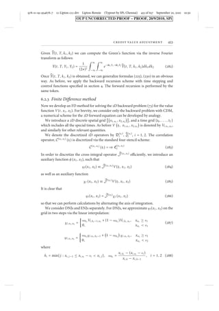
Schwartz 1995; etc.).
In our approach, similarly to Lipton (2002b); and Stamicar and Finger (2005), we
assume that the default barrier of the firm is a deterministic function of time given by
l (t) = E (t)l (0) (10)
where E (t) is the deterministic growth factor:
E (t) = exp

t
0
(r (t) − Ê(t))dt

(11)
and l (0) is defined by l (0) = RL(0), where R is an average recovery of the firm’s
liabilities and L(0) is its total debt per share. We find L(0) from the balance sheet
as the ratio of the firm’s total liability to the total common shares outstanding; R is
found from CDS quotes, typically, it is assumed that R = 0.4.
2.2.3 Default triggering event
The key variable of the model is the random default time which we denote by Ù. We
assume that Ù is an F-adapted stopping time, Ù ∈ (0,∞]. In general, the default event
can be triggered in three ways.
First, when the firm’s value is monitored only at the debt’s maturity time T, then
the default time is defined by:
Ù =

T, a(T) ≤ l (T)
∞, a(T) l (T) (12)
This is the case of terminal default monitoring (TDM) which we do not use below.
Second, if the firm’s value is monitored at fixed points in time, {tdm
}m=1,. . .,M,
0 td
1 . . . tdM
≤ T, then the default event can only occur at some time tdm
. The
corresponding default time is specified by:

Ù = min{tdm
: a(tdm
) ≤ l (tdm
)}, min{} = ∞ (13)
This is the case of discrete default monitoring (DDM).
Third, if the firm’s value is monitored at all times 0 t ≤ T, then the default
event can occur at any time between the current time t and the maturity time T. The
corresponding default time is specified by:
Ù = inf{t, 0 ≤ t ≤ T : a(t) ≤ l (t)}, inf{} = ∞ (14)
This is the case of continuous default monitoring (CDM).
The TDM assumption is hard to justify and apply for realistic debt structures.
The DDM assumption is reasonably realistic. Under this assumption, efficient
quasi-analytical methods can be applied in one and two dimensions under the log-normal
dynamics (Hull and White 2001) and in one dimension under jump-diffusion
dynamics (Lipton 2003; Lipton, Song, and Lee 2007; Feng and Linetsky 2008). Numer-ical
PIDE methods for the problem with DDM tend to have slower convergence rates
than those for the problem with CDM, because the solution is not smooth at default
monitoring times in the vicinity of the default barrier. However, MC-based methods
can be applied in the case of DDM in a robust way, because the firm’s asset values need
to be simulated only at default monitoring dates. Importantly, there is no conceptual
difficulty in applying MC simulations for the multi-dimensional model.
In the case of CDM closed-form solutions are available for the survival probability
in one dimension (see e.g. Leland 1994; Leland and Toft 1996) and two dimensions
(Zhou 2001b) for lognormal diffusions; and in one dimension for jump-diffusions
with negative jumps (see e.g. Zhou 2001a; Hilberink and Rogers 2002; Lipton 2002b;
Sepp 2004, 2006). In the case of CDM, numerical FD methods in one and two
dimensions tend to have a better rate of convergence in space and time than in the
case of DDM. However, a serious disadvantage of the CDM assumption is that the
corresponding MC implementation is complex and slow because continuous barriers
are difficult to deal with, especially in the multi-dimensional case.
Accordingly, CDM is useful for small-scale problems which can be solved without
MC methods, while DDM is better suited for large-scale problems, such that semi-analytical
FFT or PIDE-based methods can be used to calibrate the model to marginal
dynamics of individual firms andMC techniques can be used to solve the pricing prob-lem
for several firms. In our experience, we have not observed noticeable differences
between DDM and CDM settings, provided that the model is calibrated appropriately.
We note in passing that, as reported by Davidson (2008), the industry practice is to use
about 100 time steps with at least 60 steps in the first year in MC simulations of deriv-atives
positions to estimate the counterparty exposure. This implies weekly default
monitoring frequency in the first year and quarterly monitoring in the following years.
2.2.4 Asset value, equity, and equity options
We introduce the log coordinate x(t):
x(t) = ln

a(t)
l (t)

(15)

and represent the asset value as follows:
a(t) = E (t)l (0)e x(t) = l (t) e x(t) (16)
where x(t) is driven by the following dynamics under Q:
dx(t) = Ï(t)dt + Û(t)dW(t) + j dN(t) (17)
x(0) = ln

a(0)
l (0)

≡ Ó, Ó 0
Ï(t) = −1
2
Û2(t) − Î(t)Í
We observe that, under this formulation of the firm value process, the default time
is specified by:
Ù = min{t : x(t) ≤ 0} (18)
triggered either discretely or continuously. Accordingly, the default event is deter-mined
only by the dynamics of the stochastic driver x(t).
We note that the shifted process y(t) = x(t) − Ó is an additive process with respect
to the filtration F which is characterized by the following conditions: y(t) is adapted
to F(t), increments of y(t) are independent of F(t), y(t) is continuous in probability,
and y(t) starts from the origin, Sato (1999). The main difference between an additive
process and a Levy process is that the distribution of increments in the former process
is time dependent.
Without loss of generality, we assume that volatility Û(t) and jump intensity Î(t) are
piecewise constant functions of time changing at times {tc
k
}, k = 1, . . . , k:
Û(t) =
k
k=1
Û(k)1{tc
k−1t≤tc
k
} + Û(k)1{ttc
k
} (19)
Î(t) =
k
k=1
Î(k)1{tc
k−1t≤tc
k
} + Î(k)1{ttc
k
}
where Û(k) defines the volatility and Î(k) defines the intensity at time periods (tc
k−1, tc
k ]
0 = 0, k = 1, . . . , k. In the case of DDM we assume that {tc
with tc
k
} is a subset of {tdm
}, so
that parameters do not jump between observation dates.
We consider the firm’s equity share price, which is denoted by s (t), and, following
Stamicar and Finger (2005), assume that the value of s (t) is given by:
s (t) =

a(t) − l (t) = E (t)l (0)

e x(t) − 1

= l (t)

e x(t) − 1

, {t Ù}
0, {t ≥ Ù} (20)
At time t = 0, s (0) is specified by themarket price of the equity share. Accordingly, the
initial value of the firm’s assets is given by:
a(0) = s (0) + l (0) (21)

It is important to note that Û(t) is the volatility of the firm’s assets. The volatility of
the equity, Ûeq(t), is approximately related to Û(t) by:
Ûeq(t) =

1 +
l (t)
s (t)

Û(t) (22)
As a result, for fixed Û(t) the equity volatility increases as the spot price s (t) decreases
creating the leverage effect typically observed in the equity market. The model with
equity volatility of the type (22) is also know as the displaced diffusion model, which
was introduced by Rubinstein (1983).
2.3 Two-dimensional case
To deal with the counterparty risk problem, we need to model the correlated dynamics
of two ormore credit entities. We consider two firms and assume that their asset values
are driven by the following stochascic differential equations(SDEs):

dai (t) = (r (t) − Êi (t) − Íi Îi (t))ai (t) dt + Ûi (t) ai (t)dWi (t) +
e ji −1
ai (t)dNi (t)
(23)
where
Íi =

0
−∞
e jii ( ji )d ji −1 (24)
jump amplitudes ji has the same PDF i ( ji ) as in the marginal dynamics, jump
intensities Îi (t) are equal to the marginal intensities calibrated to single-name CDSs,
volatility parameters Ûi (t) are equal to those in the marginal dynamics, i = 1, 2. The
corresponding default boundaries have the form:
li (t) = Ei (t) li (0) (25)
where
Ei (t) = exp

t
0
(r (t) − Êi (t))dt

(26)
In log coordinates with
xi (t) = ln

ai (t)
li (t)

(27)
we obtain:
dxi (t) = Ïi (t)dt + Ûi (t)dWi (t) + jidNi (t) (28)
xi (0) = ln

ai (0)
li (0)

≡ Ói , Ói 0
Ïi (t) = −1
2
Û2
i (t) − Íi Îi (t)

The default time of the i -th firm, Ùi , is defined by
Ùi = min{t : xi (t) ≤ 0} (29)
Correlation between the firms is introduced in two ways. First, standard Brownian
motions W1(t) and W2(t) are correlated with correlation Ò. Second, Poisson processes
N1(t), N2(t) are represented as follows:
Ni (t) = N{i } (t) + N{1,2} (t) (30)
where N{1,2} (t) is the systemic process with the intensity:
Î{1,2}(t) = max{Ò, 0} min{Î1(t), Î2(t)} (31)
while N{i }(t) are idiosyncratic processes with the intensities Î{i }(t), specified by:
Î{1}(t) = Î1(t) − Î{1,2}(t), Î{2}(t) = Î2(t) − Î{1,2}(t) (32)
This choice, which is Marshall-Olkin (1967) inspired, guarantees that marginal distri-butions
are preserved, while sufficiently strong correlations are introduced naturally.
Expressing the correlation structure in terms of one parameter Ò has an advantage
for model calibration. After the calibration to marginal dynamics is completed for
each firm, and the set of firm’s volatilities, jump sizes, and intensities is obtained, we
estimate the parameter Ò by fitting themodel spread of a FTDS to a givenmarket quote.
It is clear that the default time correlations are closely connected to the instanta-neous
correlations of the firms’ values. For the bivariate dynamics in question, we
calculate the instantaneous correlations between the drivers x1(t) and x2(t) as follows:
ÒDNJ
12 =

1,2}Ì1Ì2
Û+ Î1ÌÛ22
21
21
+ Î2Ì22
, ÒENJ
12 =

1,2}/(Ì1Ì2)
Û+ 2Î1/ÌÛ22
21 21
+ 2Î2/Ì22
(33)
where we suppress the time variable. Here ÒDNJ
12 and ÒENJ
12 are correlations for DNJs and
ENJs, respectively.
For large systemic intensities Î{1,2}, we see that ÒDNJ
12
∼ 1, while ÒENJ
12
∼ 12
. Thus, for
ENJs correlations tend to be smaller than for DNJs. In our experiments with different
firms, we have computed implied Gaussian copula correlations from model spreads
of FTDS referencing different credit entities and found that, typically, the maximal
implied Gaussian correlation that can be achieved is about 90% for DNJs and about
50% for ENJs (in both casesmodel parameters were calibrated to match the term struc-ture
of CDS spreads and CDS option volatilities). Thus, the ENJs assumption is not
appropriate for modelling the joint dynamics of strongly correlated firms belonging to
one industry, such as, for example, financial companies.
2.4 Multi-dimensional case
Now we consider N firms and assume that their asset values are driven by the same
equations as before, but with the index i running from 1 to N, i = 1, . . . , N.

We correlate diffusions in the usual way and assume that:
dWi (t)dWj (t) = Òi j (t) dt (34)
We correlate jumps following the Marshall-Olkin (1967) idea. Let –(N) be the set of
all subsets of N names except for the empty subset {∅}, and  be its typical member.
With every  we associate a Poisson process N (t) with intensity Î (t), and represent
Ni (t) as follows:
Ni (t) =

∈–(N)
1{i∈}N (t) (35)
Îi (t) =

∈–(N)
1{i∈}Î (t)
Thus, we assume that there are both systemic and idiosyncratic jump sources. By
analogy, we can introduce systemic and idiosyncratic factors for the Brownian motion
dynamics.
3 General pricing problem
................................................................................................................................................
In this section we formulate the generic pricing problem in 1D, 2D, and multi-dimensions.
3.1 One-dimensional problem
For DDM, the value function V(t, x) solves the following problem on the entire axis
x ∈ R1:
Vt (t, x) + L(x)V(t, x) − r (t) V(t, x) = 0 (36)
supplied with the natural far-field boundary conditions
V(t, x) →
x→±∞
ı±∞(t, x) (37)
Here tdm
−1 t tdm
. At t = tdm, the value function undergoes a transformation
Vm−(x) = –

Vm+(x)

(38)
dm
dm
dm
where –{.} is the transformation operator, which depends on the specifics of the
contract under consideration, and Vm± (x) = V(t±, x). Here t± ± = tε. Finally,
at t = T
V (T, x) = v (x) (39)

the terminal payoff function v(x) is contract specific. Here L(x) is the infinitesimal
operator of process x(t) under dynamics (17):
L(x) = D(x) + Î(t)J (x) (40)
D(x) is a differential operator:
D(x)V(x) =
1
2
Û2(t)Vxx (x) + Ï(t)Vx (x) − Î (t) V (x) (41)
and J (x) is a jump operator:
J (x)V(x) =

0
−∞
V(x + j )( j )d j (42)
For CDM, we assume that the value of the contract is determined by the terminal
payoff function v(x), the cash flow function c (t, x), the rebate function z(t, x) specify-ing
the payoff following the default event (we note that the rebate function may depend
on the residual value of the firm), and the far-field boundary condition. The backward
equation for the value function V(t, x) is formulated differently on the positive semi-axis
x ∈ R1
+ and negative semi-axis R1
−:
Vt (t, x) + L(x)V(t, x) − r (t) V(t, x) = c (t, x), x ∈ R1
+
V(t, x) = z(t, x), x ∈ R1
−
(43)
This equation is supplied with the usual terminal condition on R1:
V(T, x) = v(x) (44)
where J (x) is a jump operator which is defined as follows:
J (x)V(x) =

0
−∞
V(x + j )( j )d j (45)
=

0
−x
V(x + j )( j )d j +
−x
−∞
z(x + j )( j )d j
In particular,
J (x)V(x) =

V − −

(x Ì) 1{Ì≤x} + z (x Ì) 1{Ìx}, DNJs
Ì
0−
x V (x + j ) eÌj d j + Ì

−x
−∞ z (x + j ) eÌj d j, ENJs
(46)
For ENJs J (x)V(x) also can be written as
J (x)V(x) = Ì

x
0
V (y) eÌ(y−x)dy + Ì

0
−∞
z (y) eÌ(y−x)dy (47)
In principle, for both DDM and CDM, the computational domain for x is R1.
However, for CDM, we can restrict ourselves to the positive semi-axis R1
+. We can
represent the integral term in problem eq. (46) as follows:
J (x)V(x) ≡ J (x)V(x) + Z(x)(x) (48)

where J (x), Z(x)(x) are defined by:
J (x)V(x) =

0
−x
V(x + j )( j )d j (49)
Z(x)(x) =
−x
−∞
z(x + j )( j )d j (50)
so that Z(x)(x) is the deterministic function depending on the contract rebate function
z(x). As a result, by subtracting Z(x) from rhs of eq. (43), we can formulate the pricing
equation on the positive semi-axis R1
+ as follows:
Vt (t, x) + L(x)V(t, x) − r (t) V(t, x) = ˆc (t, x) (51)
It is supplied with the boundary conditions at x = 0, x →∞:
V(t, 0) = z(t, 0), V(t, x) →
x→∞
ı∞(t, x) (52)
and the terminal condition for x ∈ R1
+:
V(T, x) = v(x) (53)
Here
L(x) = D(x) + Î(t) J (x) (54)
ˆc (t, x) = c (t, x) − Î (t) Z(x) (t, x) (55)
We introduce the Green’s function denoted by G(t, x, T, X), representing the prob-ability
density of x(T) = X given x(t) = x and conditional on no default between t and
T. For DDM the valuation problem for G can be formulated as follows:
GT (t, x, T, X) − L(X)†G(t, x, T, X) = 0 (56)
G(t, x, T, X) →
X→±∞0 (57)
G (t, x, tm+, X) = G (t, x, tm−, X) 1{X0} (58)
G(t, x, t, X) = δ(X − x) (59)
where L(x)† being the infinitesimal operator adjoint to L(x):
L(x)† = D(x)† + Î(t)J (x)† (60)
D(x)† is the differential operator:
D(x)†g (x) =
1
2
Û2(t)gxx (x) − Ï(t)gx (x) − Î (t) g (x) (61)

and J (x)† is the jump operator:
J (x)†g (x) =

0
−∞
g (x − j )( j )d j (62)
For CDM, the PIDE for G is defined on R1
+ and the boundary conditions are applied
continuously:
GT (t, x, T, X) − L(X)†G(t, x, T, X) = 0 (63)
G(t, x, T, 0) = 0, G(t, x, T, X) →
X→∞0 (64)
G(t, x, t, X) = δ(X − x) (65)
3.2 Two-dimensional problem
We assume that the specifics of the contract are encapsulated by the terminal payoff
function v(x1, x2), the cash flow function c (t, x1, x2), the rebate functions z·(t, x1, x2),
· = (−, +) , (−,−) , (+,−), the default-boundary functions v0,i (t, x3−i ), i = 1, 2, and
the far-field functions v±∞,i (t, x1, x2) specifying the conditions for large values of xi .
We denote the value function of this contract by V(t, x1, x2).
For DDM, the pricing equation defined in the entire plane R2 can be written as
follows:
Vt (t, x1, x2) + L(x)V(t, x1, x2) − r (t) V(t, x1, x2) = 0 (66)
As before, it is supplied with the far-field conditions
V(t, x1, x2) →
xi→±∞
ı±∞,i (t, x1, x2), i = 1,2 (67)
At times tdm
the value function is transformed according to the rule
Vm−(x1, x2) = –

Vm+(x1, x2)

(68)
The terminal condition is
V(T, x1, x2) = v(x1, x2) (69)
Here L(x1,x2) is the infinitesimal backward operator corresponding to the bivariate
dynamics (28):
L(x1,x2) = D(x1) + D(x2) + C(x1,x2) (70)
+Î{1}(t)J (x1) + Î{2}(t)J (x2) + Î{1,2}(t)J (x1,x2)
Here, D(x1) and D(x2) are the differential operators in x1 and x2 directions defined by
eq. (41) with Î (t) = Î{i } (t); J (x1) and J (x2) are the 1D orthogonal integral operators in
x1 and x2 directions defined by eq. (45) with appropriate model parameters; C(x1,x2) is
the correlation operator:

C(x1,x2)V(x1, x2) ≡ ÒÛ1(t)Û2(t)Vx1x2 (x1, x2) − Î{1,2} (t) V (x1, x2) (71)
and J (x1,x2) is the cross integral operator defined as follows:
J (x1,x2)V(x1, x2) ≡

0
−∞

0
−∞
V(x1 + j1, x2 + j2)1( j1)2( j2)d j1d j2 (72)
For CDM, V(t, x1, x2) solves the following problem in the positive quadrant R2
+,+:
Vt (t, x1, x2) + L(x1,x2)V(t, x1, x2) − r (t) V(t, x1, x2) = ˆc (t, x1, x2) (73)
V(t, 0, x2) = v0,1(t, x2), V(t, x1, x2) →
x1→∞
v∞,1(t, x1,x2) (74)
V(t, x1, 0) = v0,2(t, x1), V(t, x1, x2) →
x2→∞
v∞,2(t, x1, x2)
V(T, x1, x2) = v(x1, x2) (75)
where L(x1,x2) is the infinitesimal backward operator defined by:
L(x1,x2) = D(x1) + D(x2) + C(x1,x2) (76)
+Î{1}(t) J (x1) + Î{2}(t) J (x2) + Î{1,2}(t) J (x1,x2)
with
J (x1,x2)V(x1, x2) ≡

0
−x1

0
−x2
V(x1 + j1, x2 + j2)1( j1)2( j2)d j1d j2 (77)
The ‘equivalent’ cash flows can be represented as follows:
ˆc (t, x1, x2) = c (t, x1, x2) − Î{1} (t) Z(x1) (t, x1, x2) − Î{2} (t) Z(x2) (t, x1, x2) (78)
−Î{1,2}

Z(x1,x2)
−,+ (t, x1, x2) + Z(x1,x2)
−,− (t, x1, x2) + Z(x1,x2)

+,− (t, x1, x2)
where
Z(x1) (t, x1, x2) =
−x1
−∞
z−,+(x1 + j1, x2)1( j1)d j1 (79)
Z(x2) (t, x1, x2) =
−x2
−∞
z+,−(x1, x2 + j2)2( j2)d j2
Z(x1,x2)
−,+ (x1, x2) =
−x1
−∞

0
−x2
z−,+(x1 + j1, x2 + j2)1( j1)2( j2)d j1d j2
Z(x1,x2)
−,− (x1, x2) =
−x1
−∞
−x2
−∞
z−,−(x1 + j1, x2 + j2)1( j1)2( j2)d j1d j2
Z(x1,x2)
+,− (x1, x2) =

0
−x1
−x2
−∞
z+,−(x1 + j1, x2 + j2)1( j1)2( j2)d j1d j2

For DDM, the corresponding Green’s function G(t, x1, x2, T, X1, X2), satisfies the
following problem in the whole plane R2:
GT (t, x1, x2, T, X1, X2) − L(X1,X2)†G(t, x1, x2, T, X1, X2) = 0 (80)
G(t, x1, x2, T, X1, X2) →
Xi→±∞0 (81)
G (t, x1, x2, tm+, X1, X2) = G (t, x1, x2, tm−, X1, X2) 1{X10,X20} (82)
G(t, x1, x2, t, X1, X2) = δ(X1 − x1)δ(X2 − x2) (83)
where L(x1,x2)† is the operator adjoint to L(x1,x2):
L(x1,x2)† = D(x1)† + D(x2)† + C(x1,x2) (84)
+Î{1}(t)J (x1)† + Î{2}(t)J (x2)† + Î{1,2}(t)J (x1,x2)†
and
J (x1,x2)†g (x1, x2) =

0
−∞

0
−∞
g (x1 − j1, x2 − j2)1( j1)2( j2)d j1d j2 (85)
For CDM, the corresponding Green’s function satisfies the following problem in the
positive quadrant R2
+,+:
GT (t, x1, x2, T, X1, X2) − L(X1,X2)†G(t, x1, x2, T, X1, X2) = 0 (86)
G(t, x1, x2, T, 0, X2) = 0, G(t, x1, x2, T, X1, 0) = 0 (87)
G(t, x1, x2, T, X1, X2) →
Xi→∞ 0
G(t, x1, x2, t, X1, X2) = δ(X1 − x1)δ(X2 − x2) (88)
3.3 Multi-dimensional problem
For brevity, we restrict ourselves to CDM. As before, we can formulate a typical pricing
problem for the value function V (t,

x) in the positive cone RN
+ as follows:
Vt (t,

y
k are N and N − 1 dimensional vectors, respectively,

x = (x1, . . . , xk, . . . xN)

x0,k =

x1, . . . ,0k
, . . . xN

y
k = (x1, . . . xk−1, xk+1, . . . xN)
(92)

Here ˆc (t,

x) are known functions which are contract
specific. The function ˆc (t,

x) incorporates the terms arising from rebates. The cor-responding
operator L(

x) can be written in the form
L(

x) =
1
2

i
Û2
i ∂2
i f (

x) +

i, j, ji
Òi j ÛiÛj ∂i ∂j f (

x) (93)
+

i
Ïi ∂i f (

x) +

∈–(N)
Î

i∈

J (xi ) f (

x) =
⎧⎨
⎩
f (x1, . . . , xi − Ìi , . . . xN), xi Ìi
0 xi ≤ Ìi
, DNJs
Ìi

0−
xi
f (x1, . . . , xi + ji , . . . xN) eÌi ji d ji , ENJs
(94)

3.4 Green’s X
formula
Now we can formulate Green’s formula adapted to
the problem
under consideration.
To this end we introduce the Green’s function G
t, x,

Credit Value Adjustment in the Extended Structural Default Model

More Related Content

Similar to Credit Value Adjustment in the Extended Structural Default Model

Recently uploaded

Credit Value Adjustment in the Extended Structural Default Model