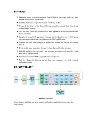
The document describes a study that used a convolutional neural network with a ConvNeXtLarge architecture to classify skin cancer images into benign and malignant classes. The CNN model was trained on a dataset of 3,297 skin cancer images from Kaggle. It achieved an AUC of 0.91 for classifying the images, demonstrating the ConvNeXtLarge architecture is effective for this task. The study aims to help early diagnosis and treatment of skin cancers.

![Relevant Literature :
Author Feature/methods Performance
Abhinav Sagar,
Dheeba Jacob [12]
CNN (ResNet50,
DenseNet,169,InceptionV3,
MobileNet ,InceptionResNet v2)
Accuracy: 93.5%
AUC – 86.1%
Taki Hasan Rafi
Mehadi Hassan [13]
CNN (VGG19,
ResNet50,EfficientNetB0)
Training Accuracy: 98.67%
Precision: 91.6%
Recall: 92.88%
F1-Score: 91.27%
Ali, Karar, et al. [2] CNN (EfficientNets B4) Accuracy: 87.1%
F1-Score: 87%
Hekler, Achim, et al. [3] CNN Accuracy: 82.95%
Sensitivity: 89%
Specificity: 84%
Hosny, Khalid M., Mohamed
A. Kassem, and Mohamed M.
Foaud. [4]
CNN(AlexNet) Sensitivity: 86.26%
Specificity: 98.93%
Accuracy: 98.61%
Precision: 97.73%
Chaturvedi, Saket S., Jitendra
V. Tembhurne, and Tausif
Diwan. [5]
CNN (ResNeXt101) Accuracy: 92.83%
Dubal, Pratik, et al. [11] Neural Network Accuracy: 76.9%
Ali, Md Shahin, et al. [7] DCNN (AlexNet, ResNet, VGG-
16, DenseNet, MobileNet)
Accuracy: 91.93%
Javaid, Arslan, Muhammad
Sadiq, and Faraz Akram. [10]
ML (Random Forest) + Image
Processing
Accuracy: 93.89%
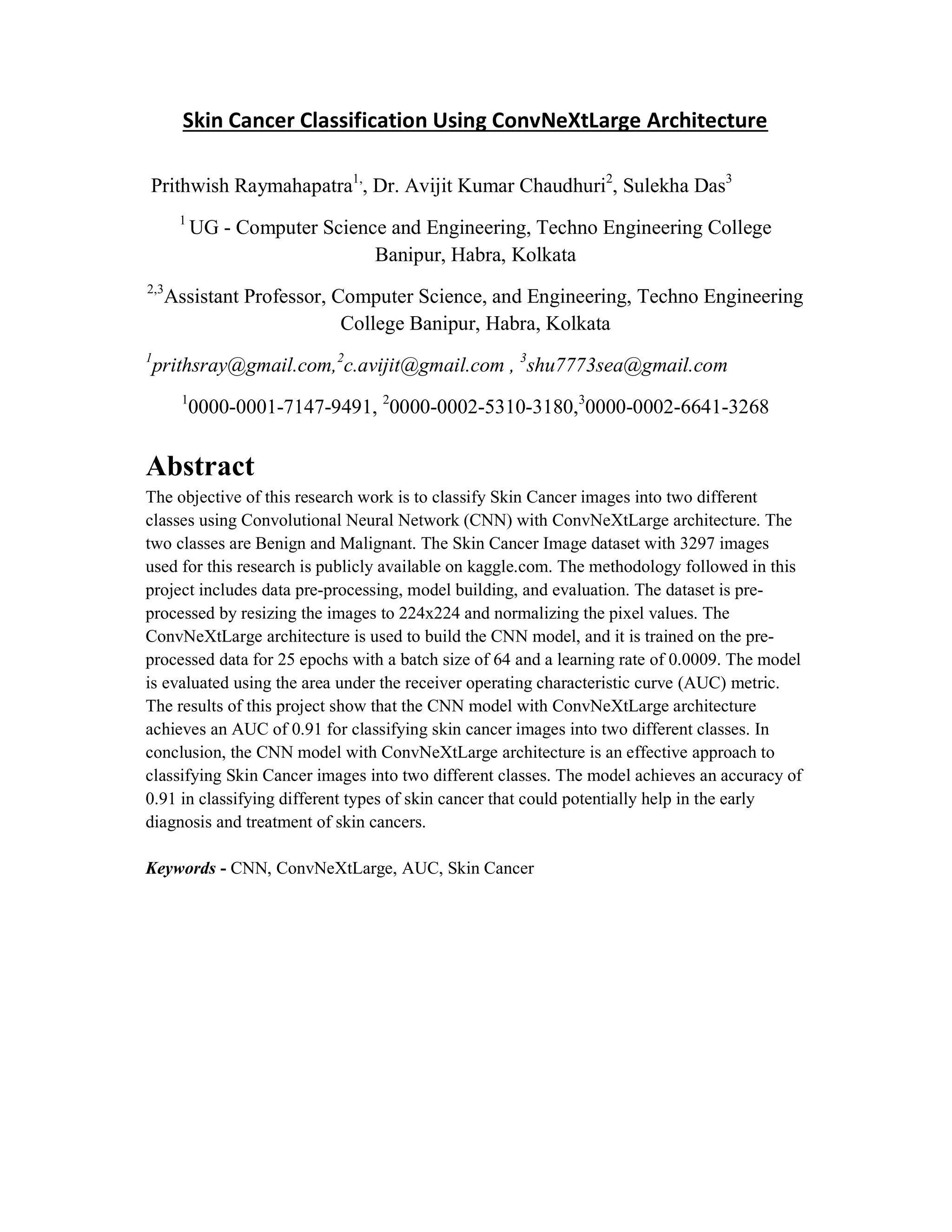
Table 1: Literature Study
Table 1 shows the literature review of various skin cancer research work](https://image.slidesharecdn.com/researchpaper2023skincancer-240327021022-8f6f5908/85/researchpaper_2023_Skin_Csdbjsjvnvsdnfvancer-pdf-3-320.jpg)
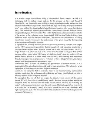
![Methodology:
Dataset: The first step of this whole research work was selecting the dataset. In this
case, we have chosen a dataset which is a processed Skin Cancer picture of the ISIC
Archive. This dataset contains 3297 images of human skin cancer disease, classified
into 2 classes: benign and malignant. The particular reason behind working with this
dataset is that this dataset consists of a lot of sample images and a lot of research work
has already been done with this dataset and got remarkable results. The dataset was
divided into two parts: the training set and the testing set. The training set contains a
total of 2637 images and the testing set consists of 660 images. Each of the two
consists of all the 2 classes i.e. benign and malignant.
Training Set Testing Set
benign 1440 360
meningioma 1197 300
Table 2: Train Test Divisions
Table 2 shows the Training and testing division of the data that have been used in this article
Research Method:
Convolutional Neural Network: CNN[23] stands for Convolutional Neural
Network, which is a type of deep neural network i.e. deep learning commonly used in
image and video recognition and also to process any tasks. The key characteristic of
CNN is that it can automatically learn and extract features from the raw data, in this
case, images or videos. These features are learned through a process of convolution,
where the network applies a complete set of filters or kernels to the input image to
identify patterns and structures in the data. The output of the convolutional layers is
then passed through a series of pooling layers, which reduce the spatial size of the
features and help to increase the network's ability to generalize to new images. After
the pooling layers, the resulting features are flattened into a vector and fed into the
fully connected layer, where the network can make predictions based on the learned
features. CNNs have proven to be highly effective in a range of computer vision tasks,
including classification of the image, the detection of objects, and segmentation.](https://image.slidesharecdn.com/researchpaper2023skincancer-240327021022-8f6f5908/85/researchpaper_2023_Skin_Csdbjsjvnvsdnfvancer-pdf-4-320.jpg)
![ ConvNeXtLarge: ConvNeXtLarge[24] is a variant of the ConvNeXt
architecture that is designed to be larger and more complex. ConvNeXt is a
convolutional neural network (CNN) architecture that aims to improve the
accuracy of image classification models while reducing the number of
parameters needed. The ConvNeXt architecture combines grouped
convolutions and concatenation of the output of these grouped convolutions in
parallel. Grouped convolution is a technique that divides the input feature maps
into several groups and applies a convolutional layer on each group
independently. By doing so, it reduces the number of parameters in the network
and improves the efficiency of the computation. The "ConvNeXtLarge" might
refer to a specific variant of the ConvNeXt architecture that is particularly large
and complex, possibly with more layers or neurons than other variants.
Figure 1: ConvNeXt Architecture
Figure 1 shows the ConvNeXt Architecture that has been used in this article
Resnet50: ResNet50[12] is a variant of the Residual Neural Network (ResNet)
architecture. It is a deep CNN architecture that has achieved state-of-the-art
performance on several image classification datasets, including ImageNet. ResNet50
consists of 50 layers, including convolutional layers, pooling layers, fully connected
layers, and skip connections. The skip connections are the key innovation of the
ResNet architecture, and they help to address the problem of vanishing gradients that
can occur in deep networks. The skip connections enable the network to learn residual
functions, which are the difference between the input and the output of a block of
layers. By doing so, the network can more easily learn identity mapping, which is a
key component of the residual function.](https://image.slidesharecdn.com/researchpaper2023skincancer-240327021022-8f6f5908/85/researchpaper_2023_Skin_Csdbjsjvnvsdnfvancer-pdf-5-320.jpg)
![Figure 2: ResNet Architecture
Figure 2 shows the ResNet Architecture that has been used in this article
DenseNet201: DenseNet201 is a variant of the DenseNet architecture. DenseNet201
is a deep convolutional neural network (CNN) architecture that has achieved state-of-
the-art performance on several benchmark image classification datasets, including
ImageNet.The DenseNet architecture is based on the idea of dense connections
between layers, where each layer receives the feature maps of all preceding layers as
input. By doing so, the network can make better use of the features learned by the
earlier layers and improve the flow of information through the network.
Figure 3: DenseNet Architecture
Figure 3 shows the DenseNet Architecture that has been used in this article
ImageNet: The ImageNet [22] weights for ConvNeXtLarge are pre-trained weights
that have been learned on the large-scale ImageNet dataset. These weights are often
used as starting point for transfer learning in computer vision tasks This includes the
weights for all the layers in the network, as well as the biases for the fully connected
layers.](https://image.slidesharecdn.com/researchpaper2023skincancer-240327021022-8f6f5908/85/researchpaper_2023_Skin_Csdbjsjvnvsdnfvancer-pdf-6-320.jpg)
![ ImageDataGenerator: In Keras, the ImageDataGenerator[21] class is used for image
generation and data augmentation. This class provides a set of functions for pre-
processing and data augmentation on the input images. It generates batches of tensor
image data using real-time data augmentation. This allows you to train deep learning
models on a large dataset without having to load all the images into memory at once.
Instead, the ImageDataGenerator loads the images in batches and applies various
image transformations on the fly.
PRIMARY WORK: The first step of this whole research work was selecting the dataset.
In this case, we have chosen a dataset which is a processed Skin Cancer picture of the ISIC
Archive. This dataset contains 3297 images of human skin cancer disease, classified into 2
classes: Benign and Malignant. The particular reason behind working with this dataset is that
this dataset has a lot of sample images and a lot of research work has already been done with
this dataset and got remarkable results.
After the selection of the dataset, we used the ConvNeXtLarge model that came out in 2020
which is one of the latest CNN models available right now and haven’t been used in many
classification models, but due to its unique architecture, we have got the best results in this
model over DenseNet, Resnet50 which are less discriminative.
Post training the model over the dataset, we tested it over the testing set and got remarkable
results with the classifications. The various parameters of measuring the performance i.e.
accuracy, recall, precision, specificity, F1-score, and AUC of this research are depicted later.
Confusion Matrix: A confusion matrix [20] i.e. also called an error matrix, is one type of
matrix or a table where we put the results of the MLR model i.e. the test data. The confusion
matrix is the shortest way to see and understand the result of the model. In the confusion
matrix, there are a total of four variables as – TP, TN, FP, and FN. TP stands for 'true
positive' which shows the total number of positive data classified accurately. TN stands for
'true negative' which shows the total number of negative data classified accurately. FP stands
for 'false positive' which indicates the real value is negative but predicted as positive. FP is
called a TYPE 1 ERROR. FN stands for 'false negative' which indicates the real value is
positive but predicted as negative. FN is also called a TYPE 2 ERROR.](https://image.slidesharecdn.com/researchpaper2023skincancer-240327021022-8f6f5908/85/researchpaper_2023_Skin_Csdbjsjvnvsdnfvancer-pdf-7-320.jpg)
![TP
Recall =
TP+FN
Recall is calculated as the
ratio of the number of positive samples
correctly classified as positive to the total
number of positive samples. Recall measures
the ability of a model to detect positive
samples. The higher the recall, the more
positive samples are found.
FP
FPR
TN FP
It is the probability of falsely rejecting the
null hypothesis.
2 * Recall * Precision
F1_Score =
Recall + Precision
F1 score is the measurement of accuracy and
it is the harmonic mean of precision and
recall. Its maximum value can be 1 and the
minimum value can be 0.
1 FPR recall
auc= - +
2 2 2
AUC [14] stands for Area Under the ROC
Curve, which is a popular evaluation metric
in machine learning for binary classification
problems. The ROC (Receiver Operating
Characteristic) curve is a graphical
representation of the performance of a binary
classifier, and the AOC measures the area
under this curve. In a problem that is binary
classified, the classifier tries to predict
whether an input belongs to a positive or
negative class. The ROC curve plots the true
positive rate (TPR) against the false positive
rate (FPR) for different classification
thresholds. The TPR is the ratio of correctly
predicted positive samples to the total
number of actual positive samples, and the
FPR is the ratio of incorrectly predicted
positive samples to the total number of actual
negative samples. The AOC ranges from 0 to
1, with higher values indicating better
performance. A perfect classifier would have
an AOC of 1, while a completely random
classifier would have an AOC of 0.5. The
AOC is a useful evaluation metric because it
takes into account all possible classification
thresholds and provides a single number to
compare the performance of different
classifiers.](https://image.slidesharecdn.com/researchpaper2023skincancer-240327021022-8f6f5908/85/researchpaper_2023_Skin_Csdbjsjvnvsdnfvancer-pdf-9-320.jpg)
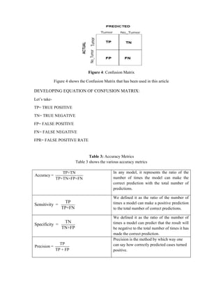
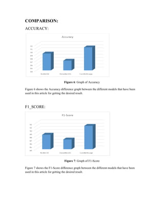
![RESULTS AND DISCUSSION
After analyzing the ConvNeXtLarge model and other CNN models like ResNet50, and
DenseNet on this dataset we get the results that are given below.
Model Accuracy
(%)
Precision
(%)
Recall
(%)
AUC
(%)
F1-Score
(%)
ResNet50 89.24 90.66 86.34 89.11 88.45
DenseNet201 87.03 86.56 87.38 87.03 86.97
ConvNeXtLarge 91.17 91.25 91.10 91.17 91.17
Table 4: Comparisons Table
Table 4 shows the Comparison of different metrics from different models that have been used
to get the desired results.
ConvNeXtLarge[24] is a variant of the ConvNeXt architecture that is designed to be
larger and more complex. ConvNeXt is a convolutional neural network (CNN)
architecture which is a modified version of ResNet architecture that uses the Vision
Transformers(VIT) technology and aims to improve the accuracy of image
classification models while reducing the number of parameters needed, these
Convolution Nets with this vision transformer technology make up a powerful neural
network but instead of its wide scalability these VIT had some shortcomings due to
higher resolution of inputs, to solve these problems the sliding window approach was
again reintroduced in Swin Transformers which made it a first transformer to act as a
generic vision backbone and to aid in image classification tasks. Unlike the ResNet
style stem cell, the ConvNeXt architecture uses the patchify layer that is used by Swin
transformers and combines grouped convolutions and concatenation of the output of
these grouped convolutions in parallel. Grouped convolution is a technique that
divides the input feature maps into several groups and applies a convolutional layer on
each group independently. By doing so, it reduces the number of parameters in the
network and improves the efficiency of the computation. The "ConvNeXtLarge"
might refer to a specific variant of the ConvNeXt architecture that is particularly large
and complex, possibly with more layers or neurons than other variants.](https://image.slidesharecdn.com/researchpaper2023skincancer-240327021022-8f6f5908/85/researchpaper_2023_Skin_Csdbjsjvnvsdnfvancer-pdf-11-320.jpg)
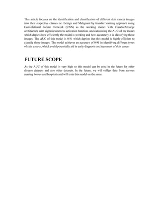
![AUC:
Figure 8 shows the AUC difference graph
in this article for getting the desired result.
CONCLUSION
Author
Abhinav Sagar,
Dheeba Jacob [12]
CNN (ResNet50,
DenseNet,169,InceptionV3,
MobileNet ,InceptionResNet v2)
Taki Hasan Rafi
Mehadi Hassan [13]
CNN (VGG19,
ResNet50,EfficientNetB0)
Proposed architecture CNN( ConvNeXtLarge )
Table 5: ISIC Skin Cancer Dataset Performance Comparison
Table 5 shows the comparative study of different metrics used in the same dataset.
Figure 8: Graph of AUC
shows the AUC difference graph between the different models that have been used
in this article for getting the desired result.
Feature/methods Performance
CNN (ResNet50,
DenseNet,169,InceptionV3,
MobileNet ,InceptionResNet v2)
Accuracy: 93.5%
AUC – 86.1%
CNN (VGG19,
ResNet50,EfficientNetB0)
Training Accuracy: 98.67%
Precision: 91.6%
Recall: 92.88%
F1-Score: 91.27%
CNN( ConvNeXtLarge ) Accuracy: 91.17 %
Precision: 91.25 %
Recall: 91.10 %
F1-Score: 91.17 %
AUC: 91.17 %
ISIC Skin Cancer Dataset Performance Comparison
Table 5 shows the comparative study of different metrics used in the same dataset.
between the different models that have been used
Performance
%
Training Accuracy: 98.67%
%
%
91.17 %
91.25 %
91.17 %
Table 5 shows the comparative study of different metrics used in the same dataset.](https://image.slidesharecdn.com/researchpaper2023skincancer-240327021022-8f6f5908/85/researchpaper_2023_Skin_Csdbjsjvnvsdnfvancer-pdf-13-320.jpg)
![REFERENCES:
[1] https://www.kaggle.com/datasets/fanconic/skin-cancer-malignant-vs-benign/
[2] Ali, K., Shaikh, Z. A., Khan, A. A., & Laghari, A. A. (2022). Multiclass skin cancer
classification using EfficientNets–a first step towards preventing skin cancer. Neuroscience
Informatics, 2(4), 100034.
[3] Hekler, A., Utikal, J. S., Enk, A. H., Hauschild, A., Weichenthal, M., Maron, R. C., ... &
Thiem, A. (2019). Superior skin cancer classification by the combination of human and
artificial intelligence. European Journal of Cancer, 120, 114-121.
[4] Hosny, K. M., Kassem, M. A., & Foaud, M. M. (2018, December). Skin cancer
classification using deep learning and transfer learning. In 2018 9th Cairo international
biomedical engineering conference (CIBEC) (pp. 90-93). IEEE.
[5] Chaturvedi, S. S., Tembhurne, J. V., & Diwan, T. (2020). A multi-class skin Cancer
classification using deep convolutional neural networks. Multimedia Tools and Applications,
79(39-40), 28477-28498.
[6] Höhn, J., Hekler, A., Krieghoff-Henning, E., Kather, J. N., Utikal, J. S., Meier, F., ... &
Brinker, T. J. (2021). Integrating patient data into skin cancer classification using
convolutional neural networks: systematic review. Journal of Medical Internet Research,
23(7), e20708.
[7] Ali, M. S., Miah, M. S., Haque, J., Rahman, M. M., & Islam, M. K. (2021). An enhanced
technique of skin cancer classification using a deep convolutional neural network with
transfer learning models. Machine Learning with Applications, 5, 100036.
[8] Elgamal, M. (2013). Automatic skin cancer image classification. International Journal of
Advanced Computer Science and Applications, 4(3).
[9] Fu’adah, Y. N., Pratiwi, N. C., Pramudito, M. A., & Ibrahim, N. (2020, December).
Convolutional neural network (CNN) for automatic skin cancer classification system. In IOP
conference series: materials science and engineering (Vol. 982, No. 1, p. 012005). IOP
Publishing.
[10] Javaid, A., Sadiq, M., & Akram, F. (2021, January). Skin cancer classification using
image processing and machine learning. In 2021 International Bhurban conference on applied
sciences and Technologies (IBCAST) (pp. 439-444). IEEE.
[11] Dubal, P., Bhatt, S., Joglekar, C., & Patil, S. (2017, November). Skin cancer detection
and classification. In 2017 6th international conference on electrical engineering and
Informatics (ICEEI) (pp. 1-6). IEEE.
[12] Sagar, A., & Dheeba, J. (2020). Convolutional neural networks for classifying melanoma
images. bioRxiv, 2020-05.](https://image.slidesharecdn.com/researchpaper2023skincancer-240327021022-8f6f5908/85/researchpaper_2023_Skin_Csdbjsjvnvsdnfvancer-pdf-15-320.jpg)
![[13] Rafi, T. H., & Hassan, M. (2020). Efficient classification of benign and malignant
tumors implementing various deep convolutional neural networks. Int J Comput Sci Eng
Appl, 9(2), 152-158.
[14] Pal, S. S., Raymahapatra, P., Paul, S., Dolui, S., Chaudhuri, A. K., & Das, S. A Novel
Brain Tumor Classification Model Using Machine Learning Techniques.
[15] Saha, S., Mondal, J., Arnam Ghosh, M., Das, S., & Chaudhuri, A. K. Prediction on the
Combine Effect of Population, Education, and Unemployment on Criminal Activity Using
Machine Learning.
[16] Dey, R., Bose, S., Ghosh, N., Chakraborty, S., Kumar, A., & Chaudhuri, S. D. An
Extensive Review on Cancer Detection using Machine Learning Algorithms.
[17] Ray, A., & Chaudhuri, A. K. (2021). Smart healthcare disease diagnosis and patient
management: Innovation, improvement and skill development. Machine Learning with
Applications, 3, 100011.
[18] Chaudhuri, A. K., Banerjee, D. K., & Das, A. (2021). A Dataset Centric Feature
Selection and Stacked Model to Detect Breast Cancer. International Journal of Intelligent
Systems and Applications (IJISA), 13(4), 24-37.
[19] Chaudhuri, A. K., Ray, A., Banerjee, D. K., & Das, A. (2021). An Enhanced Random
Forest Model for Detecting Effects on Organs after Recovering from Dengue. methods, 8(8).
[20] Pal, S. S., Paul, S., Dey, R., Das, S., & Chaudhuri, A. K. Determining the probability of
poverty levels of the Indigenous Americans and Black Americans in the US using Multiple
Regression.
[21] Shorten, C., & Khoshgoftaar, T. M. (2019). A survey on image data augmentation for
deep learning. Journal of big data, 6(1), 1-48.
[22] Krizhevsky, A., Sutskever, I., & Hinton, G. E. (2017). Imagenet classification with deep
convolutional neural networks. Communications of the ACM, 60(6), 84-90.
[23] Girshick, R. (2015). Fast r-CNN. In Proceedings of the IEEE international conference on
computer vision (pp. 1440-1448).
[24] Pham, L., Le, C., Ngo, D., Nguyen, A., Lampert, J., Schindler, A., & McLoughlin, I.
(2023). A Light-weight Deep Learning Model for Remote Sensing Image Classification.
arXiv preprint arXiv:2302.13028.](https://image.slidesharecdn.com/researchpaper2023skincancer-240327021022-8f6f5908/85/researchpaper_2023_Skin_Csdbjsjvnvsdnfvancer-pdf-16-320.jpg)