The document provides an introduction to numerical methods, focusing on their application in solving complex engineering problems where analytical methods fall short. It describes the process of solving equations through iterative approximations, emphasizes the significance of accuracy and precision in computations, and discusses types of errors, including truncation and round-off errors. Additionally, it covers methods for measuring errors, estimation improvements, and includes examples related to Taylor series and Maclaurin series expansions.

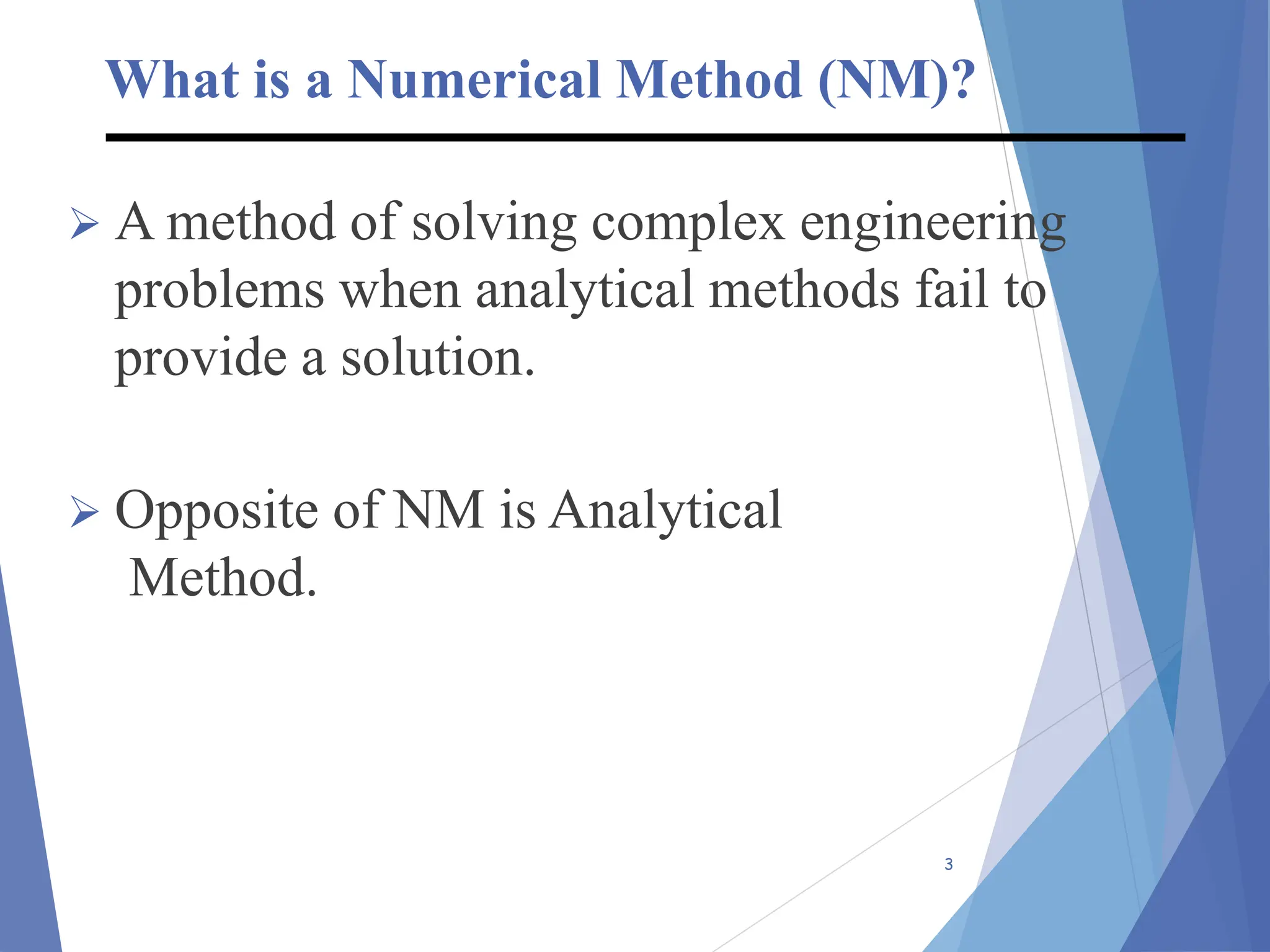
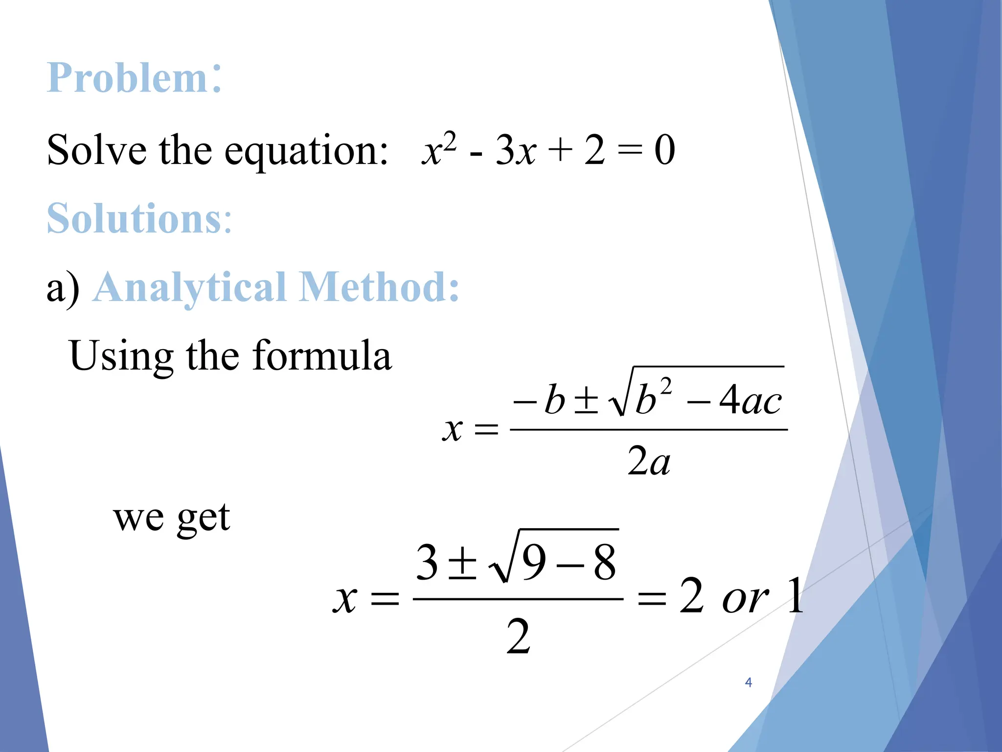
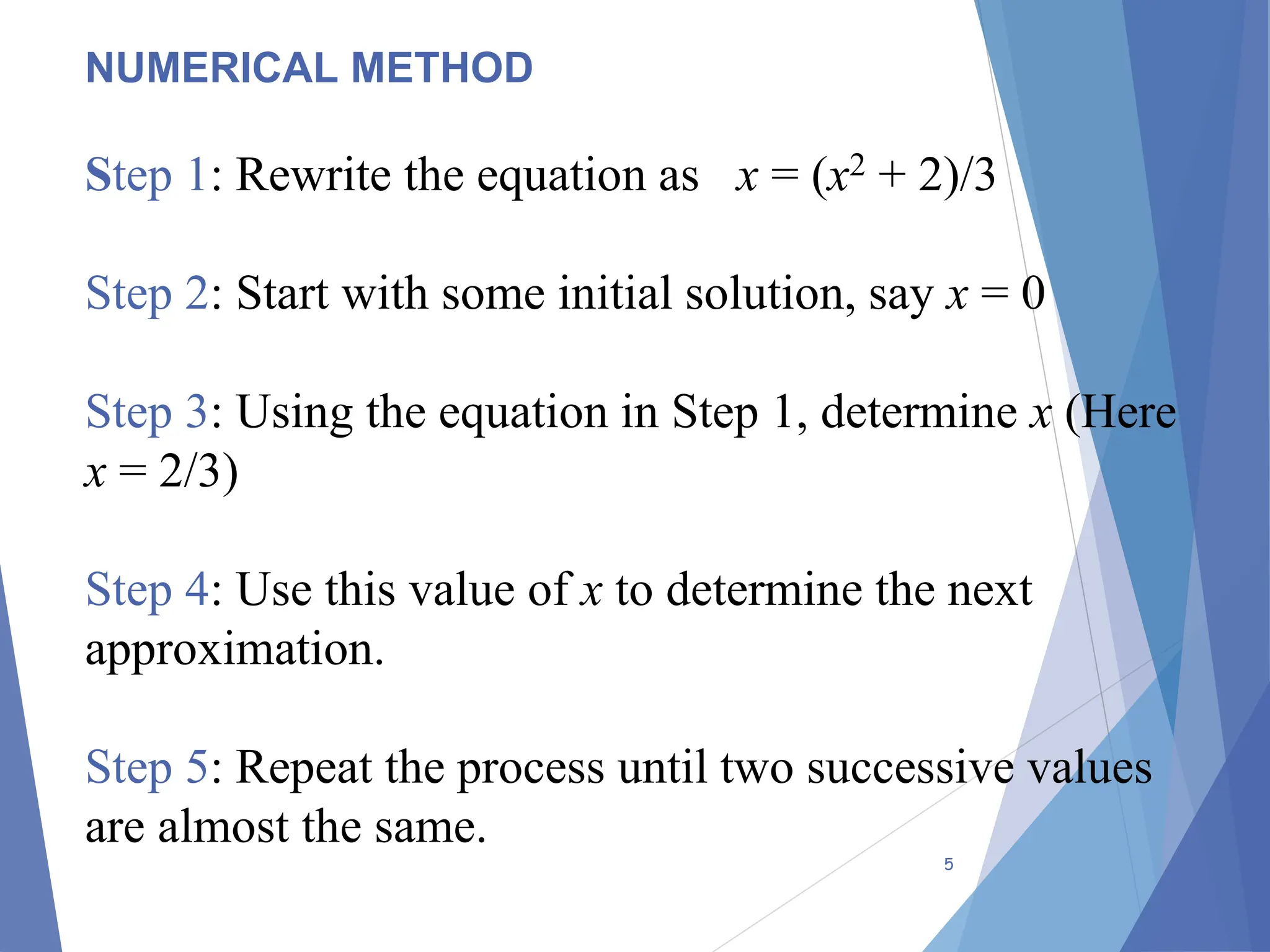
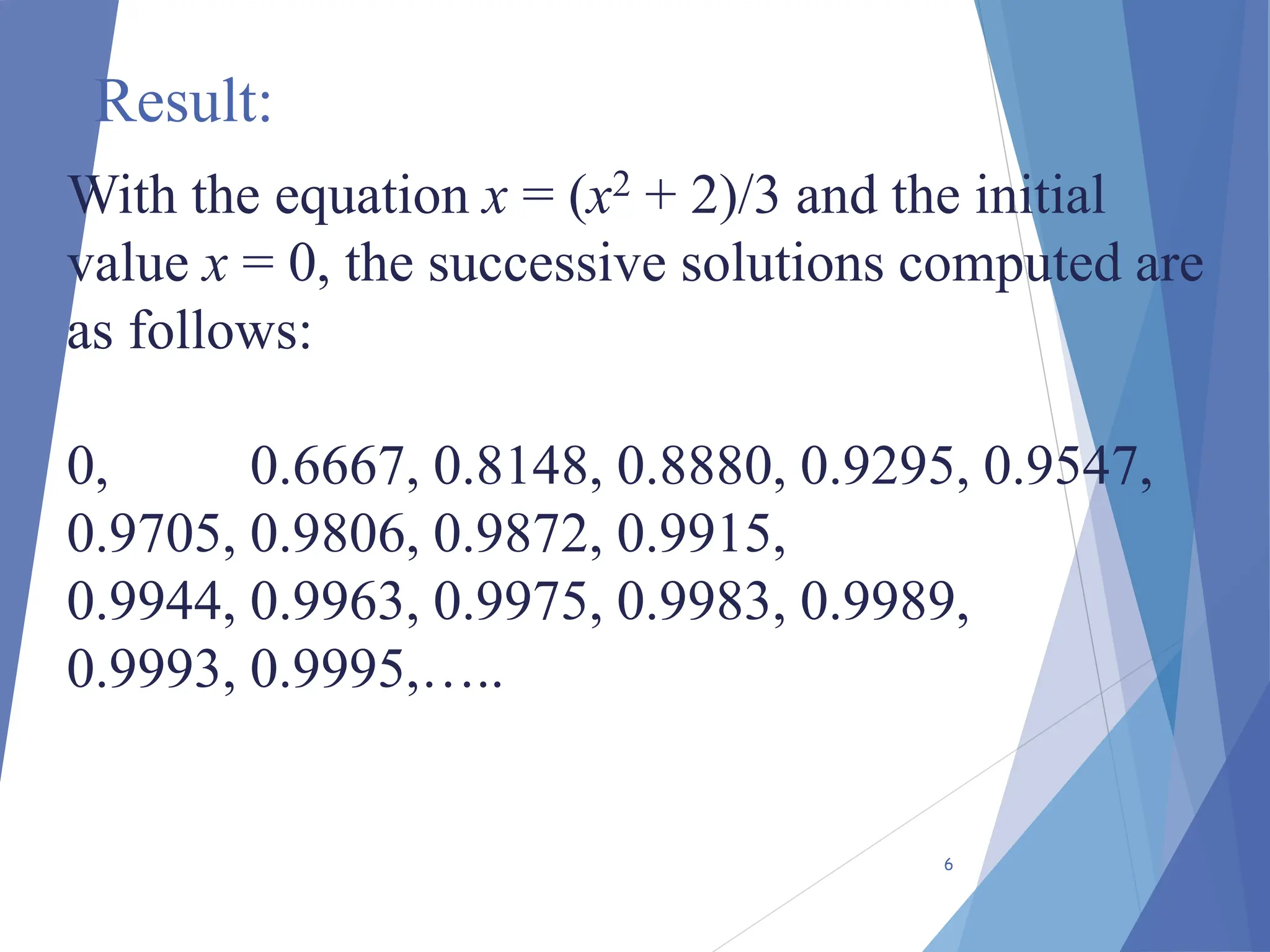
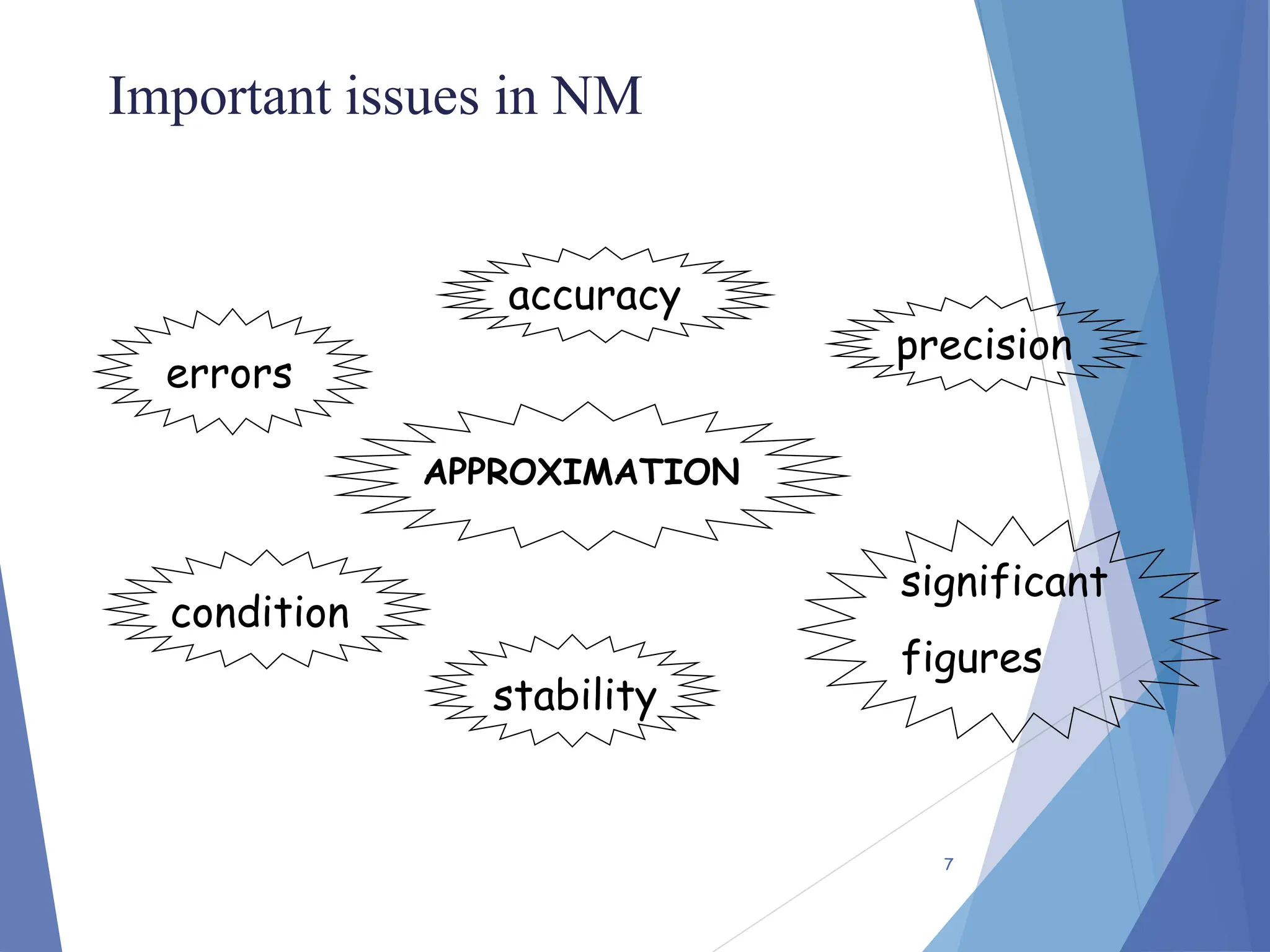
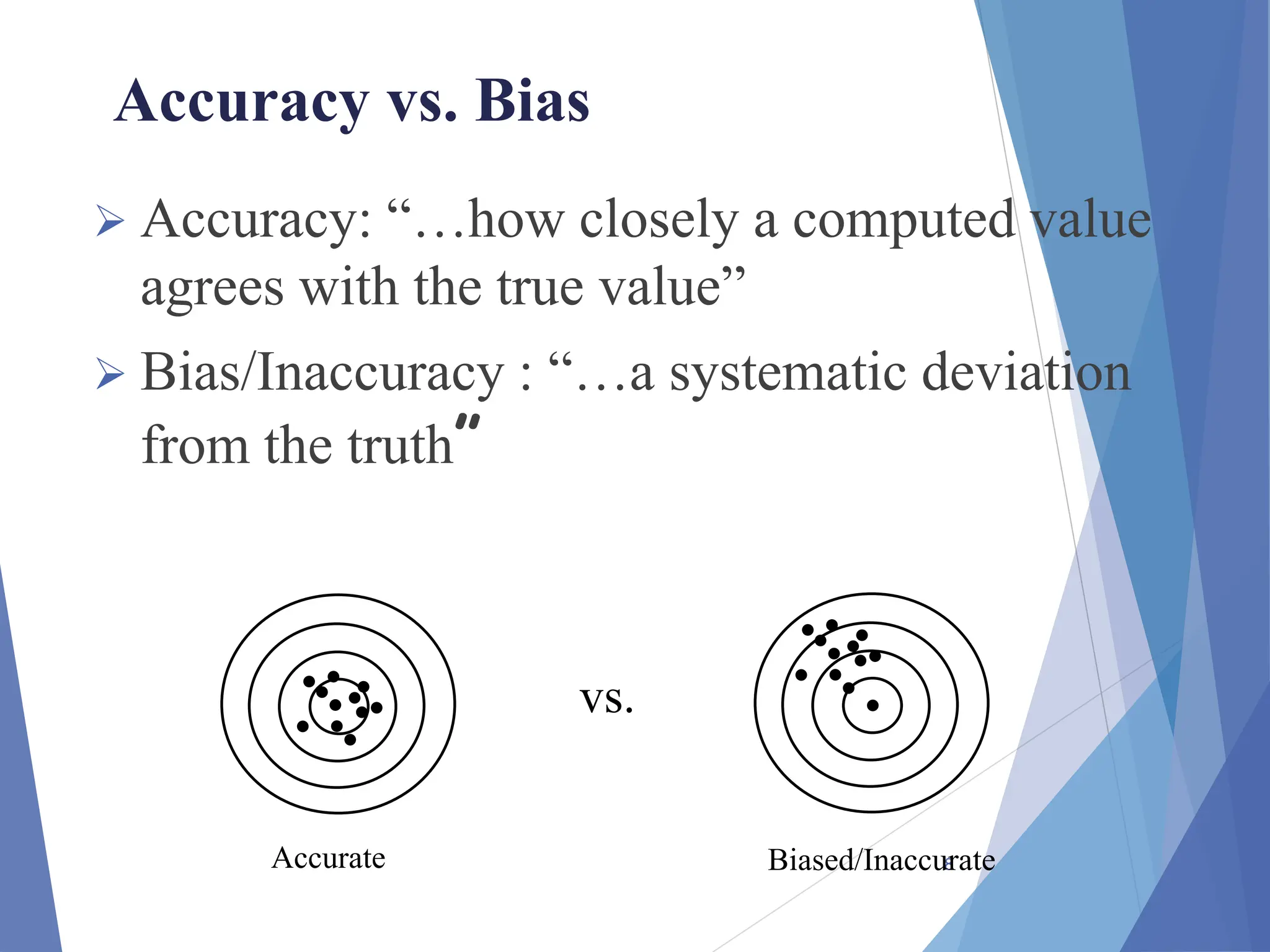
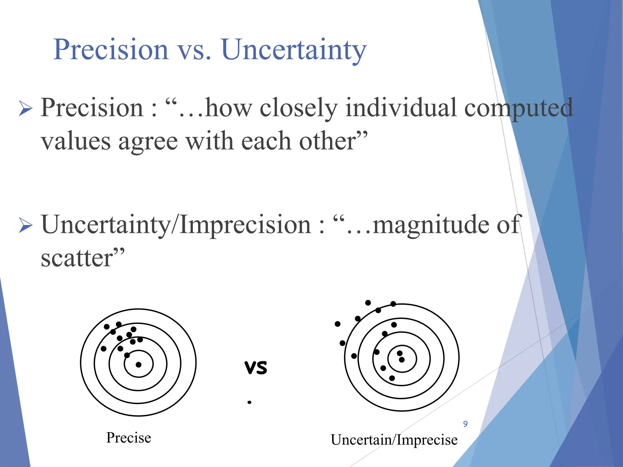
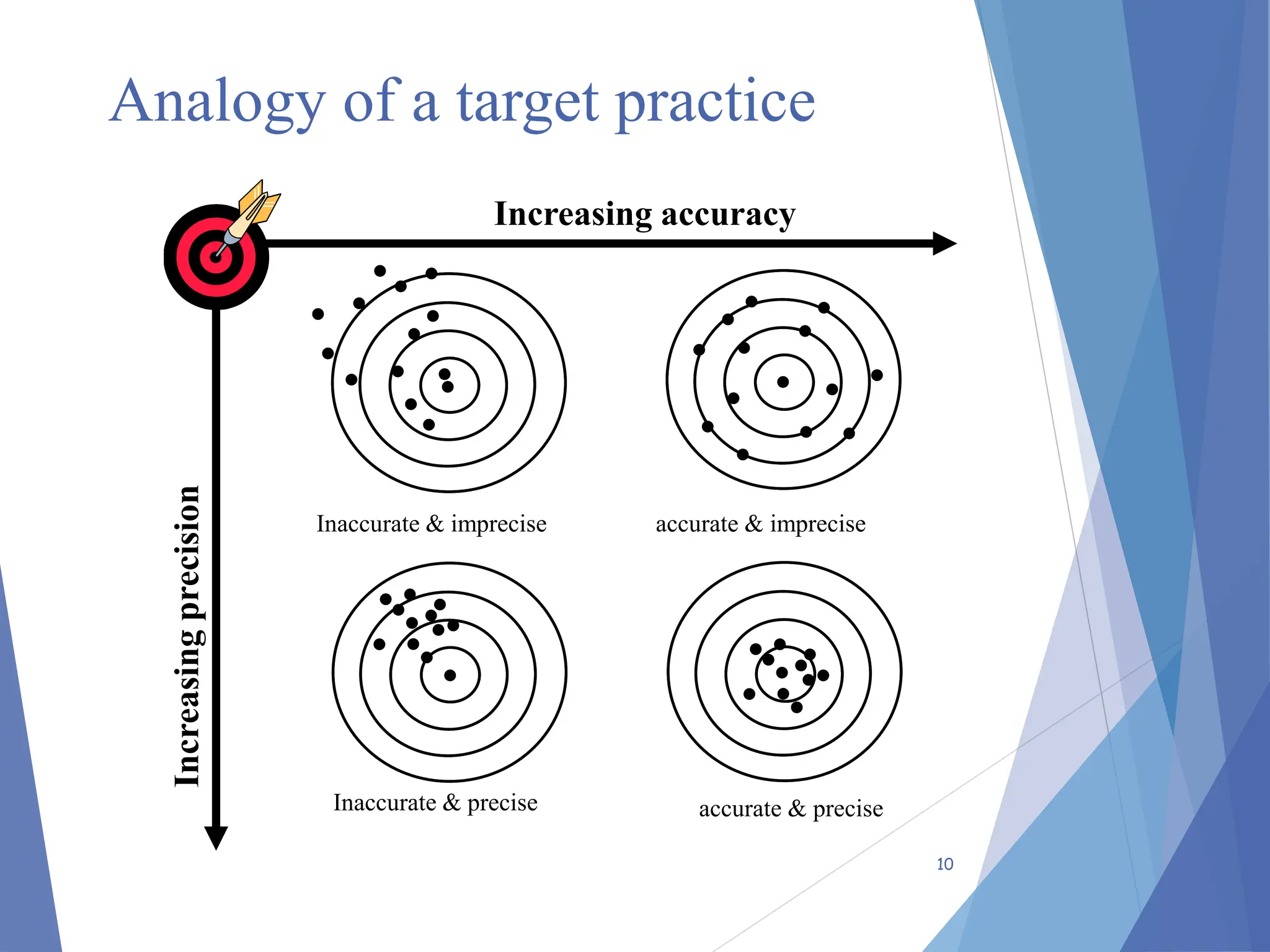
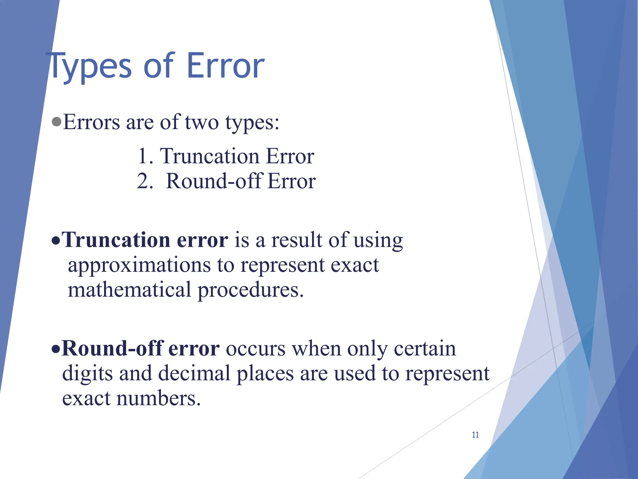
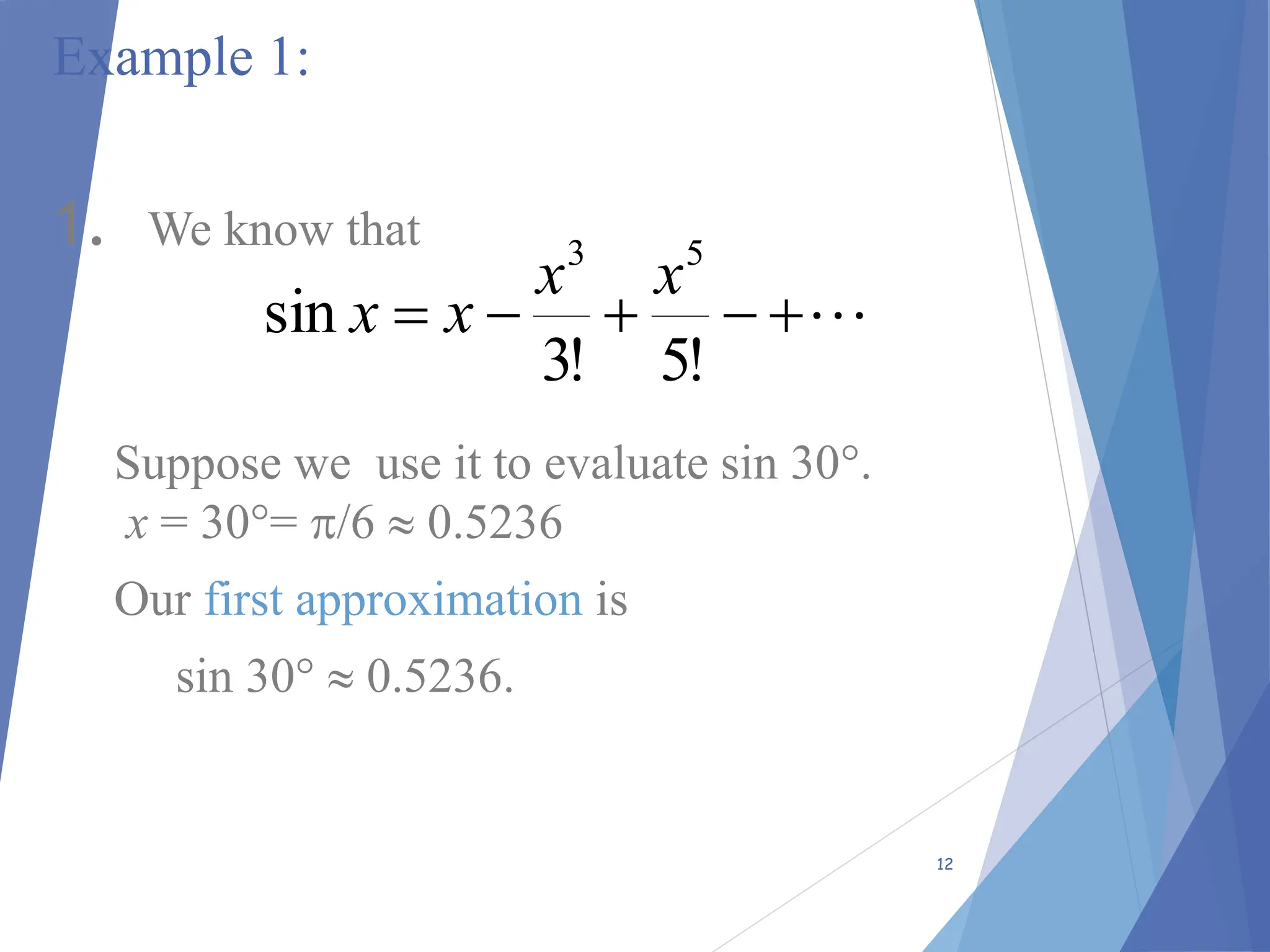
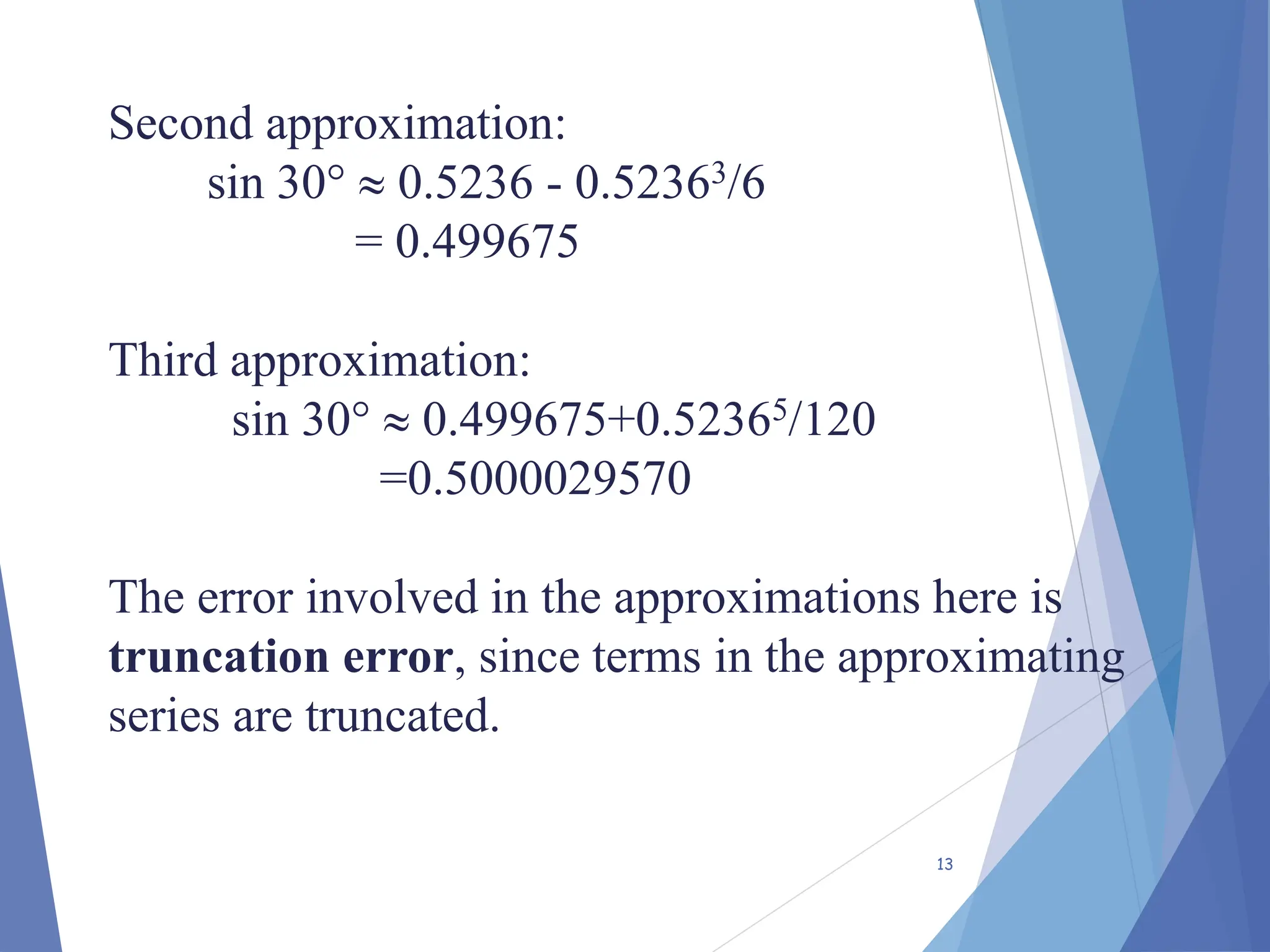
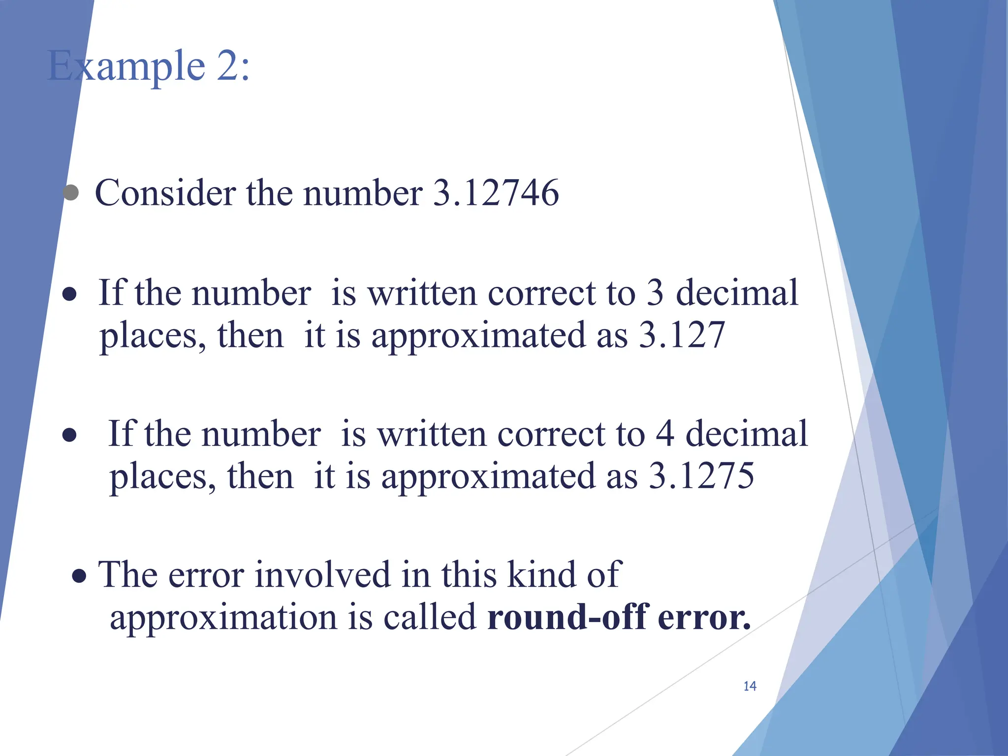
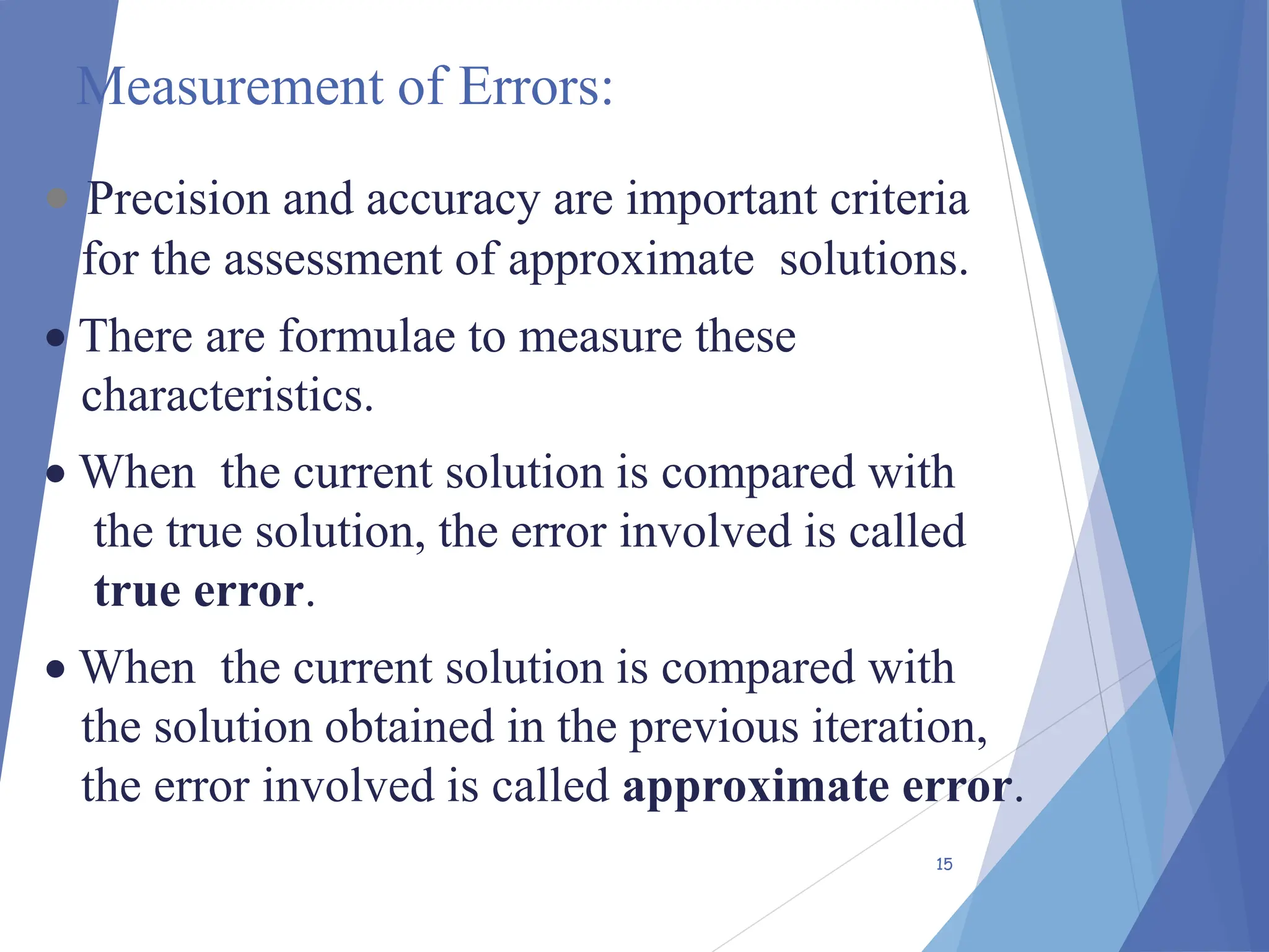
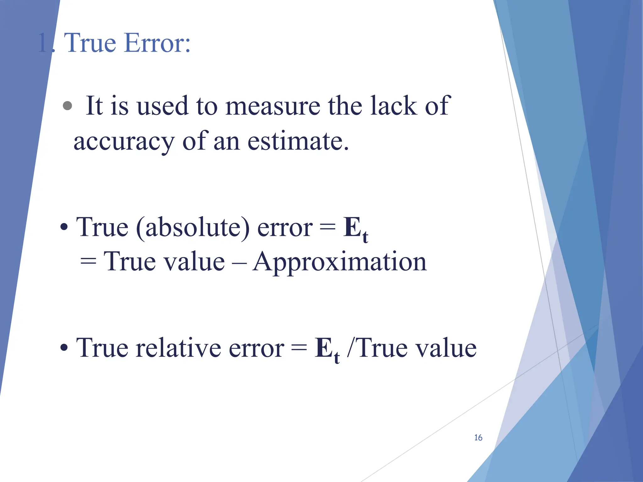
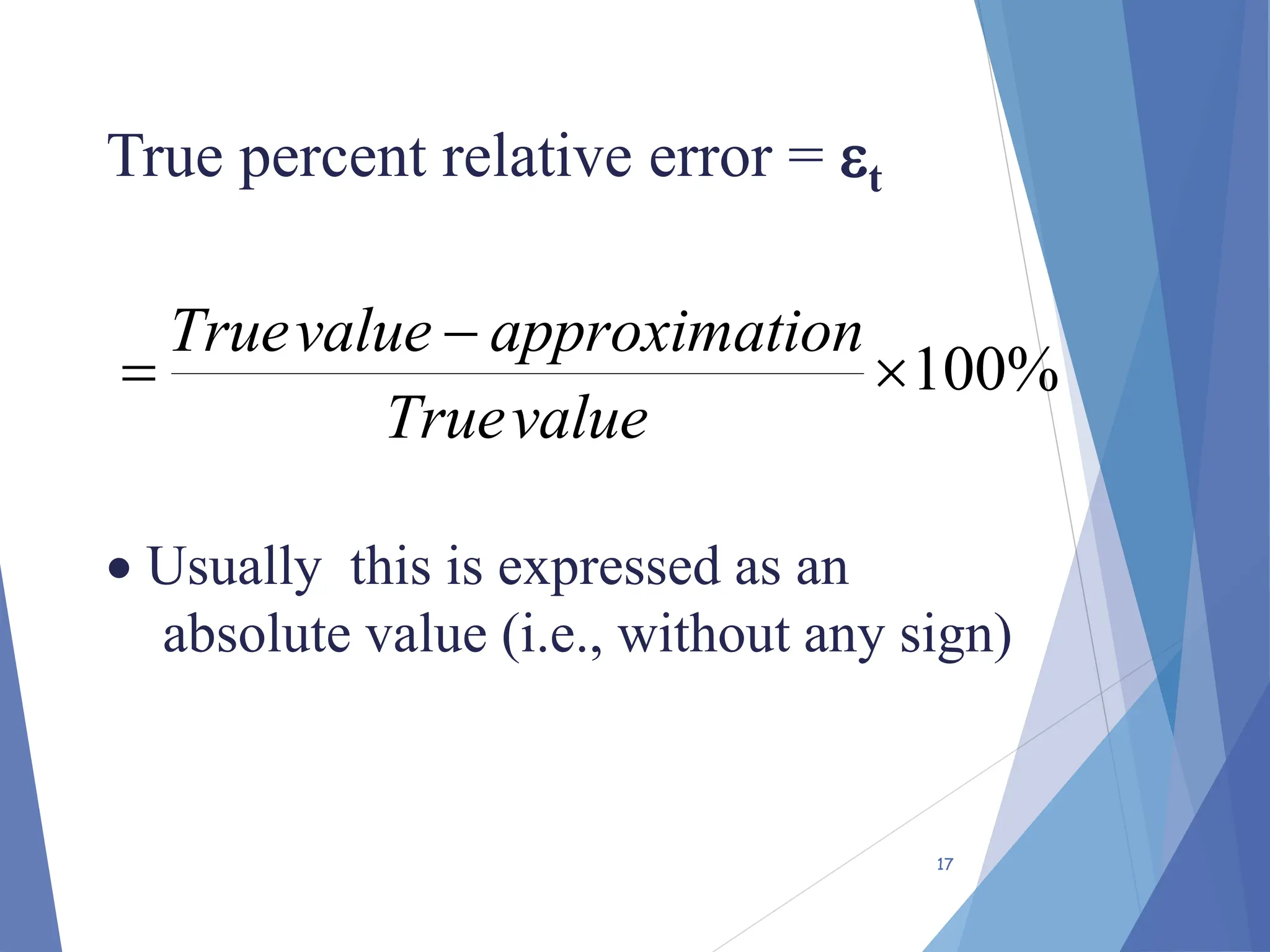
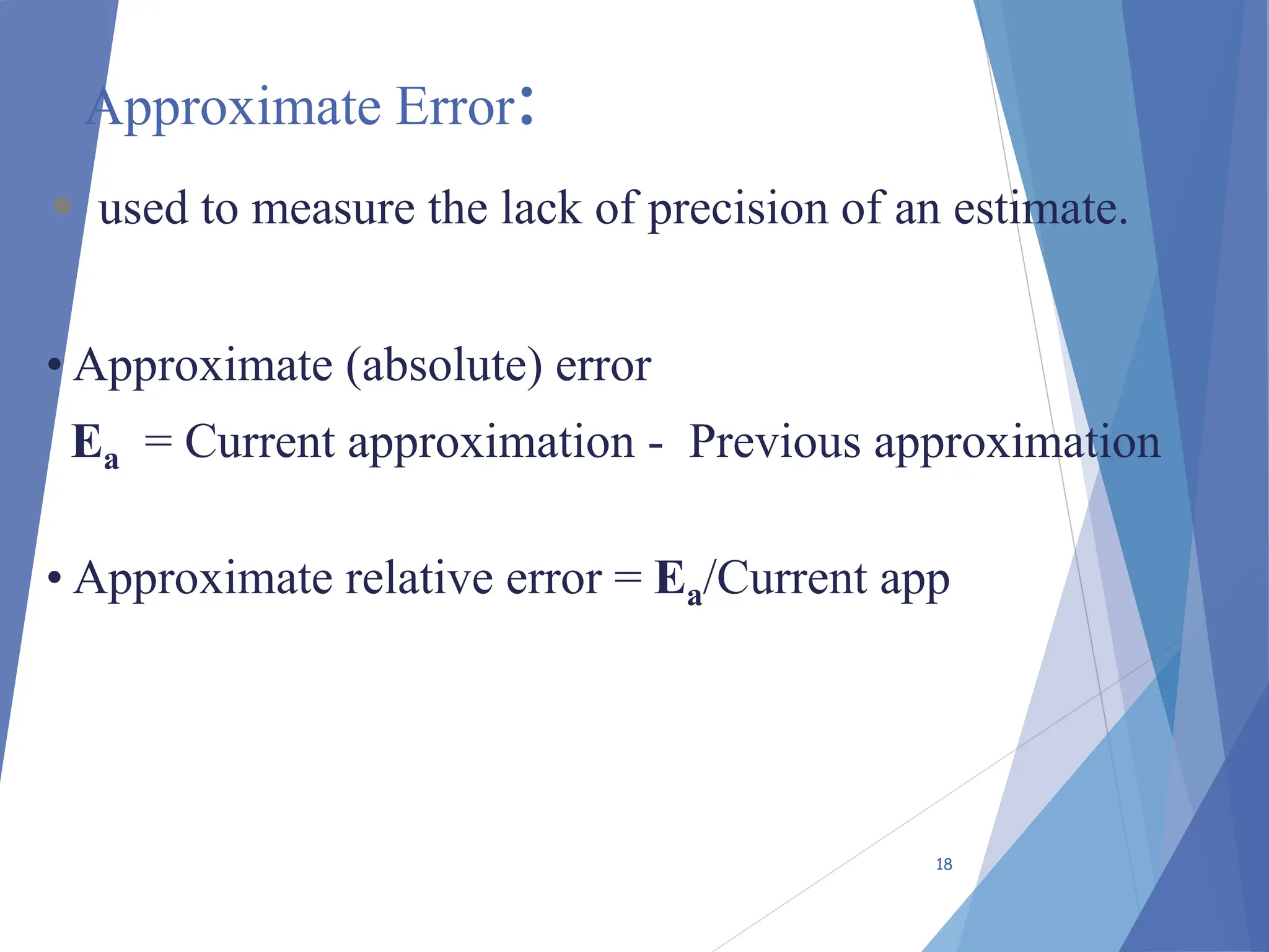
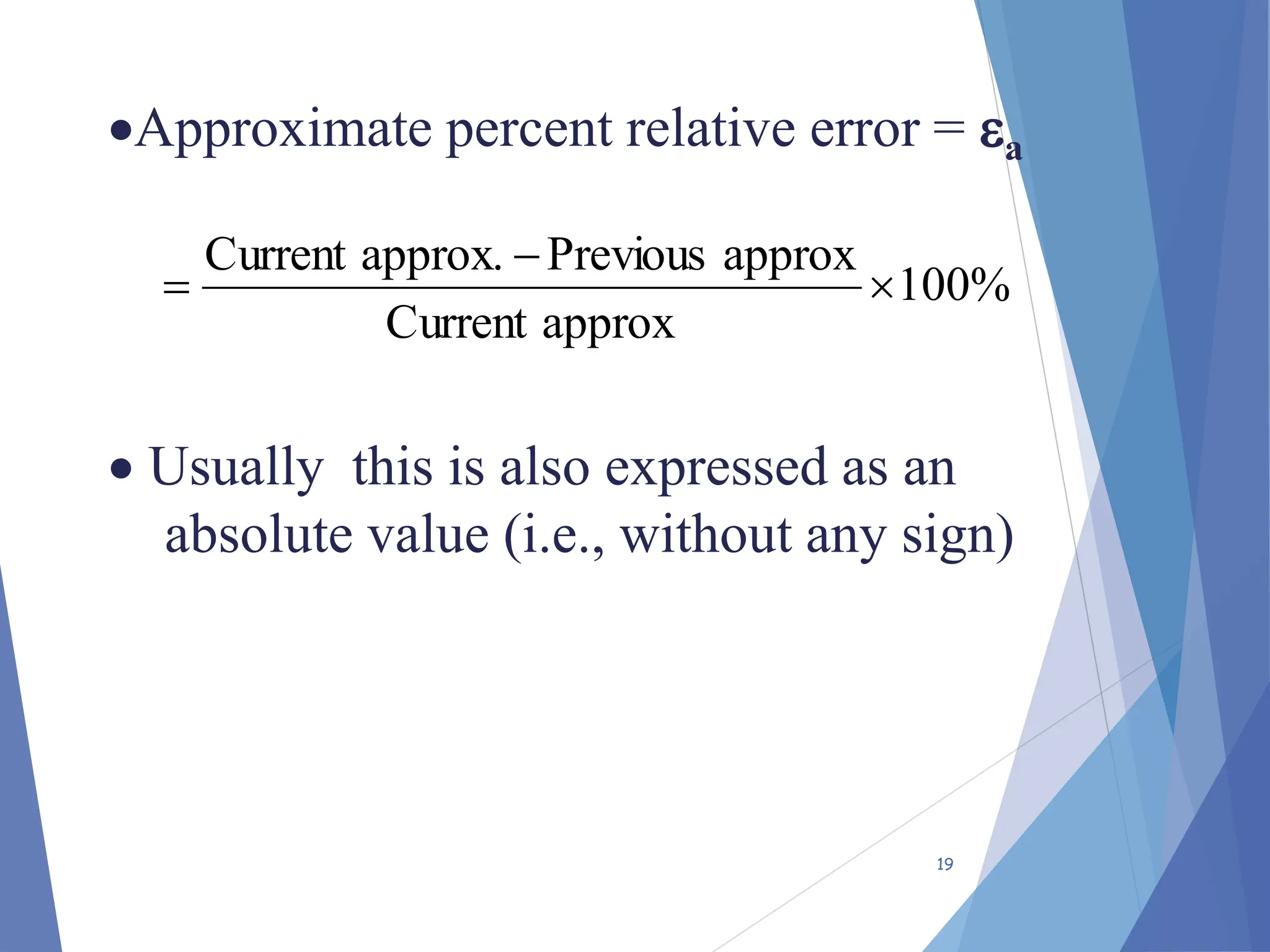
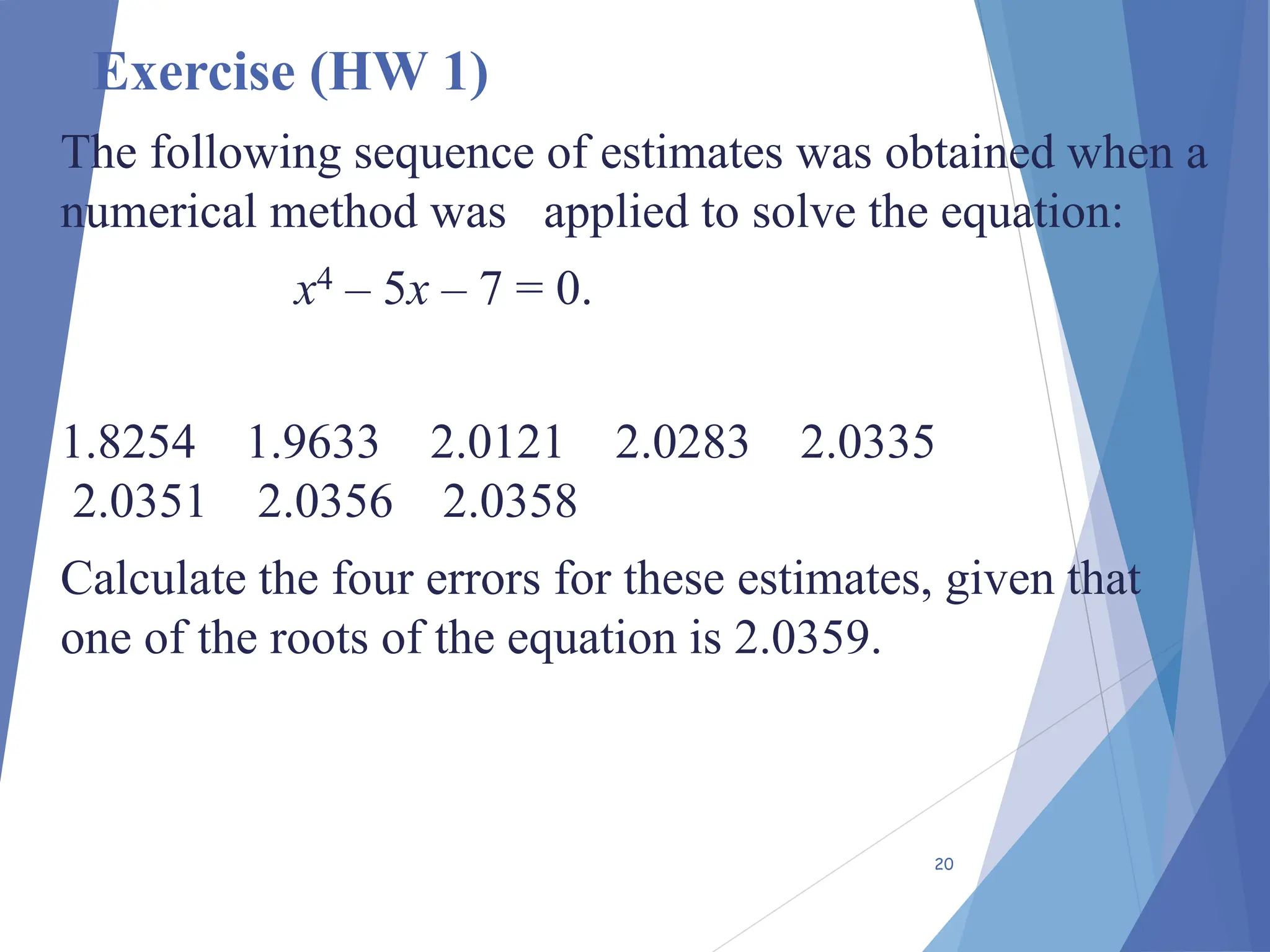
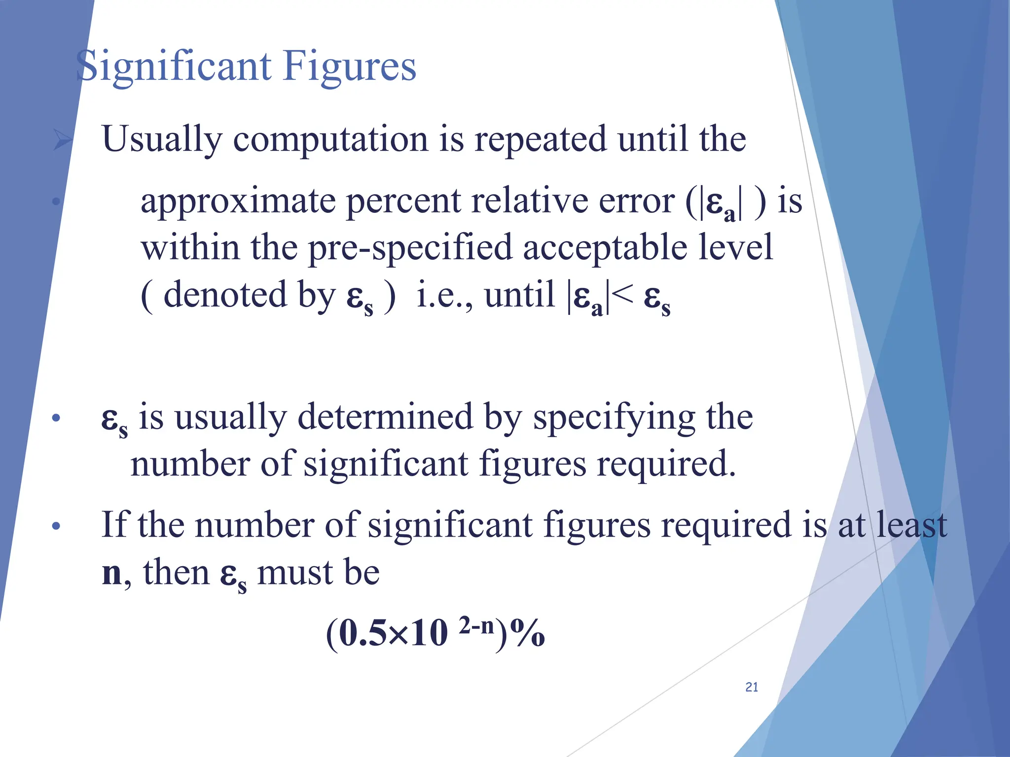
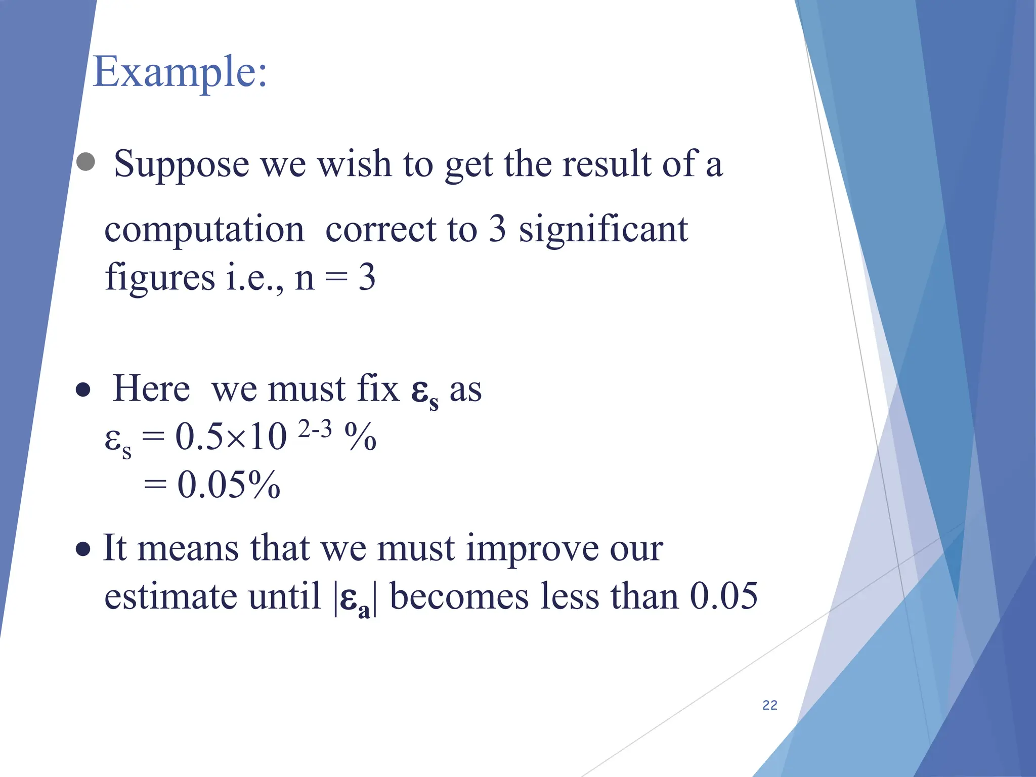
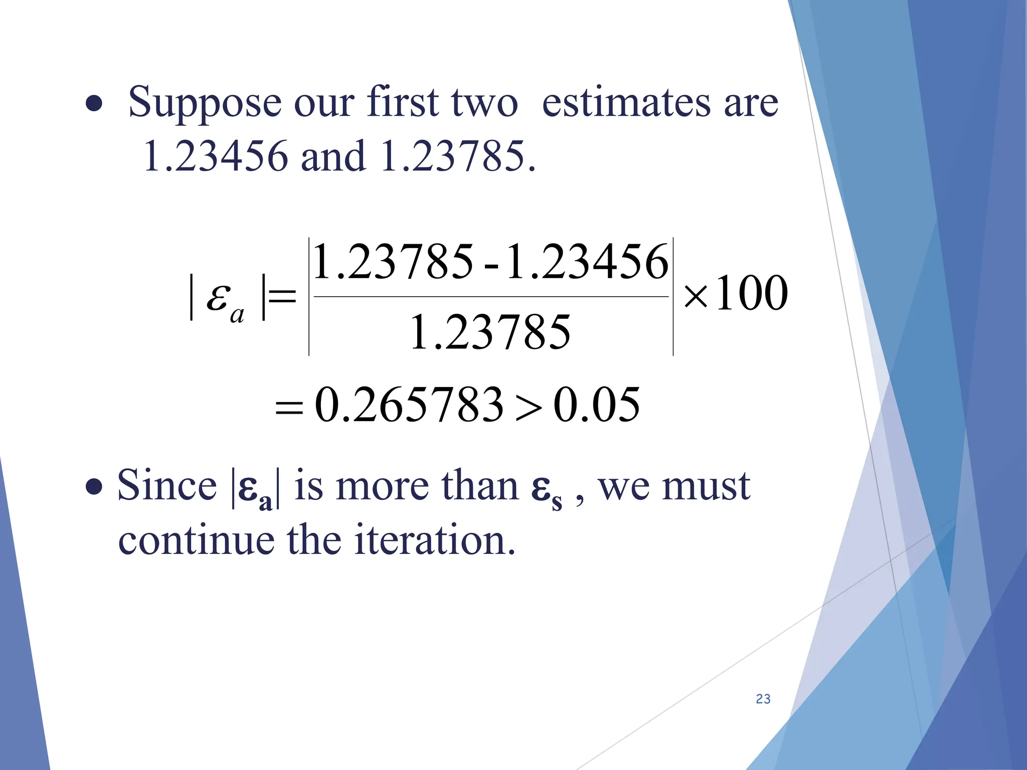
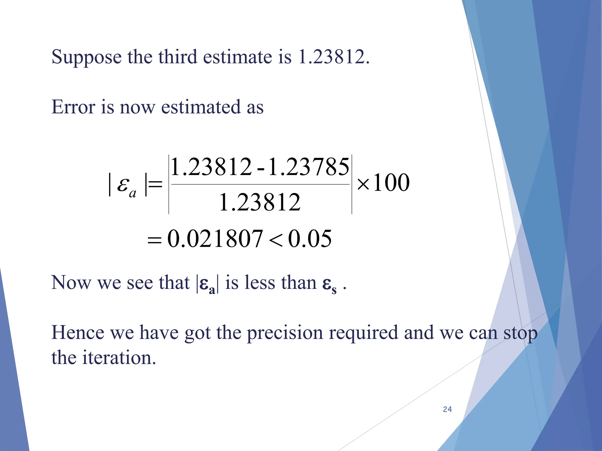
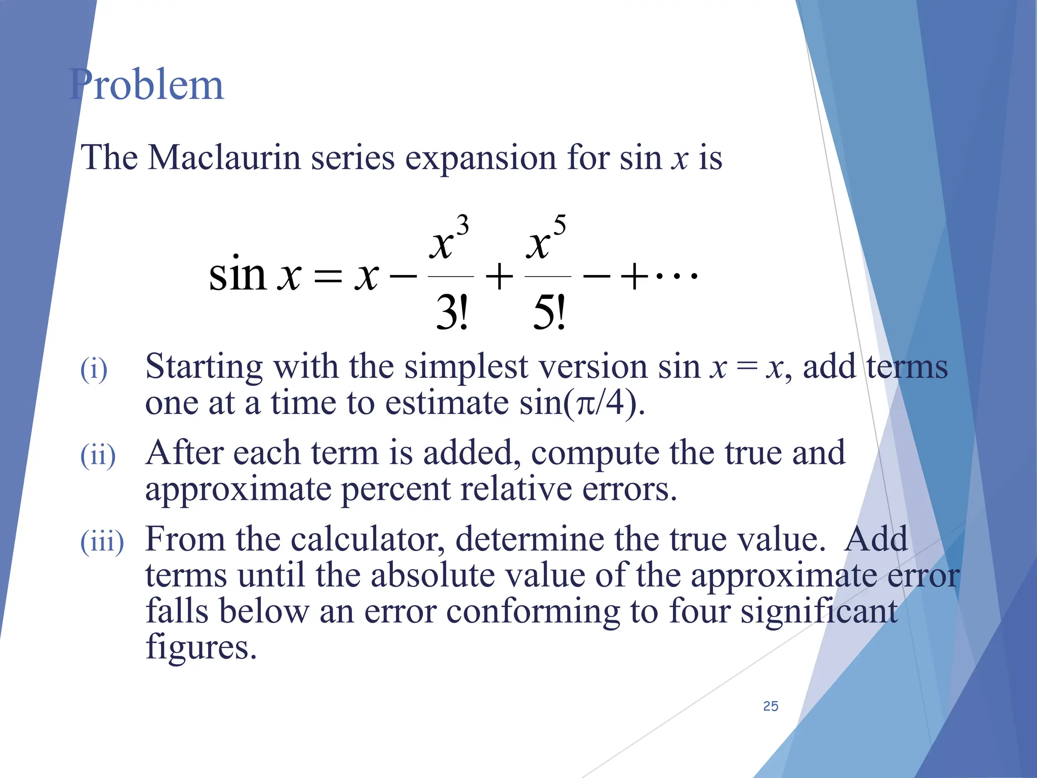
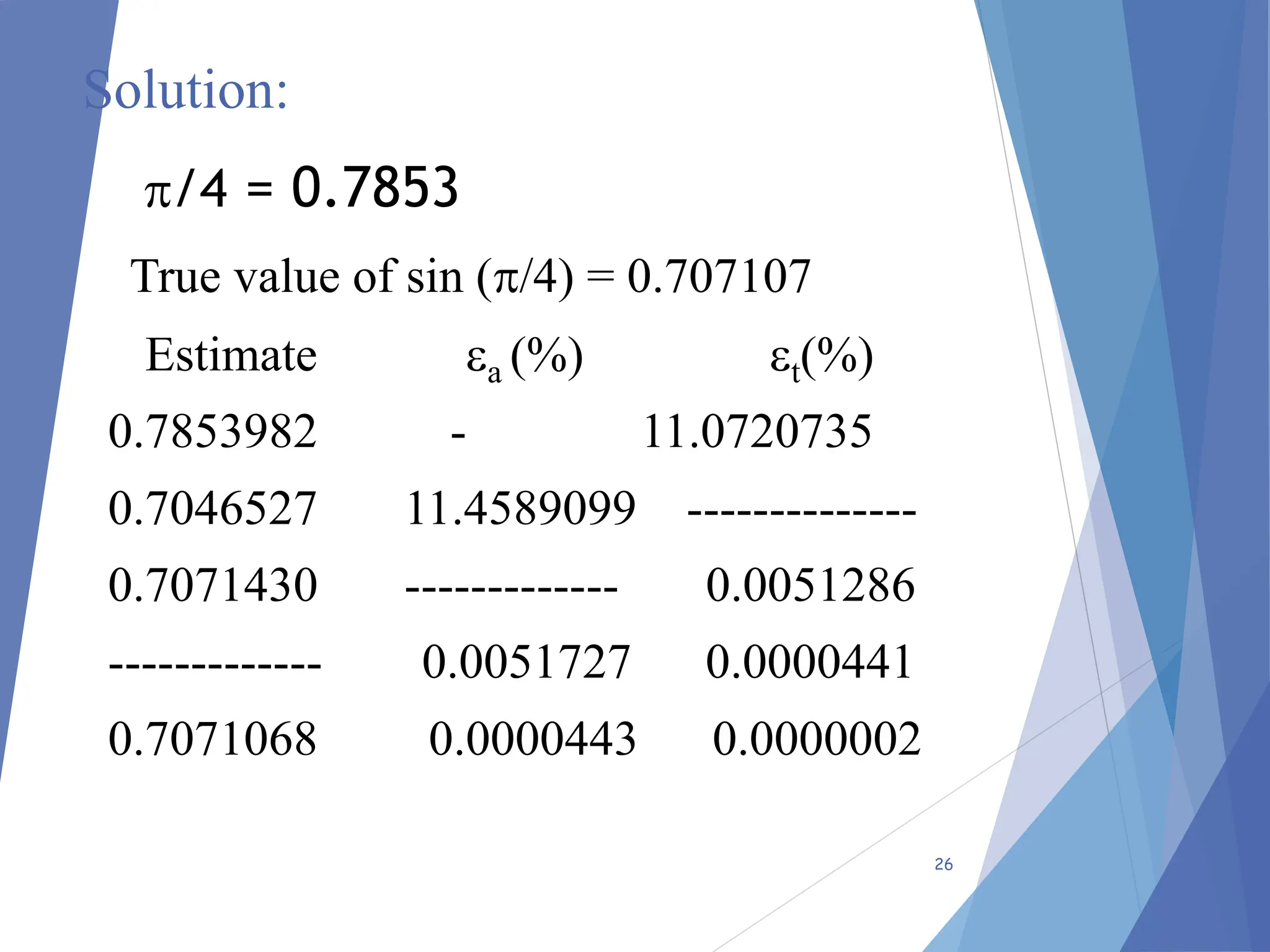
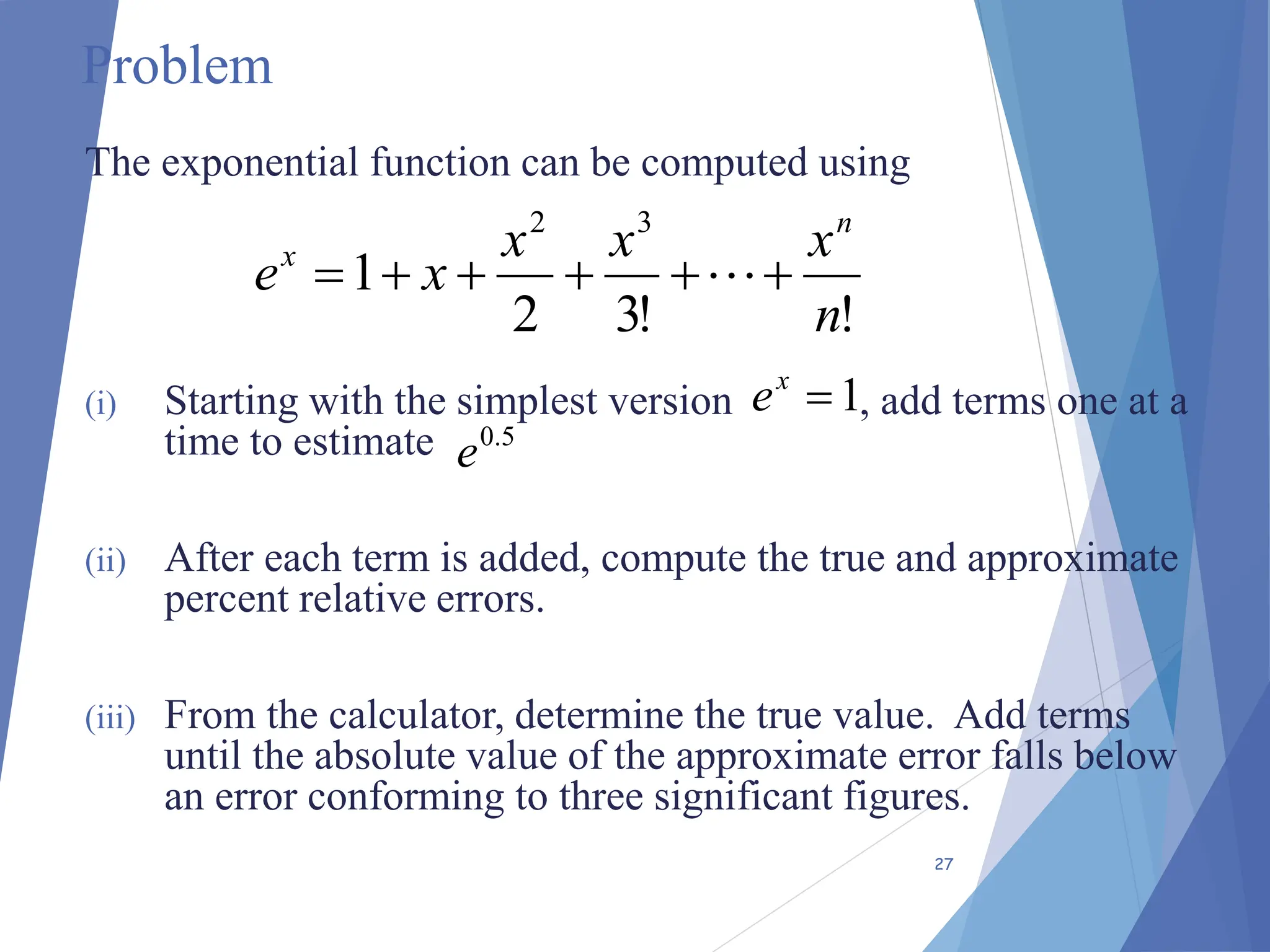
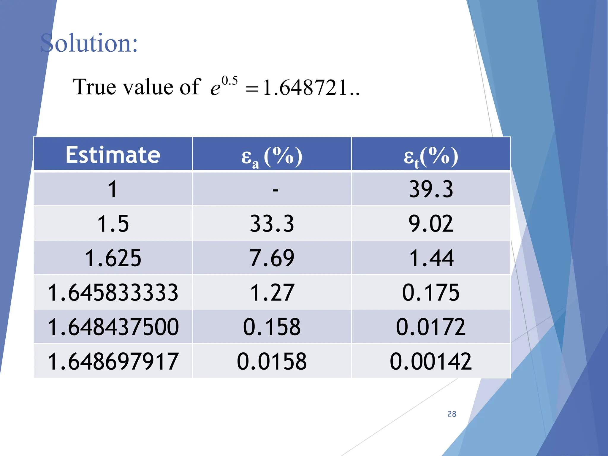
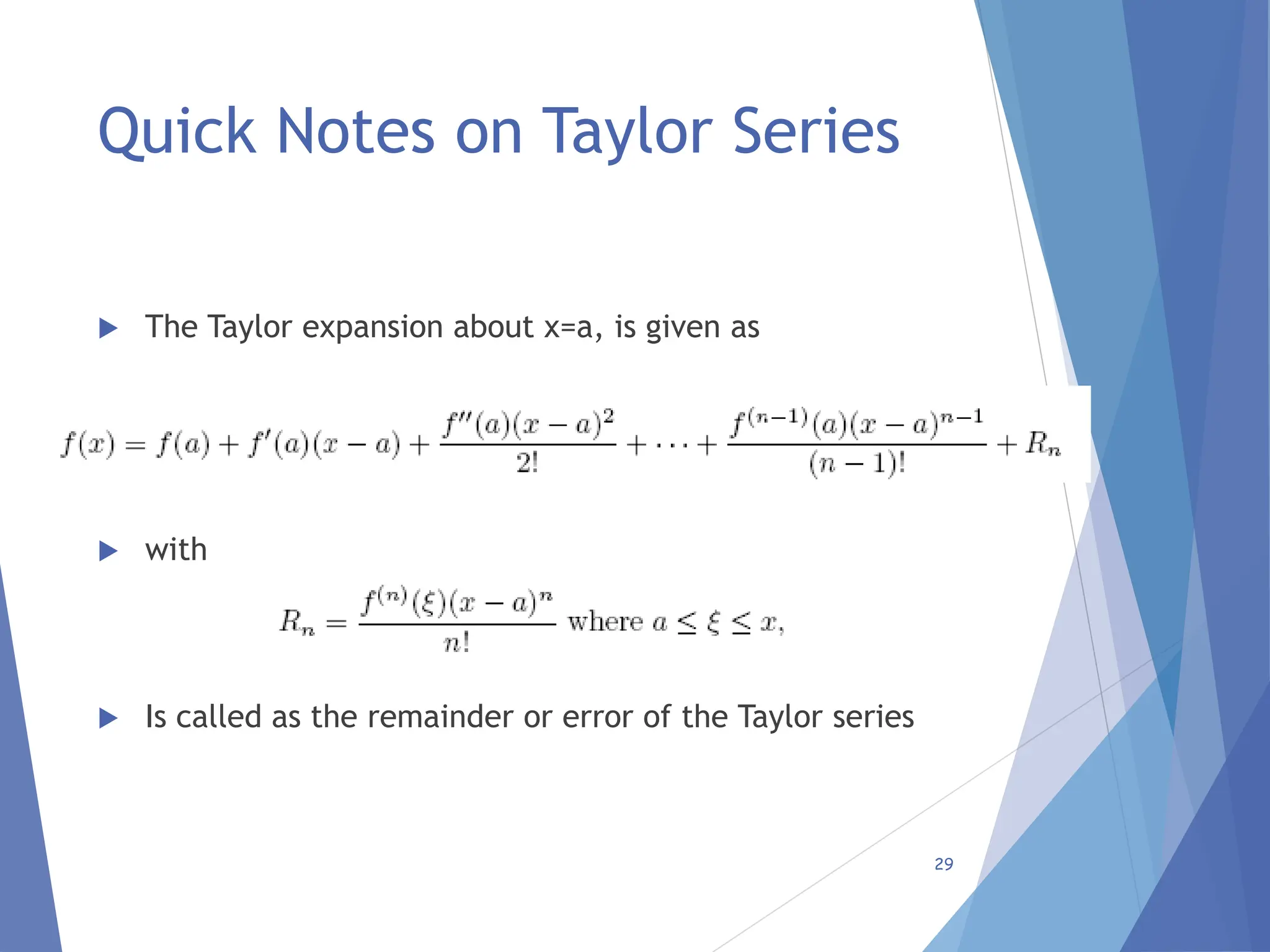
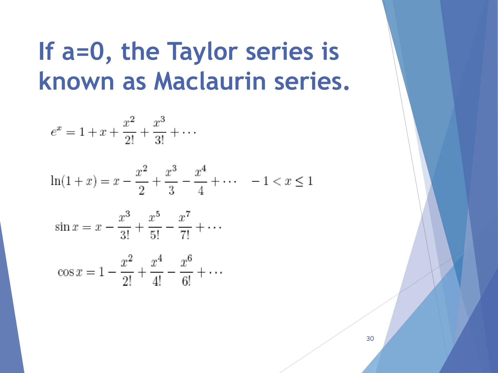
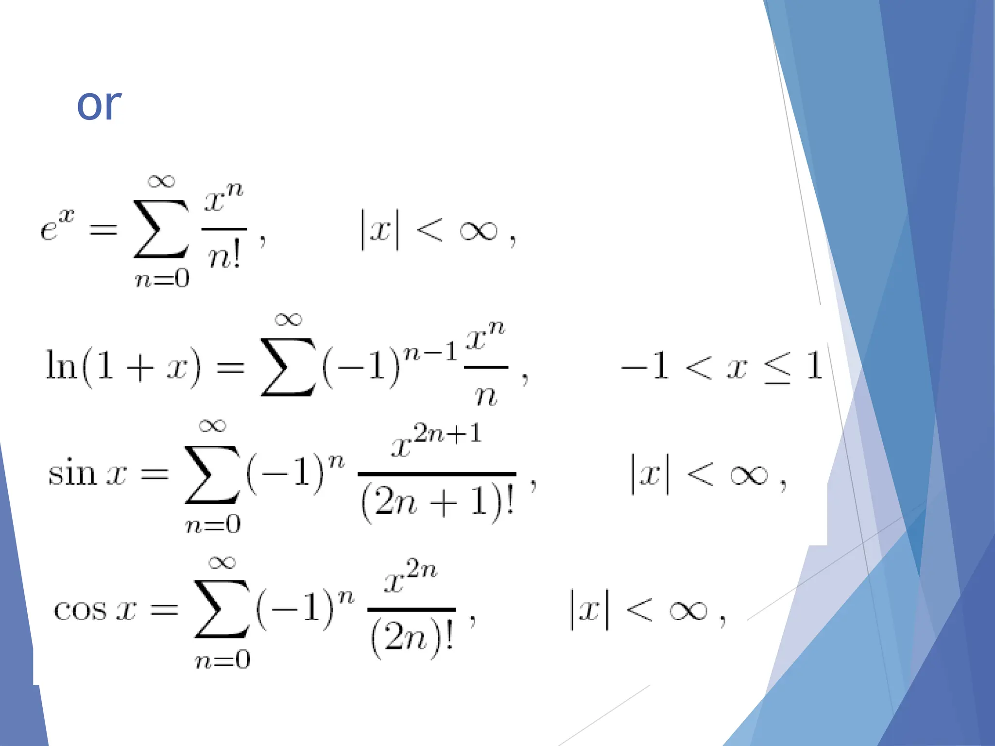
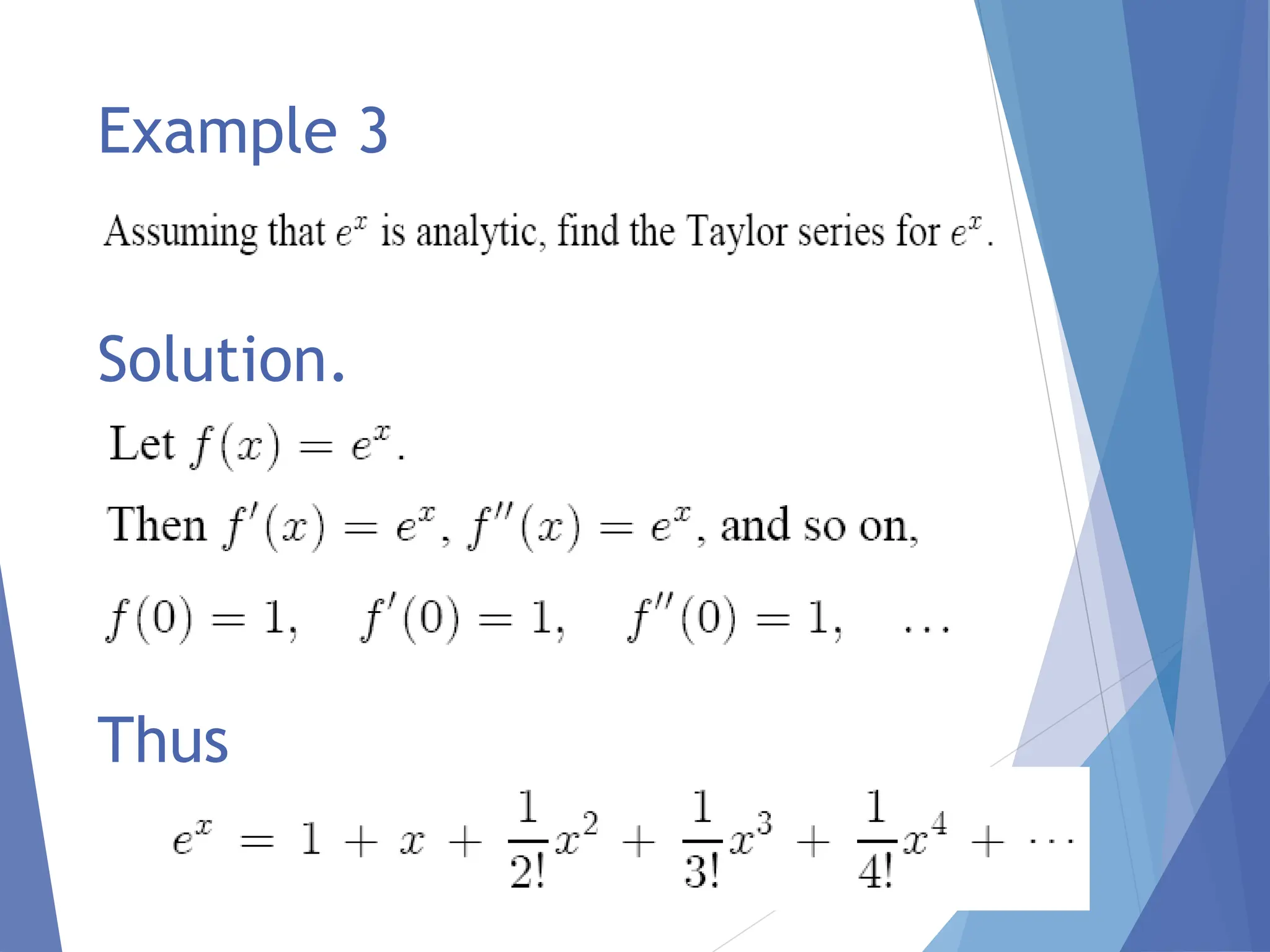
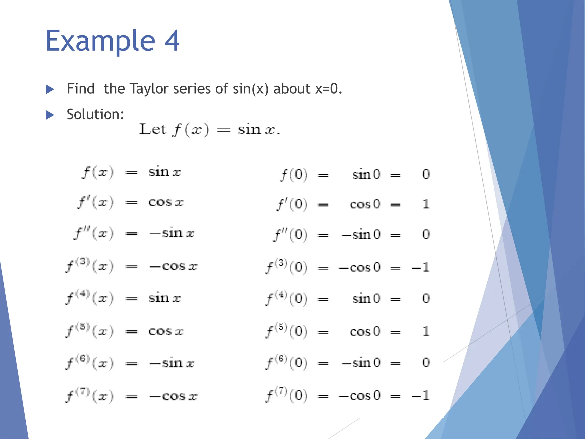
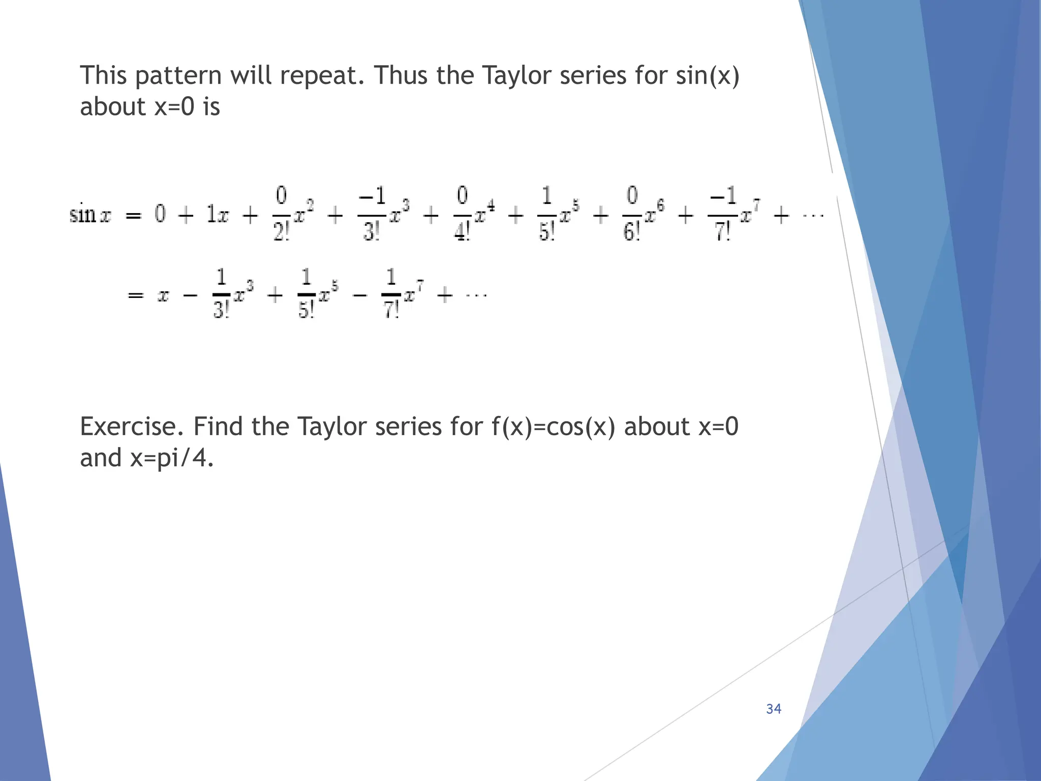
1. NUMERICAL METHODS
FDM 2034:
COMPUTATIONAL METHODS
May 2017
1

2. Introduction to
Numerical Methods
2

3. What is a Numerical Method (NM)?
 A method of solving complex engineering
problems when analytical methods fail to
provide a solution.
 Opposite of NM is Analytical
Method.
3

4. Problem:
Solve the equation: x2 - 3x + 2 = 0
Solutions:
a) Analytical Method:
Using the formula
we get
4
a
ac
b
b
x
2
4
2




1
2
2
8
9
3
or
x 




5. NUMERICAL METHOD
Step 1: Rewrite the equation as x = (x2 + 2)/3
Step 2: Start with some initial solution, say x = 0
Step 3: Using the equation in Step 1, determine x (Here
x = 2/3)
Step 4: Use this value of x to determine the next
approximation.
Step 5: Repeat the process until two successive values
are almost the same.
5

6. Result:
With the equation x = (x2 + 2)/3 and the initial
value x = 0, the successive solutions computed are
as follows:
0, 0.6667, 0.8148, 0.8880, 0.9295, 0.9547,
0.9705, 0.9806, 0.9872, 0.9915,
0.9944, 0.9963, 0.9975, 0.9983, 0.9989,
0.9993, 0.9995,…..
6

7. Important issues in NM
7
APPROXIMATION
errors
accuracy
condition
stability
significant
figures
precision

8. Accuracy vs. Bias
 Accuracy: “…how closely a computed value
agrees with the true value”
 Bias/Inaccuracy : “…a systematic deviation
from the truth”
8
vs.
Accurate Biased/Inaccurate

9. Precision vs. Uncertainty
 Precision : “…how closely individual computed
values agree with each other”
 Uncertainty/Imprecision : “…magnitude of
scatter”
9
vs
.
Precise Uncertain/Imprecise

10. Analogy of a target practice
10
accurate & precise
accurate & imprecise
Inaccurate & precise
Increasing accuracy
Increasing
precision
Inaccurate & imprecise

11. Types of Error
Errors are of two types:
1. Truncation Error
2. Round-off Error
Truncation error is a result of using
approximations to represent exact
mathematical procedures.
Round-off error occurs when only certain
digits and decimal places are used to represent
exact numbers.
11

12. Example 1:
1. We know that
Suppose we use it to evaluate sin 30°.
x = 30°=/6  0.5236
Our first approximation is
sin 30°  0.5236.
12






!
5
!
3
sin
5
3
x
x
x
x

13. Second approximation:
sin 30°  0.5236 - 0.52363/6
= 0.499675
Third approximation:
sin 30°  0.499675+0.52365/120
=0.5000029570
The error involved in the approximations here is
truncation error, since terms in the approximating
series are truncated.
13

14. Example 2:
 Consider the number 3.12746
 If the number is written correct to 3 decimal
places, then it is approximated as 3.127
 If the number is written correct to 4 decimal
places, then it is approximated as 3.1275
 The error involved in this kind of
approximation is called round-off error.
14

15. Measurement of Errors:
 Precision and accuracy are important criteria
for the assessment of approximate solutions.
 There are formulae to measure these
characteristics.
 When the current solution is compared with
the true solution, the error involved is called
true error.
 When the current solution is compared with
the solution obtained in the previous iteration,
the error involved is called approximate error.
15

16. 1. True Error:
• It is used to measure the lack of
accuracy of an estimate.
• True (absolute) error = Et
= True value – Approximation
• True relative error = Et /True value
16

17. True percent relative error = t
 Usually this is expressed as an
absolute value (i.e., without any sign)
17
%
100



value
True
ion
approximat
value
True

18. Approximate Error:
• used to measure the lack of precision of an estimate.
• Approximate (absolute) error
Ea = Current approximation - Previous approximation
• Approximate relative error = Ea/Current app
18

19. Approximate percent relative error = a
 Usually this is also expressed as an
absolute value (i.e., without any sign)
19
%
100
approx
Current
approx
Previous
approx.
Current




20. Exercise (HW 1)
The following sequence of estimates was obtained when a
numerical method was applied to solve the equation:
x4 – 5x – 7 = 0.
1.8254 1.9633 2.0121 2.0283 2.0335
2.0351 2.0356 2.0358
Calculate the four errors for these estimates, given that
one of the roots of the equation is 2.0359.
20

21. Significant Figures
 Usually computation is repeated until the
• approximate percent relative error (|a| ) is
within the pre-specified acceptable level
( denoted by s ) i.e., until |a|< s
• s is usually determined by specifying the
number of significant figures required.
• If the number of significant figures required is at least
n, then s must be
(0.510 2-n)%
21

22. Example:
 Suppose we wish to get the result of a
computation correct to 3 significant
figures i.e., n = 3
 Here we must fix s as
s = 0.510 2-3 %
= 0.05%
 It means that we must improve our
estimate until |a| becomes less than 0.05
22

23.  Suppose our first two estimates are
1.23456 and 1.23785.
 Since |a| is more than s , we must
continue the iteration.
23
0.05
0.265783
100
1.23785
1.23456
-
1.23785
|
|




a


24. Suppose the third estimate is 1.23812.
Error is now estimated as
Now we see that |a| is less than s .
Hence we have got the precision required and we can stop
the iteration.
24
0.05
0.021807
100
1.23812
1.23785
-
1.23812
|
|




a


25. Problem
The Maclaurin series expansion for sin x is
(i) Starting with the simplest version sin x = x, add terms
one at a time to estimate sin(/4).
(ii) After each term is added, compute the true and
approximate percent relative errors.
(iii) From the calculator, determine the true value. Add
terms until the absolute value of the approximate error
falls below an error conforming to four significant
figures.
25






!
5
!
3
sin
5
3
x
x
x
x

26. Solution:
/4 = 0.7853
True value of sin (/4) = 0.707107
Estimate a (%) t(%)
0.7853982 - 11.0720735
0.7046527 11.4589099 --------------
0.7071430 ------------- 0.0051286
------------- 0.0051727 0.0000441
0.7071068 0.0000443 0.0000002
26

27. Problem
The exponential function can be computed using
(i) Starting with the simplest version , add terms one at a
time to estimate
(ii) After each term is added, compute the true and approximate
percent relative errors.
(iii) From the calculator, determine the true value. Add terms
until the absolute value of the approximate error falls below
an error conforming to three significant figures.
27
!
!
3
2
1
3
2
n
x
x
x
x
e
n
x





 
1

x
e
5
.
0
e

28. Solution:
True value of
28
..
648721
.
1
5
.
0

e
Estimate a (%) t(%)
1 - 39.3
1.5 33.3 9.02
1.625 7.69 1.44
1.645833333 1.27 0.175
1.648437500 0.158 0.0172
1.648697917 0.0158 0.00142

29. Quick Notes on Taylor Series
 The Taylor expansion about x=a, is given as
 with
 Is called as the remainder or error of the Taylor series
29

30. If a=0, the Taylor series is
known as Maclaurin series.
30

31. or
31

32. Example 3
Solution.
Thus
32

33. Example 4
 Find the Taylor series of sin(x) about x=0.
 Solution:
33

34. 34
This pattern will repeat. Thus the Taylor series for sin(x)
about x=0 is
Exercise. Find the Taylor series for f(x)=cos(x) about x=0
and x=pi/4.