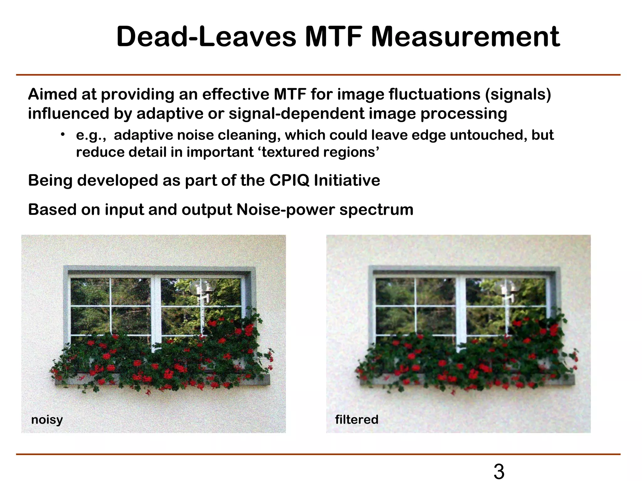
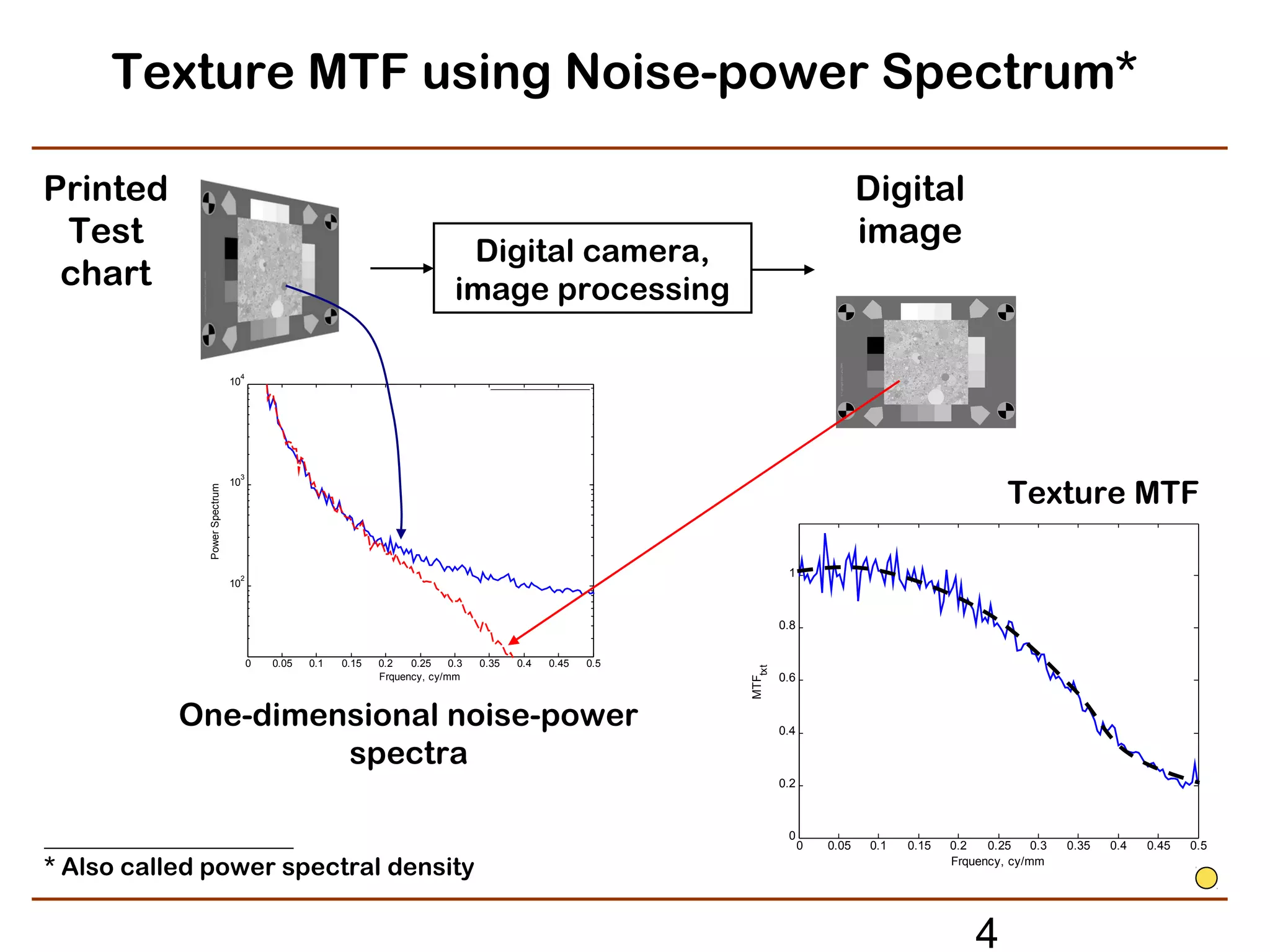
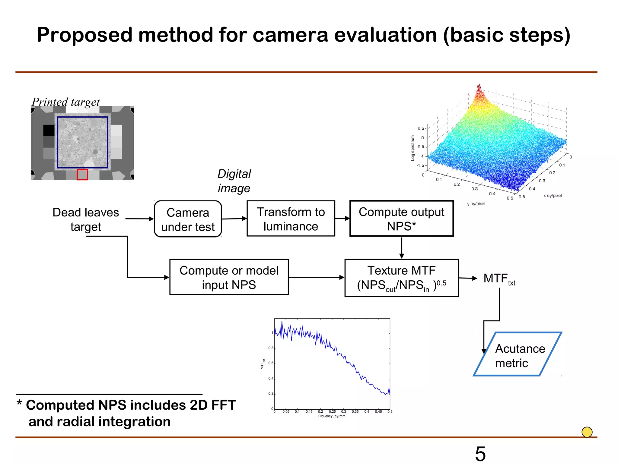
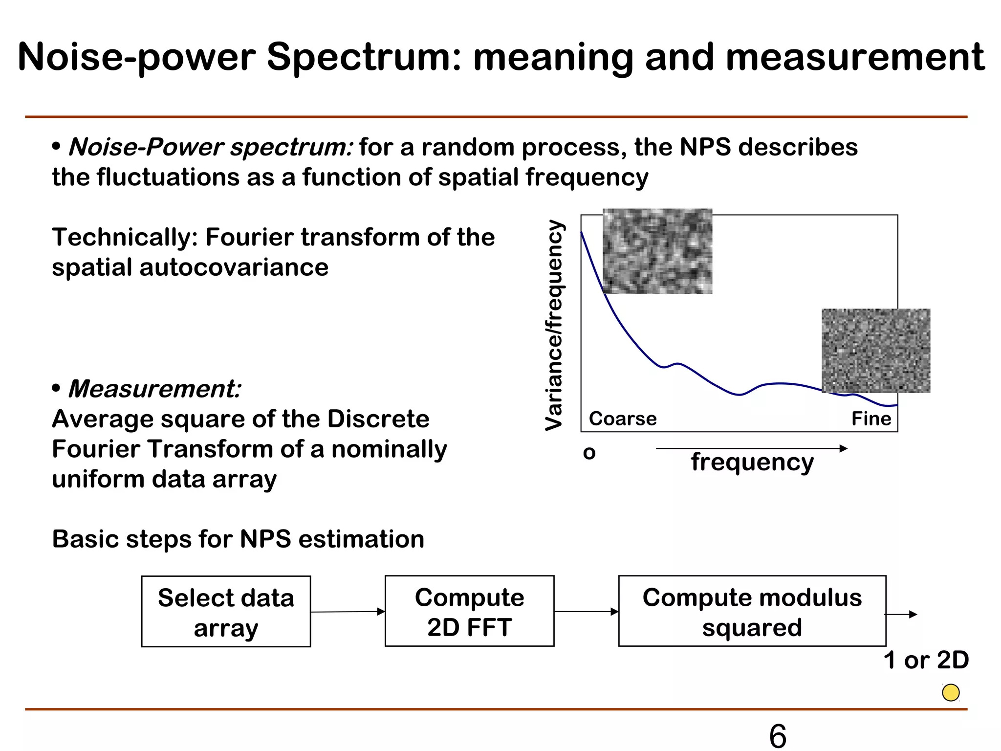
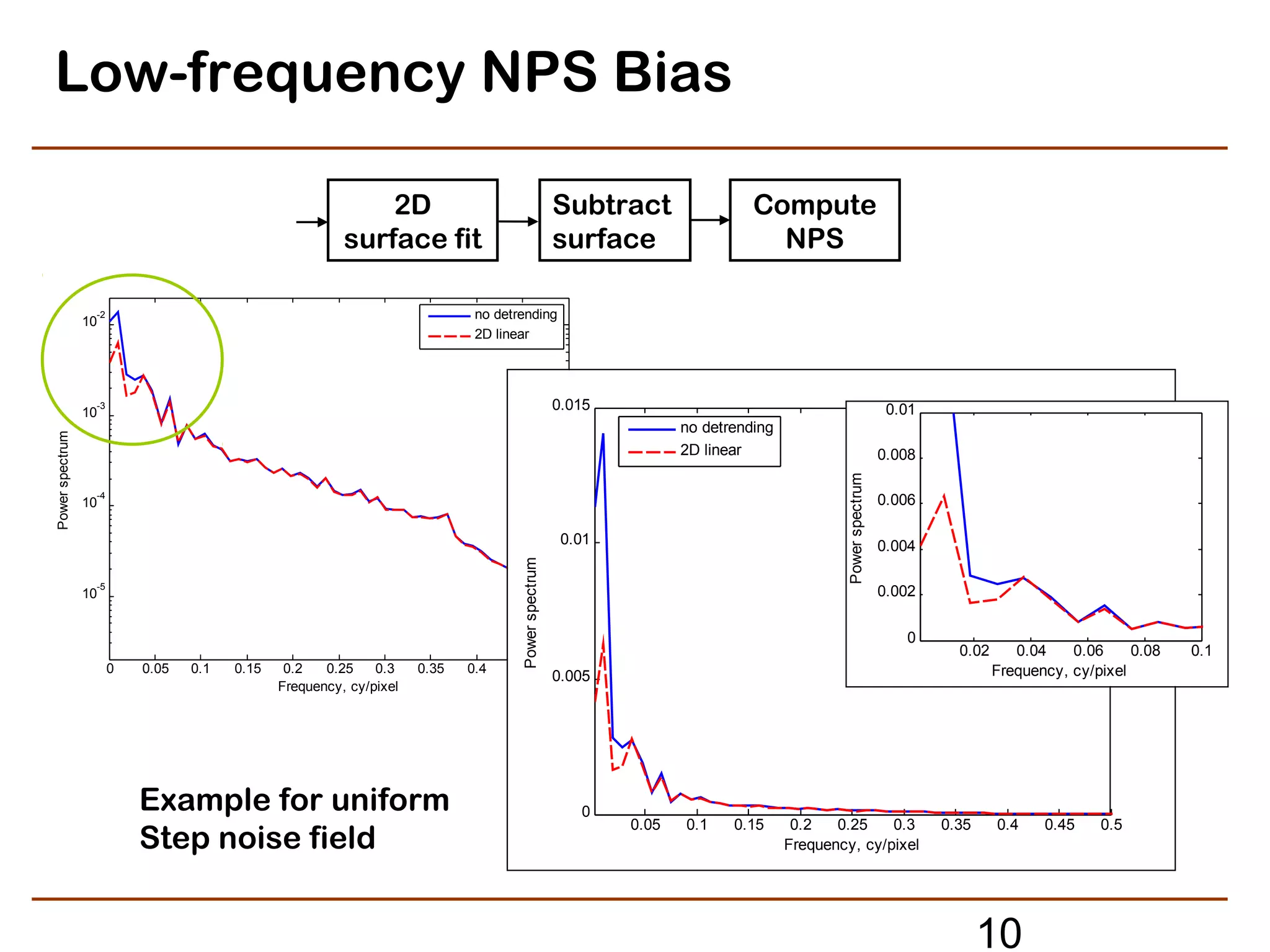
The document discusses refined methods for measuring digital image texture loss using targets with random objects. Specifically, it proposes measuring texture modulation transfer function (MTF) based on analyzing the noise power spectrum of input and output images. This approach aims to provide an effective MTF measure for image areas influenced by adaptive or signal-dependent processing, such as noise cleaning. Key steps involve computing the noise power spectrum of a noisy input target image, applying the imaging system or processing under test, and computing the output noise power spectrum to determine the texture MTF. The method seeks to provide a practical texture loss measurement but must address random and bias errors introduced during estimation of noise power spectra.

1. Refined Measurement of Digital
Image Texture Loss
50
100
150
200
250
300
350 Peter D. Burns
400
450
500
Burns Digital Imaging
100 200 300 400 500
Reference:
P.D. Burns, Refined Measurement of Digital Image Texture Loss, Proc. SPIE Vol. 8653,
Image Quality and System Performance X, 86530H, 2013
IS&T and SPIE Electronic Imaging Symposium, Jan. 2013

2. Introduction
Texture-loss MTF using targets with random objects
• Dead-leaves target analysis based on noise-power spectrum
Previously applied to image detail loss during; image capture,
noise-cleaning, image compression
Method is based on noise-power spectrum (NPS) estimation
Practical measurement introduces random and bias estimation-
error, e.g. non-stationary statistics
Common source can be corrected for, reducing measurement
error
NPS, Texture MTF and computed acutance measures are
improved
Acknowledgements: Uwe Artmann, Donald Baxter, Frédéric Cao, Herve
Hornung, Norman Koren, Don Williams and Dietmar Wueller
2

3. Dead-Leaves MTF Measurement
Aimed at providing an effective MTF for image fluctuations (signals)
influenced by adaptive or signal-dependent image processing
• e.g., adaptive noise cleaning, which could leave edge untouched, but
reduce detail in important ‘textured regions’
Being developed as part of the CPIQ Initiative
Based on input and output Noise-power spectrum
noisy filtered
3

4. Texture MTF using Noise-power Spectrum*
Printed Digital
Test image
Digital camera,
chart image processing
4
10
Input target
JPEG 2000
Texture MTF
3
10
Power Spectrum
2
1
10
0.8
0 0.05 0.1 0.15 0.2 0.25 0.3 0.35 0.4 0.45 0.5
MTFtxt
Frquency, cy/mm 0.6
One-dimensional noise-power 0.4
spectra
0.2
____________________ 0
0 0.05 0.1 0.15 0.2 0.25 0.3 0.35 0.4 0.45 0.5
* Also called power spectral density Frquency, cy/mm
4

5. Proposed method for camera evaluation (basic steps)
Printed target
Digital
image
Dead leaves Camera Transform to Compute output
target under test luminance NPS*
Compute or model Texture MTF
MTFtxt
input NPS (NPSout/NPSin )0.5
1
0.8
Acutance
metric
MTFtxt
0.6
0.4
___________________________ 0.2
* Computed NPS includes 2D FFT 0
0 0.05 0.1 0.15 0.2 0.25 0.3 0.35 0.4 0.45 0.5
and radial integration
Frquency, cy/mm
5

6. Noise-power Spectrum: meaning and measurement
• Noise-Power spectrum: for a random process, the NPS describes
the fluctuations as a function of spatial frequency
Variance/frequency
Technically: Fourier transform of the
spatial autocovariance
• Measurement:
Average square of the Discrete Coarse Fine
Fourier Transform of a nominally o frequency
uniform data array
Basic steps for NPS estimation
Select data Compute Compute modulus
array 2D FFT squared
1 or 2D
6

7. Noise-power spectrum measurement
• Noise-power spectrum is a second-order parameter of
a stochastic process
• NPS measurement is a statistical estimate that relies
on stable (stationary) statistics
- constant mean and variance
• Image nonuniformity (falloff) causes a bias error in
NPS estimates
• Lens shading, lighting variation etc.
NPS error MTF error
7

8. Variance estimation bias
1.5 1.5 1.5
1 1 1
0.5 0.5 0.5
0 0 0
-0.5 -0.5 -0.5
-1 -1 -1
-1.5 -1.5 -1.5
0 5 10 15 20 25 30 35 40 45 50 0 5 10 15 20 25 30 35 40 45 50 0 5 10 15 20 25 30 35 40 45 50
Variance estimate N N
1 1
s2 = ∑ ∆xi2 ∆xi = xi −
N
∑ xi s 2 ≅ σ 2 , N large
N i =1 i =1
Random signal plus trend xi' = xi + f i
Biased variance estimate Es [ ] 2 2
=σx +
1
N
N
∑ fi2
i =1
bias
Standard deviation 0.23 0.43
8

9. Bias error and improving estimation
• Estimation error can be measured
• If sources are known, estimates can be improved
Examples; instrument calibration, seasonal adjustments
• Nonuniform mean value biases noise estimates
Variance, standard deviation, noise-power spectrum
• Objective: design improved NPS estimate that is
simple and benign (does not over-compensate)
• Instead of subtracting the sample mean value,
subtract a 2D plane (linear fit) function
2D Subtract Compute
surface fit surface NPS
9

10. Low-frequency NPS Bias
2D Subtract Compute
surface fit surface NPS
-2 no detrending
10
2D linear
-3
10
0.015 0.01
no detrending
Power spectrum
2D linear 0.008
Power spectrum
-4
10 0.006
0.01 0.004
Power spectrum
-5
10 0.002
0
0.02 0.04 0.06 0.08 0.1
0 0.05 0.1 0.15 0.2 0.25 0.3 0.35 0.4 0.45 0.5 Frequency, cy/pixel
0.005
Frequency, cy/pixel
Example for uniform 0
Step noise field
0.05 0.1 0.15 0.2 0.25 0.3 0.35 0.4 0.45 0.5
Frequency, cy/pixel
10

11. Signal
input 2D fit
50 50
100 100
150 150
200 200
250 250
300 300
350 350
400 400
450 450
500 500
100 200 300 400 500 100 200 300 400 500
output
50
100
150
200
250
300
350
400
450
500
100 200 300 400 500
After subtraction of 2d fit, plane, computed RMS noise reduced 7%
11

12. Noise-corrected Texture NPS
Noise-corrected dead leaves NPS, with and without 2D linear
trend removal
% difference due to detrending
15
0
10 Noise
Texture signal
Corrected 10
-1
10
5
NPS % difference
Power Spectrum
-2
10
0
-3
10
-5
-4
10
-10
-15
0 0.05 0.1 0.15 0.2 0.25 0.3 0.35 0.4 0.45 0.5 0 0.02 0.04 0.06 0.08 0.1 0.12 0.14 0.16 0.18 0.2
Frequency, cy/pixel Frequency, cy/pixel
12

13. Texture-MTF Results from Camera Testing
NPS error MTF error
Mean relative error reduction (N=5 replicates)
• All frequencies [0, 0.5 cy/pixel] 20%.
• Low frequencies [0, 2.5 cy/pixel] 26%.
1.2 1.2
1 1
0.8 0.8
txt
MTFtxt
MTF
0.6 0.6
0.4 0.4
0.2 0.2
0 0
0 0.05 0.1 0.15 0.2 0.25 0.3 0.35 0.4 0.45 0.5 0 0.05 0.1 0.15 0.2 0.25 0.3 0.35 0.4 0.45 0.5
Frquency, cy/mm Frquency, cy/mm
no trend removal 2D-linear fit and subtraction
Final scaling was done at 0.02 cy/pixel
13

14. Summary
1. Noise-power spectrum (NPS) is a (second-order) statistical
measure
2. Measuring a statistic is estimation
3. Good estimation relies on stable (stationary) population
statistics
4. Image nonuniformity leads to NPS bias (positive at low
frequencies) and variation
5. Simple 2D detrending (subtract a plane rather than a sample
mean value) reduces bias and variation in the NPS estimate.
6. This is a pre-processing step that can be done before NPS
estimation
7. This leads to reduced estimation error in the texture MTF,
which is computed from (is a function of) two NPS estimates
NPS error Texture MTF error
14

15. Conclusions
Proposed texture MTF analysis relies on noise-power
spectrum (NPS) estimation
We investigated error introduced into NPS by non-
stationary (mean) signal
Benign and simple correction two-dimensional by de-
trending of image data array
Reduction in low-frequency bias and variation (20%)
pdburns@ieee.org
15

16. Mobile camera example (not presented at EI)
• Test image files from N. Koren
• NPS estimation with and without detrending
• Very little difference
Camera A 50 50
100
Camera B 100
150 150
200 200
250 250
300 300
350 350
400 400
450 450
500 500
100 200 300 400 500 100 200 300 400 500
15 6
no detrending no detrending
2D linear 2D linear
5
10 4
Power spectrum
Power spectrum
3
5 2
1
0 0
0.01 0.02 0.03 0.04 0.05 0.06 0.07 0.08 0.09 0.1 0.01 0.02 0.03 0.04 0.05 0.06 0.07 0.08 0.09 0.1
Frequency, cy/pixel Frequency, cy/pixel
16

17. Camera comparison by texture MTF
Effective texture MTF, camera A is the
reference (input). Acutance = 0.73
2
10 1.8
1 1.6
10
1.4
NPS
0
10
1.2
-1
10
1
MTFtxt
-2
10
0.8
-3
10
0.6
-4
10
0.4
-5
10 0.2
-6
10 0
0 0.1 0.2 0.3 0.4 0.5 0.6 0.7 0 0.1 0.2 0.3 0.4 0.5 0.6
Frquency, cy/mm
Frequency, cy/mm
17