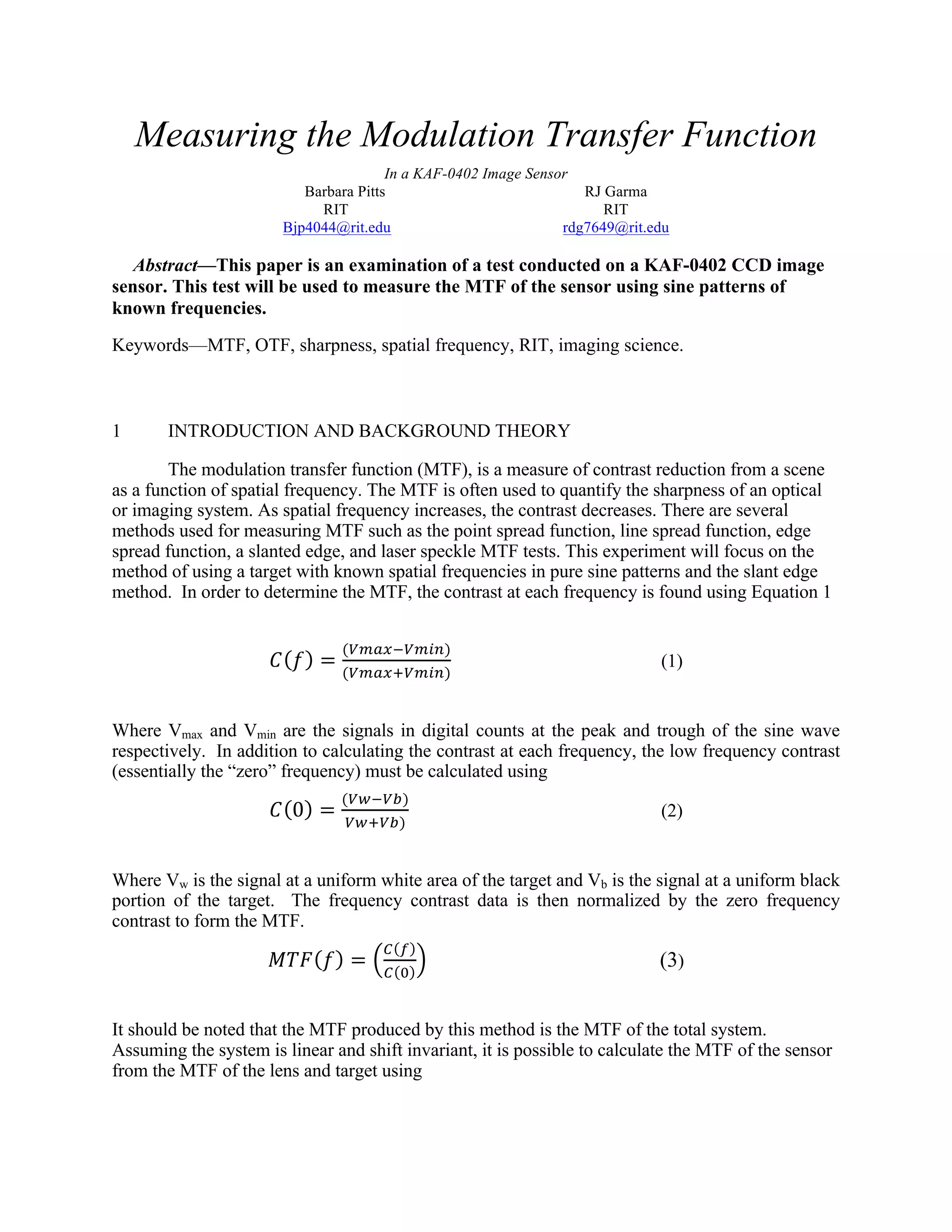
1. Measuring the Modulation Transfer Function
In a KAF-0402 Image Sensor
Barbara Pitts RJ Garma
RIT RIT
Bjp4044@rit.edu rdg7649@rit.edu
Abstract—This paper is an examination of a test conducted on a KAF-0402 CCD image
sensor. This test will be used to measure the MTF of the sensor using sine patterns of
known frequencies.
Keywords—MTF, OTF, sharpness, spatial frequency, RIT, imaging science.
1 INTRODUCTION AND BACKGROUND THEORY
The modulation transfer function (MTF), is a measure of contrast reduction from a scene
as a function of spatial frequency. The MTF is often used to quantify the sharpness of an optical
or imaging system. As spatial frequency increases, the contrast decreases. There are several
methods used for measuring MTF such as the point spread function, line spread function, edge
spread function, a slanted edge, and laser speckle MTF tests. This experiment will focus on the
method of using a target with known spatial frequencies in pure sine patterns and the slant edge
method. In order to determine the MTF, the contrast at each frequency is found using Equation 1
𝐶 𝑓 =
(!"#$!!"#$)
(!"#$!!"#$)
(1)
Where Vmax and Vmin are the signals in digital counts at the peak and trough of the sine wave
respectively. In addition to calculating the contrast at each frequency, the low frequency contrast
(essentially the “zero” frequency) must be calculated using
𝐶 0 =
(!"!!")
!"!!")
(2)
Where Vw is the signal at a uniform white area of the target and Vb is the signal at a uniform black
portion of the target. The frequency contrast data is then normalized by the zero frequency
contrast to form the MTF.
𝑀𝑇𝐹 𝑓 =
! !
! !
(3)
It should be noted that the MTF produced by this method is the MTF of the total system.
Assuming the system is linear and shift invariant, it is possible to calculate the MTF of the sensor
from the MTF of the lens and target using

2. 𝑀𝑇𝐹! =
!!
!!∗!"#!
(4)
MTFs is the sensor MTF, Mi is the modulation of the image, Mt is the modulation of the target,
and MTFl is the lens MTF.
In addition to using sine wave targets, the MTF of the system may be derived from a slant edge.
A slant edge target offers improvements in performance over a standard vertical or horizontal
edge by project pixels on to the edge, in effect achieving super-resolution over the edge spread
function (ESF). This process is illustrated in the figure below.
(a) (b)
(c) (d)
Figure 1: a) Sampling from first row of pixels b) sampling from second row of pixels c) sampling from third
row of pixels d) Combined sampling of ESF.
The line spread function (LSF) is generated by taking the derivative of the ESF, and lastly the
MTF is found by taking the Fourier Transform of the LSF (Fig. 2).

3. (a) (b)
(c)
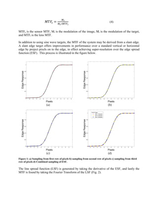
Figure 2: a) Super-sampled edge spread function b) Line spread function c) Modulation transfer function.
Assuming square pixels and a fill factor of one, the pixel pitch (sampling distance between
pixels) is estimated to be the pixel width (physical dimension of the pixel). From this
assumption, the nyquist frequency is calculated by
𝑓!"#$%&'[
!"!!"#
!!
] =
!
!!
(5)
where p is the pixel width in millimeters.
2 Experimental Procedure
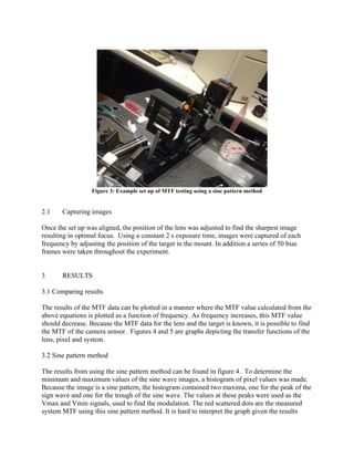
2.1 Experimental Set up
For this experiment a 90mm Fuji enlarger lens is used. This lens does not mount to the CCD
camera itself, so alignment into the optical path was necessary. The target being used is a glass,
backlit sine pattern frequency target with varying frequencies. The camera, lens, and target were
mounted onto an optical rail which allowed for adjustments along the z-axis. Using Equation 1
and a 1:1 magnification requirement, the distance to the object (Do) and image (Di) were found to
be 180mm, or approximately 7in. An image of the testing set up is shown in Figure 3. A green
filter was placed in between the lens and the sine pattern resulting in narrow band light centered
about 540nm. Furthermore, the camera was cooled to minimize the contribution of dark current.
!
!
=
!
!!
+
!
!!
(6)

4. Figure 3: Example set up of MTF testing using a sine pattern method
2.1 Capturing images
Once the set up was aligned, the position of the lens was adjusted to find the sharpest image
resulting in optimal focus. Using a constant 2 s exposure time, images were captured of each
frequency by adjusting the position of the target in the mount. In addition a series of 50 bias
frames were taken throughout the experiment.
3 RESULTS
3.1 Comparing results
The results of the MTF data can be plotted in a manner where the MTF value calculated from the
above equations is plotted as a function of frequency. As frequency increases, this MTF value
should decrease. Because the MTF data for the lens and the target is known, it is possible to find
the MTF of the camera sensor. Figures 4 and 5 are graphs depicting the transfer functions of the
lens, pixel and system.
3.2 Sine pattern method
The results from using the sine pattern method can be found in figure 4. To determine the
minimum and maximum values of the sine wave images, a histogram of pixel values was made.
Because the image is a sine pattern, the histogram contained two maxima, one for the peak of the
sign wave and one for the trough of the sine wave. The values at these peaks were used as the
Vmax and Vmin signals, used to find the modulation. The red scattered dots are the measured
system MTF using this sine pattern method. It is hard to interpret the graph given the results

5. calculated using the measured system MTF and the measured pixel MTF, which could be due to
a number of reasons that will be discussed later. The blue data points are the modulation of the
signal as a function of frequency, which behaves in the expected way. The measured system
MTF (red data points) is found by dividing the normalized image modulation by the target MTF.
These points are found to deviate from the expected trend and also do not match the theoretical
system MTF. The measured pixel MTF (green dots) is calculated by dividing the measured
system MTF by the lens MTF. These points were also found to deviate greatly from the
theoretical pixel MTF, modeled as a SINC function. Assuming a fill factor of one (pixel pitch =
pixel size), the Nyquist was calculated to be 55 cycles/mm.
Figure 4: MTF’s using the sine pattern method
3.3 Slant edge method
Data gathered using the slant edge method appears to be more accurate. Figure 5 is a depiction
of slanted edge MTF data. The SINC model for the pixel MTF is plotted in the thin blue line,
along with the lens MTF as the red line. The theoretical system MTF (lens MTF times pixel
MTF) is plotted here again in the black line. The Slant edge MTF data shown in the green
scattered dots follows the trend much more precisely than the sine method system MTF. The
measured system MTF still appears to be much lower than the theoretical, indicating that
additional factors are affecting the performance of the camera. It was postulated that defocus
may be the primary factor affecting the measured data. A defocus aberration was applied that
minimized the error between the theoretical MTF and the measured MTF, seen as the thick blue
line. The pixel MTF (red dots) was then found by dividing out the defocus aberration and lens
MTF. The resulting measured pixel MTF still deviates greatly from the theoretical pixel MTF
indicating that other factors are still unaccounted for. Furthermore, the defocus aberration

6. contains zeros causing erroneous points in the measure data after dividing out the defocus
aberration.
Figure 5: MTF’s found using the slant edge method
4 CONCLUSIONS
It is concluded that measuring the MTF of a system can be extremely difficult with limited
resources. The hardest part of conducting an experiment of this caliber is optical alignment. It is
imperative that the sensor, lens, and target are perfectly aligned in order to achieve accurate data.
The inaccuracy of the data collected here is most likely due to the fact that the target had to be
moved each time a new frequency needed to be imaged, which most likely resulted in
misalignment in the optical path. Because live view is not possible with a set up like this, focus
was also very hard to achieve. Focus could only be achieved by moving a piece of the system, in
this case the lens, until the image being captured appeared to be in focus. This however could
have changed due to any part of the system being moved by the slightest amount. While it is
believed that accurate data regarding the system MTF as a whole, it is much harder to factor out
sensor MTF data due to inconsistencies in the target images. This could be contributed to the fact
that the target may have not been perfectly perpendicular to the sensor, or could have been
rotated by a small amount. The slanted edge method seemed to yield more accurate results for
the system MTF.