Real World Performance - OLTP

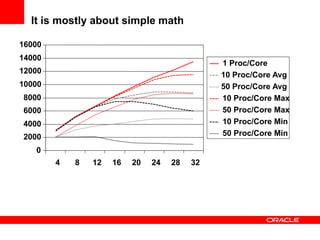
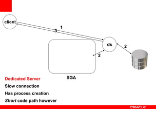
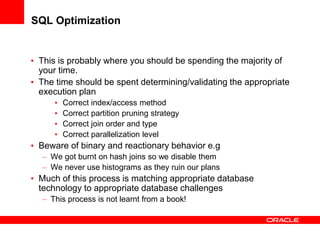
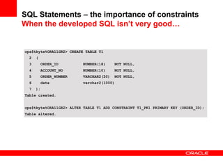
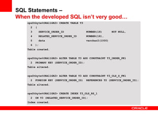
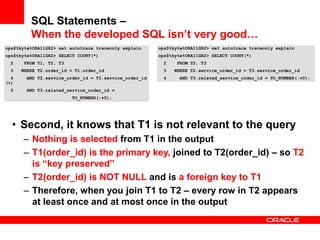
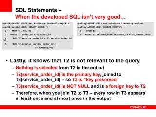
<Insert Picture Here>
Performance Summit – OLTP Performance
Andrew Holdsworth, Tom Kyte, Graham Wood
Server Technologies, Oracle Corp

Computer Science

It is mostly about simple math
0
2000
4000
6000
8000
10000
12000
14000
16000
4 8 12 16 20 24 28 32
1 Proc/Core
10 Proc/Core Avg
50 Proc/Core Avg
10 Proc/Core Max
50 Proc/Core Max
10 Proc/Core Min
50 Proc/Core Min

How much work can you do – “it depends”
Sessions & Cursors ( This slide is over 10 years old! But still true today )

Database Performance Core Principles
• To determine acceptable CPU utilization take a
probabilistic approach to the subject.
– If a CPU is 50% busy the chance of getting scheduled is 1 in 2
– If a CPU is 90% busy the chance of getting scheduled is 1 in10
• If the probabilities are used as indicator of the
predictability of user response time, then the variance
in user response time becomes noticeable at about
60-65%
• This has been observed in production and laboratory
conditions for many years.

Performance Buzz
Talk is Cheap! Performance is not!
• There is much jargon and many buzzwords used in
connection with computers and data processing.
• Do you know what they really mean?
Latency
Throughput
Response Time Efficiency
Real Time
Linear Scaling
Horizontal Scaling
Cache Efficiency
Transaction Rate

Making Connections

Three Ways to create a physical connection
• Dedicated Server
– Slow connection
– Short code path
• Shared Server
– Fast connection
– Long code path
• Database Resident Connection Pooling (DRCP)
– Fast connection
– Short code path
– Limited Availability

client
ds
1
2
2
3
SGADedicated Server
Slow connection
Has process creation
Short code path however

s001
s002
s003
s00n
…
d001
client
Request
queue
Response
queue
1
2
3
4
45
6
7
SGAShared Server
Fast connection
No process creation
Long code path however

ds
client
1
2
2
3
SGADRCP
Fast connection
No process creation
Short code path
ds
ds
.
.

ds
client
SGADRCP
Fast connection
No process creation
Short code path
ds
ds
.
.

Connection Architecture
Connection Storms
• May be caused by application servers that allow the
size of the pool of database connections to increase
rapidly when the pool is exhausted
• A connection storm may take the number of
connections from hundreds to thousands in a matter
of seconds
• The process creation and logon activity may mask the
real problem of why the connection pool was
exhausted and make debugging a longer process
• A connection storm may render the database server
unstable, unusable

The Anatomy of a Connection Storm

Non Intuitive Connection Storm
• Normally, your system ramps up to a steady state
slowly over time
• All is well
• Until a disaster strikes – and you failover
• Is your Disaster Recovery solution a failure just
waiting to happen itself
– Because you’ve “over connected” your existing data slowly
over time.

Sessions and Cursors
Are Your Clients Vulnerable to a Connection Storm?
• Do you do DR on a system with more than a few
dozen connections?
• Does your AWR or Statspack report show a logon/off
rate > 1 per second over a period of time?
• Have you set processes to a high value as a band-
aid?
• Have you even thought about it?
– How many connections do you really need?
– What could/would happen if that number is much larger than
the number of processing cores you have available?

Concurrency or Not

What is concurrency
What defines concurrency?
• Is it many connections to a database?
• Is it transactions per second?
• Is it having many active sessions?
• Is it actively doing constructive work on all of your
CPUs at the same time?

“Oracle is highly concurrent and scalable.
So you don’t have to be”
Well…

report
update
Before
Image
accurate
Person Table
The “story” (or the myth if you will)
You are concurrent without having to do anything at all…
• Updates don’t lockout
reports and reports don’t
lockout updates
• Reports see only committed
data via Multi-Versioning
• Queries yield maximum
throughput with correct
results - no waiting and no
dirty reads!
• Row locks never escalate -
the most scalable solution
available

What are major concurrency inhibitors?
• Just one – shared resources that are not shared
nicely
– Many sessions updating the same row (enqueue locks)
– Many sessions updating the same shared memory bits (latch,
mutex contention)
– Many sessions updating the same block(s) (current mode
gets – buffer busy waits)
– Many sessions trying to read the same devices (IO)
– Many sessions trying to simply be active at the same time
(CPU)
– Many sessions trying to sort at the same time
– And so on

How do you solve concurrency issues?
• There is fortunately…
– A single answer
– That answers all concurrency issues
– Absolutely and completely.
– It is….

“It Depends…”
For example…

Hot right hand side index
• Populated by sequence
(monotonically increasing
value)
• Hundreds/Thousands of
attempted concurrent inserts
• Massive contention for the
right hand side block
• How do you solve it?

SQL and Statistics

How frequently do you gather statistics
• There is fortunately…
– A single answer
– That answers all statistics gathering frequency questions
– Absolutely and completely.
– It is….
It depends of course

Statistics Frequency
• Maybe once and never again (rare)
– Global temporary tables, just get a representative sample
• Maybe every day (unlikely)
– Newly added partitions on a daily basis
– Rapidly changing data characteristics
• Maybe on a much larger period (typical)
– Most data doesn’t change that often, that massively
– Most plans won’t change with the same statistics
• Bind peeking can affect that however
• Lack of binds can affect that as well – it is the boundary
conditions we need to be concerned about

Statistics Style
• Auto Job?
• Defaults?
– Do you really want histograms?
– Do you really want silent changes?
• Estimate or Compute?
• Maybe we just set them?
• What about incremental?...

Gathering Statistics
Incremental Statistics
• One of the biggest problems with large tables is
keeping the schema statistics up to date and accurate
• To address this problem, 11.1 introduced the concept
of incremental statistics for partitioned objects
• This means that statistics are gathered for recently
modified partitions

The Concept of Synopses
• It is not possible to simply add partition statistics
together to create an up to date set of global statistics
• This is because the Number of Distinct Values (NDV)
for a partition may include values common to multiple
partitions.
• To resolve this problem, compressed representations
of the distinct values of each column are created in a
structure in the SYSAUX tablespace known as a
synopsis

Synopsis Example
Object Column Values NDV
Partition #1 1,1,3,4,5 4
Partition #2 1,2,3,4,5 5
NDV by addition WRONG 9
NDV by Synopsis CORRECT 5

SQL and Writing It

Application Design and SQL
• Relational System Design Basics
– Relational databases became so popular because they boost
application development productivity.
– Relational databases have been proven to scale with increasing data
volumes
– Relational databases provide the means to evolve and answer
multiple business questions
• This means designing a relational database
– Not a hierarchical database
– Not an object database
• This means going back to basics
– Data Modeling
– Normalization of Data
– Compromises between Logical and Physical models

SQL Statements
• It cannot be emphasized enough SQL statements
have more impact than any other performance
variable.
– Well written SQL statements that define the data to be
queried, updated etc is always the first problem. This is
clearly the responsibility of the developer or tool vendor.
– Optimizing the SQL efficiently is a mixture of the DBAs and
the Database’s responsibility
• DBA need to maintain good schema statistics to enable the
database make good cardinality estimates
• The Database needs choose efficient plans based upon good
schema statistics

SQL Design and Implementation
• Basic Checks for SQL statements and schemas
– Check for parse errors
– Validate correct join conditions specified
– Caution with implicit data type conversions
– Caution with wildcards and functions
– Caution on fuzzy joins

SQL Optimization
• This is probably where you should be spending the majority of
your time.
• The time should be spent determining/validating the appropriate
execution plan
• Correct index/access method
• Correct partition pruning strategy
• Correct join order and type
• Correct parallelization level
• Beware of binary and reactionary behavior e.g
– We got burnt on hash joins so we disable them
– We never use histograms as they ruin our plans
• Much of this process is matching appropriate database
technology to appropriate database challenges
– This process is not learnt from a book!

SQL Statements - Parsing
• Even if the SQL statement is performing well – you
might be doing extra non-necessary work
• That is called parsing
• There are three types of parsing (maybe four) in
Oracle:
– Hard parse (very very very bad)
– Soft parse (very very bad)
– Softer Soft parse (very bad)
– Absence of a parse – no parse (good)
Bind01-02-03.sql

SQL Statements – the importance of constraints
When the developed SQL isn’t very good…
ops$tkyte%ORA11GR2> CREATE TABLE T1
2 (
3 ORDER_ID NUMBER(18) NOT NULL,
4 ACCOUNT_NO NUMBER(10) NOT NULL,
5 ORDER_NUMBER VARCHAR2(20) NOT NULL,
6 data varchar2(1000)
7 );
Table created.
ops$tkyte%ORA11GR2> ALTER TABLE T1 ADD CONSTRAINT T1_PK1 PRIMARY KEY (ORDER_ID);
Table altered.

2 (
3 SERVICE_ORDER_ID NUMBER(18) NOT NULL,
4 ORDER_ID NUMBER(18) NOT NULL,
5 ORDER_STATUS_ID NUMBER(6) NOT NULL,
7 );
Table created.
ops$tkyte%ORA11GR2> ALTER TABLE T2 ADD CONSTRAINT T2_PK1
2 PRIMARY KEY (SERVICE_ORDER_ID);
Table altered.
ops$tkyte%ORA11GR2> ALTER TABLE T2 ADD CONSTRAINT T2_OSO_FK1
2 FOREIGN KEY (ORDER_ID) REFERENCES T1 (ORDER_ID);
Table altered.
SQL Statements –

2 (
3 SERVICE_ORDER_ID NUMBER(18) NOT NULL,
4 RELATED_SERVICE_ORDER_ID NUMBER(18),
6 );
Table created.
ops$tkyte%ORA11GR2> ALTER TABLE T3 ADD CONSTRAINT T3_ORDER_PK1
2 PRIMARY KEY (SERVICE_ORDER_ID);
Table altered.
ops$tkyte%ORA11GR2> ALTER TABLE T3 ADD CONSTRAINT T3_OLS_S_FK1
2 FOREIGN KEY (SERVICE_ORDER_ID) REFERENCES T2 (SERVICE_ORDER_ID);
Table altered.
ops$tkyte%ORA11GR2> CREATE INDEX T3_OLS_RS_1
2 ON T3 (RELATED_SERVICE_ORDER_ID);
Index created.
SQL Statements –

ops$tkyte%ORA10GR2> SELECT COUNT(*)
2 FROM T1, T2, T3
3 WHERE T2.order_id = T1.order_id
4 AND T2.service_order_id = T3.service_order_id (+)
5 AND T3.related_service_order_id = TO_NUMBER(:v0);
------------------------------------------------------------------------------
| Id | Operation | Name | Rows | Bytes | Cost |
------------------------------------------------------------------------------
| 0 | SELECT STATEMENT | | 1 | 65 | 2 |
| 1 | SORT AGGREGATE | | 1 | 65 | |
| 2 | NESTED LOOPS | | 1 | 65 | 2 |
| 3 | NESTED LOOPS | | 1 | 52 | 2 |
| 4 | TABLE ACCESS BY INDEX ROWID| T3 | 1 | 26 | 1 |
|* 5 | INDEX RANGE SCAN | T3_OLS_RS_1 | 1 | | 1 |
| 6 | TABLE ACCESS BY INDEX ROWID| T2 | 1 | 26 | 1 |
|* 7 | INDEX UNIQUE SCAN | T2_PK1 | 1 | | |
|* 8 | INDEX UNIQUE SCAN | T1_PK1 | 1 | 13 | |
------------------------------------------------------------------------------
2 FROM T1, T2, T3
---------------------------------------------------------------------------------
| Id | Operation | Name | Rows | Bytes | Cost (%CPU)| Time |
---------------------------------------------------------------------------------
| 0 | SELECT STATEMENT | | 1 | 26 | 1 (0)| 00:00:01 |
| 1 | SORT AGGREGATE | | 1 | 26 | | |
|* 2 | INDEX RANGE SCAN| T3_OLS_RS_1 | 1 | 26 | 1 (0)| 00:00:01 |
---------------------------------------------------------------------------------
SQL Statements –

ops$tkyte%ORA11GR2> set autotrace traceonly explain
2 FROM T1, T2, T3
4 AND T2.service_order_id = T3.service_order_id
(+)
5 AND T3.related_service_order_id =
TO_NUMBER(:v0);
• First, it knows the outer join is not necessary
– Where t2.col = t3.col(+) and t3.anything = ‘something’
– Implies the (+) is not necessary
• If the outer join ‘happened’, then t3.anything would be
NULL! And t3.anything = to_number(:v0) would never
be satisfied
2 FROM T1, T2, T3
SQL Statements –

2 FROM T1, T2, T3
(+)
TO_NUMBER(:v0);
• Second, it knows that T1 is not relevant to the query
– Nothing is selected from T1 in the output
– T1(order_id) is the primary key, joined to T2(order_id) – so T2
is “key preserved”
– T2(order_id) is NOT NULL and is a foreign key to T1
– Therefore, when you join T1 to T2 – every row in T2 appears
at least once and at most once in the output
2 FROM T2, T3
3 WHERE T2.service_order_id = T3.service_order_id
SQL Statements –

2 FROM T1, T2, T3
(+)
TO_NUMBER(:v0);
• Lastly, it knows that T2 is not relevant to the query
– Nothing is selected from T2 in the output
– T2(service_order_id) is the primary key, joined to
T3(service_order_id) – so T3 is “key preserved”
– T3(service_order_id) is NOT NULL and is a foreign key to T2
– Therefore, when you join T2 to T3 – every row in T3 appears
at least once and at most once in the output
2 FROM T3
3 WHERE T3.related_service_order_id = TO_NUMBER(:v0);
SQL Statements –

2 FROM T1, T2, T3
2 FROM T3
3 WHERE T3.related_service_order_id = TO_NUMBER(:v0);
Is the same as….
But only because of the constraints in place…
SQL Statements – the importance of constraints

SQL Statements – wrapup
• Average performance engineers very quickly learn the
following skills:
– Identification of resource intensive or poorly performing SQL
– Identification of potentially better execution plans
• Really good performance engineers are able to:
– Use cardinality estimates to identify why suboptimal execution
plans were chosen
– Take corrective action by either fixing the statistics, hand
tuning the SQL or by logging bugs
• Bad performance engineers
– Start hacking init.ora parameters on a per SQL statement
basis in random manner

SQL Statements – wrapup
• It is not just about raw SQL performance, how the
application interacts with the database counts too
– Parsing
– Array processing
• Metadata Matters
– To the optimizer, just like statistics

Application Instrumentation

Let us know who you are
• Dbms_session.set_identifier
– Audited
– Used by dbms_monitor tracking
• Dbms_application_info
– Set client info
– Set action
– Set module
– Instantly visible – gives context
• Dbms_application_info
– Set session longops

Automatic Workload Repository (AWR)
• Every N-Units of time, data is flushed from memory to
disk (a snapshot)
• You can generate reports that cover any range of time
(n-units of time at a time)
• We simply “subtract”
T1 T2 T3 T4
You can report on:
T2-T1
T3-T2
T3-T1
T4-T3
T4-T2
T4-T1
Shutdown/startup
You can report on:
T3-T2
T4-T3
T4-T2
select * from
dba_hist_snapshot;

Active Session History (ASH)
• V$ACTIVE_SESSION_HISTORY – about every second of
activity
• DBA_HIST_ACTIVE_SESS_HISTORY – every 10 seconds of
activity
– On demand flush
– When ever in memory buffer (V$) is 2/3rds full
– Retained using AWR retention policies
Point in time:
V$SESSION
V$SESSION_WAIT
SGA Circular
Buffer – sized
By CPU_COUNT
Short term memory:
V$ACTIVE_SESSION_HISTORY
Long term memory:
DBA_HIST_ACTIVE_SESS_HISTORY
Every hour or
2/3rds full in SGA

Instrumentation
• Think back to version 6… How would you tune a
system (or systems) of todays scope without it?
• The database does much of it for you
• You still have to participate a bit
– Dbms_application_info
– Dbms_session

Applications and Conversations

Real World Performance - OLTP

More Related Content

Similar to Real World Performance - OLTP

More from Connor McDonald

Recently uploaded

Real World Performance - OLTP