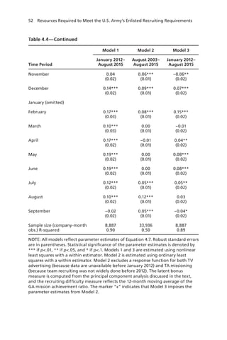
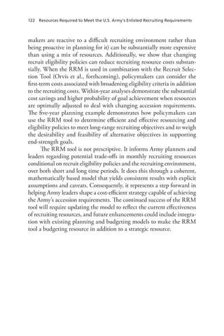
This report analyzes the resources needed to meet the U.S. Army's enlisted recruiting requirements under varying conditions and policies. It aims to optimize recruiting resource levels and assess alternative recruiting strategies to improve enlistment effectiveness. The research was conducted by the RAND Corporation and sponsored by the Army's manpower and reserve affairs department.


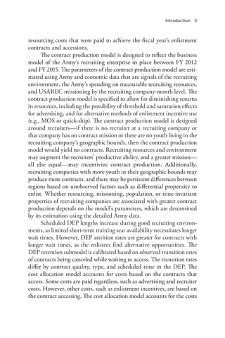
![xii Resources Required to Meet the U.S. Army’s Enlisted Recruiting Requirements
environments, it has offered additional enlistment waivers, permitted
more soldiers with prior service to enlist, and lowered educational and
test score requirements.
Understanding how recruiting resources and enlistment eligibil-
ity policies work together as a system under varying recruiting require-
ments and environments is critical for decisionmakers who want to use
their limited resources to efficiently and effectively achieve the Army’s
accession requirements. This research builds on earlier work by Defense
Manpower Data Center researchers on the effectiveness and lead times
of alternative recruiting resources in generating enlistment contracts and
accessions. The Recruiting Resource Model (RRM) developed in this
report considers the relationship among the monthly level and mix of
recruiting resources, recruit eligibility policies, accumulated contracts,
and training seat targets. It models how these factors combine to pro-
duce monthly accessions and the number of enlistment contracts at the
fiscal year’s end that are scheduled to access in the following fiscal year.
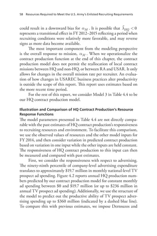
The RRM reflects the complex sequence of events leading to an
accession. It consists of a contract production submodel, a Delayed
Entry Program (DEP) retention submodel, and a cost allocation sub-
model. The contract production submodel weighs the trade-offs between
economic conditions and resources used to produce overall and high-
quality (HQ) enlistment contracts (where HQ reflects the Department
of Defense [DoD] standard of contracts where the enlistee has a formal
high school diploma and scores in the upper fiftieth percentile of the
Armed Forces Qualification Test). Based on the contract characteristics
(e.g., HQ contract, quick-ship bonus) and training seat vacancies, con-
tracts are scheduled to leave for basic training (i.e., access into the Army)
at a specific time. The time between contract and accession is known
as the time in the DEP. The DEP retention submodel captures the
probabilistic cancellation of the enlistment contract over these months.
The third submodel accounts for the resourcing costs that were paid to
achieve the fiscal year’s enlistment contracts and accessions.
The contract production model is designed to reflect the Army’s
business model—namely, team recruiting and the dual missioning of
recruiters to recruit for both the Regular (active) Army and the U.S.
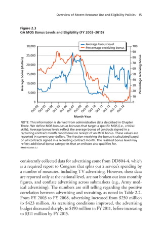
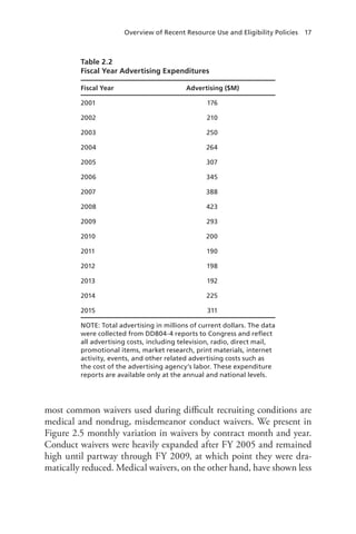
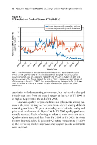
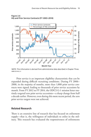
Army Reserve—of the Army’s recruiting enterprise that has been in](https://image.slidesharecdn.com/randrr2364-190327201516/85/Rand-rr2364-12-320.jpg)


![32 Resources Required to Meet the U.S. Army’s Enlisted Recruiting Requirements
by zip code based on U.S. Census population data as our main measure
of the enlistment-eligible population. Qualified military available are
defined as U.S. citizens 17–24 years of age who are eligible and available
for enlisted military service without a waiver. Ineligibility is based on
(1) medical/physical, (2) overweight, (3) mental health, (4) drugs,
(5) conduct, (6) dependents, and (7) aptitude criteria.7
Unemployment rates are measured using the Current Population
Survey, a household survey administered on a monthly basis by the U.S.
Census Bureau, and reflect the official definition of unemployment for
reporting purposes. The U.S. Bureau of Labor Statistics computes these
measures and projects county-level unemployment rates on a monthly
basis.
Remaining Technical Notes
In general, data were collected so that they would correspond to the
recruiting resources, enlistment eligibility policies, and economic con-
ditions in effect as of each calendar month from August 2002 through
September 2015. This fully covers the Army’s fiscal years from 2003
to 2016, as well as the last two months of FY 2002. However, not all
data neatly correspond to calendar months. Contract-related measures
correspond to recruiting contract months (RCMs), which typically run
from the middle of the prior month to the middle of the current month
(e.g., the May 2017 RCM runs from April 14 to May 11). Starting in
2014, USAREC changed this terminology to “phaseline”; however, we
retain the original terminology in this report. Accession-related mea-
sures correspond to recruiting ship months (RSMs). The RSM ends on
the last business day preceding the last Monday of the month, except
7 Estimates of qualified military available are calculated by applying experienced rejection
rates to military available from the geographical area using data from the National Health and
Nutrition Examination Survey, National Survey on Drug Use and Health, Joint Advertising
Market Research and Studies Youth Poll surveys, Military Entrance Processing Command
Production Applicants AFQT Score Database, Woods and Poole Economics’ Population
Estimates, and the 1997 Profile of American Youth. (See Joint Advertising Market Research
and Studies [2016].)](https://image.slidesharecdn.com/randrr2364-190327201516/85/Rand-rr2364-52-320.jpg)


![40 Resources Required to Meet the U.S. Army’s Enlisted Recruiting Requirements
. (4.2)
We can further define the structure of β( ) ( )= ⋅f UE ln UEst UE st2 ,
( )f ADst3 , ( )f ADst3 , ( )f Bonust4 , and the elements of Xst . For the
present analysis, we define β β β( )= ⋅ + ⋅ +f RE RE REt RE t RE t RE1 ,1 ,2
2
,3
β β+ ⋅ + ⋅E RE RE t RE t RE t,2
2
,3
3
so that national difficulty in recruiting can
have increasing and diminishing effects. Additionally, we define
β( ) ( )= ⋅f UE ln UEst UE st2 , consistent with the past literature on enlist-
ment contract supply. The resulting coefficient, UEβ , will represent the
percentage change response of contracts per recruiter for a given per-
centage change in unemployment.
We define f AD g ADst m
m
s t m3 0
5
,∑ ( )( ) = =
=
− , where
g ADs t m,( )− is defined as the S-curve of lag m, a functional form
introduced by Dertouzos and Garber (2003) that represents the unique
nature of advertising, where a little advertising has minimal effect, but
as marketing saturation increases and individuals are exposed to pro-
motional images of the Army, the returns to advertising increase. How-
ever, the S-curve also captures market saturation, whereby an additional
dollar spent in a market with high exposure yields no additional con-
tracts. The functional form of the S-curve is given by
+
, (4.3)
where κ θ=m
m
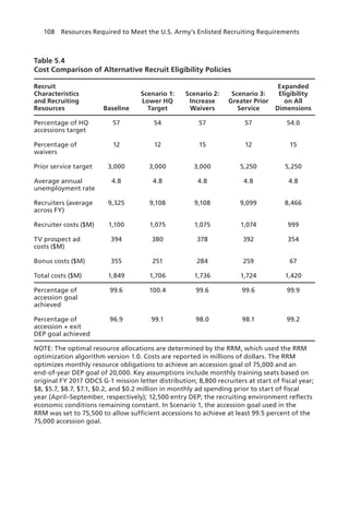
for [ ]∈m 2,5 , and the parameters κ0 , κ1, θ , and μ
are parameters to be estimated. The specification follows from Der-
touzos and Garber (2003), where the specification for κm allows for
delayed effects of TV advertising. Identification of the S-curve in Equa-
tion 4.3 relies on variation in television advertising impressions in the
recruiting company area relative to other areas. TV advertising impres-
sions vary significantly over FY 2012–2015 due in part to changes in
funds allocated to TV advertising, but also due to geographic variation
in TV viewership. To the degree that a company area is more likely to
watch TV, we can exploit the variation in dollars spent per impression](https://image.slidesharecdn.com/randrr2364-190327201516/85/Rand-rr2364-60-320.jpg)


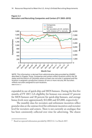
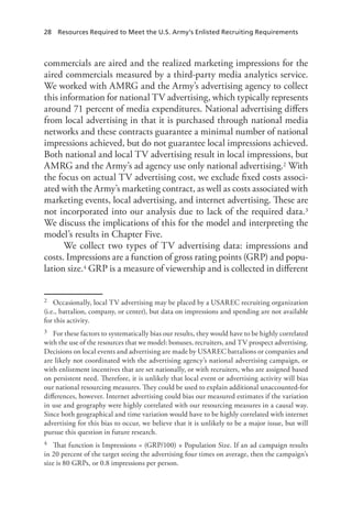
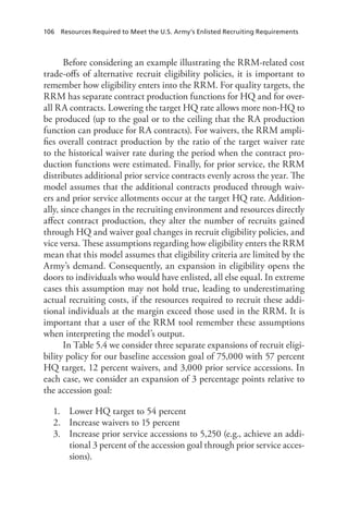
![Recruiting Resource Model 59
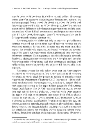
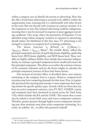
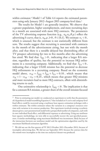
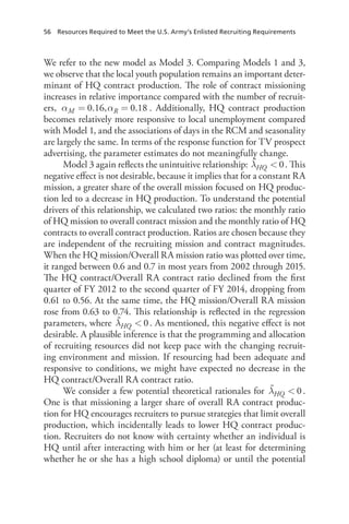
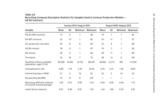
Garber’s (2003) estimates of the S-curve in 2014 dollars. We find that
the response function for TV prospect advertising indicates (1) that TV
advertising continues to be an important recruiting lever for the Army,
and (2) while TV advertising is less effective at lower expenditure levels
than in past estimates, it still reflects an S-curve that exhibits threshold
and saturation levels for TV ad spending.
Figure 4.2
HQ Contract Production Response to TV Prospect Advertising
NOTE: HQ production model estimates, both in and out of sample, correspond to HQ
contract production predictions using Model 3 of Table 4.4 and holding other
resources in FY 2014 constant. Estimates of the TV advertising response function are
from Orvis et al. (2016) and are based on Dertouzos and Garber (2003) estimates
using the Advertising Mix Test results from the mid-1980s. Orvis et al. (2016) update
this response function to 2012 based on adjustments for overall inflation (Consumer
Price Index–Urban Consumers [CPI-U]) as measured by the U.S. BLS, inflation in
advertising expenditures, and changes in the youth population level. For the
purposes of this comparison, we further inflated these values to 2014 dollars using
BLS’s CPI-U. In all cases, the monthly national TV expenditure is held constant. The
prior estimates do not distinguish between influencer and prospect TV advertising,
whereas the response function in Model 3 of Table 4.4 is limited to only TV prospect
advertising (i.e., advertising impressions for males aged 18–24).
RAND RR2364A-4.2
16,000
14,000
12,000
10,000
8,000
6,000
4,000
2,000
0
0 50 100 150 200 250 300 350
HQ contract production
model (within sample)
HQ contract production
model (out of sample)
Prior estimate based on
1980’s data
HQenlistmentcontracts
Annual spending TV advertising ($M)](https://image.slidesharecdn.com/randrr2364-190327201516/85/Rand-rr2364-79-320.jpg)

![62 Resources Required to Meet the U.S. Army’s Enlisted Recruiting Requirements
fixed eligibility level, was made as part of the Enlistment Bonus Experi-
ment that took place in the early 1980s (Polich, Dertouzos, and Press,
1986). In this case, the authors found a bonus elasticity of between
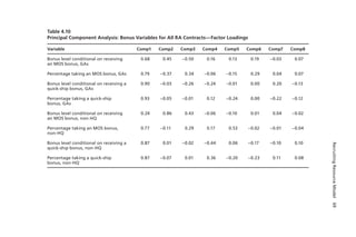
0.07 and 0.08. Our estimates are reported in Tables 4.6 and 4.7. The
estimates in Table 4.6 reflect the expansion of a $12,000 MOS or quick-
ship bonus to a growing pool of eligible training seats for which a poten-
tial enlistee may choose to sign up. Quick-ship bonuses are estimated
to be slightly more productive than MOS bonuses for HQ contracts.
Estimated elasticities range from 0.02 to 0.11. Both bonus types exhibit
diminishing returns. When MOS and quick-ship bonuses are increased
in tandem, the point of diminishing returns occurs sooner due to sub-
stitutability between the bonus types.
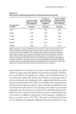
Table 4.7 presents similar measures of the HQ contract produc-
tion’s response to increases in enlistment bonus levels. We find that HQ
contract production increases with increasing bonus levels and that,
similar to expanding eligibility, increasing bonus levels for both bonus
types exhibits increasing responsiveness at low levels of bonuses, but
diminishing at high levels. The results in Table 4.7 are most analogous
to those in the Enlistment Bonus Experiment. The experiment fixed the
MOSs eligible for bonuses and allowed the bonus level to differ between
specific recruiting areas and length of enlistment contract. In the Enlist-
ment Bonus Experiment, the control group was offered a $5,000 MOS
bonus (equivalent to about $12,000 in today’s dollars) and the first
experimental group was offered an $8,000 bonus for the same MOS
and same four-year contract length (equivalent to about $20,000). The
second experimental group was offered either an $8,000 bonus for the
same MOS and same four-year contract length or a $4,000 bonus for a
three-year contract length for the same MOS. HQ enlistments into the
eligible MOS represented just under 30 percent of all HQ enlistments
during the baseline (preceding) year (see Table 3 of Polich, Dertouzos,
and Press [1986]). Our estimates in Table 4.7 of $12,000 and $20,000,
respectively, suggest that our measured bonus elasticity is greater than
earlier estimates, but in the same relative region as the Enlistment Bonus
Experiment and past measures of bonus responsiveness.
These measures of bonus elasticity are closely related to the con-
cept of economic rent, which in the present context means the fraction](https://image.slidesharecdn.com/randrr2364-190327201516/85/Rand-rr2364-82-320.jpg)


![Recruiting Resource Model 79
both HQ and non-HQ production proportionately. If the target waiver
rate exceeds the historical waiver rate, the number of contracts produced
increases; if the target waiver rate is below the historical waiver rate, it
will reduce the number of contracts produced.
Finally, since the contract production models reflect NPS pro-
duction, prior service contracts are produced based on target prior ser-
vice accessions and these contracts are uniformly distributed across the
RCM within the fiscal year. The target HQ contracting rate determines
the proportion of HQ versus non-HQ prior service contracts.
The contract production model takes the following as inputs:
resourcing levels, eligibility policy (i.e., target HQ percentage, waiver
rates, prior service accession targets), recruiting environment (i.e.,
unemployment rate and the recruiting difficulty measure from Wenger
et al. [forthcoming]), and the observed distribution of recruiting compa-
nies, recruiters, advertising exposure (the ratio of company-area impres-
sions relative to national impressions), and local unemployment rates
observed in FY 2014. The contract production model’s outputs are the
number of contracts produced by type (i.e., HQ or non-HQ) and with
or without a quick-ship bonus.
DEP Retention Model
Once contracts are produced by the contract production function, they
are assigned a DEP length based on existing training seat vacancies.
The distribution of training seats reflects the distribution of target HQ
contracts and is scaled to reflect the accession goals. While the enlistee
is waiting to access, he or she has a probability of canceling the enlist-
rate is already reflected in the contract production function and that an expansion or
contraction of the waiver rate has an effect on contract production that is indepen-
dent of recruiting resources. In essence, we are assuming these contracts are demand
constrained—they are ready and willing to enlist only if the Army accepts them. In
extreme cases, for examples beyond waiver rates observed in recent history (a bit over
20 percent for our sample period), this assumption may not be valid. If the contracts
produced through waivers were not demand constrained, then the contract produc-
tion function would predict more contracts are produced than in reality.](https://image.slidesharecdn.com/randrr2364-190327201516/85/Rand-rr2364-99-320.jpg)


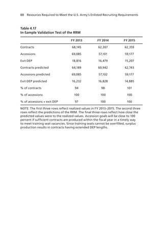
![Recruiting Resource Model 85
on Orvis et al. [2016]). We use FY 2014 contract cancellation rates
based on months scheduled to be in the DEP to impute a distribution
for how many months the contracts were originally scheduled for. For
example, for GA contracts with one month remaining in the DEP at
the beginning of the fiscal year, we impute a value for what fraction
of those contracts had a DEP length of one month, two months, and
so on. Based on the results in Table 4.16, if an entry pool is composed
more heavily of contracts signed with longer DEP lengths, then more
contracts are likely to be canceled in the current fiscal year.
The DEP retention model takes the following as inputs: the output
of the contract production model; a user-specified training seat dis-
tribution, accession goal, target HQ accession percentage, and entry
pool size; and the calibrated measures described above using observed
FY 2014’s distribution of DEP length and DEP attrition rates. Varia-
tion in external economic conditions influences DEP retention because
higher rates of contract production during particularly good recruiting
conditions result in longer DEP lengths (and hence greater attrition).
The DEP retention model’s outputs are accessions by month of the
fiscal year and by type (e.g., HQ or non-HQ), the number of contracts
in the DEP for the next year (i.e., entry pool for next fiscal year), and
the number of eventual accessions by type for contracts signed in the
current fiscal year.
Cost Allocation Model
Resourcing costs are allocated to the month a resource is used. For
advertising, this corresponds to the month the advertising originally
airs. For recruiters, we follow HQDA guidance and allocate a constant
recruiter annual cost of $118,000 per year, or about $9,800 per month.14
The recruiter cost reflects the number of recruiters on production in a
month times the cost per recruiter. Finally, bonus costs reported in the
model reflect obligations made during the fiscal year. These costs are
14 This value was provided to RAND by HQDA.](https://image.slidesharecdn.com/randrr2364-190327201516/85/Rand-rr2364-105-320.jpg)


![123
APPENDIX A
Example of Changes in Production Elasticities
This appendix deals with a technical issue related to how measured
elasticities on a production curve that exhibit diminishing or constant
returns to an input could result in increasing or increasing then decreas-
ing elasticities over a range of inputs. The source of this result is related
to the relative change in the input compared with the output. Consider
the two illustrative examples in Table A.1.
The first example reflects constant returns of output Y from a fixed
increment of input X. The second example reflects diminishing returns
of output Y from a fixed increment of input X. Recall that an elasticity is
calculated as the percentage change in output Y divided by a percentage
change in input X. The point elasticity at a point midway between input
X1 and X2 (e.g., calculating the elasticity at 0.1 [midpoint] would use
=X 01 and =X 0.22 ) is calculated numerically using the following
midpoint formula:
Elasticity =
Y2−Y1
Y2 +Y1( )/ 2
⎛
⎝
⎜⎜⎜⎜
⎞
⎠
⎟⎟⎟⎟
X2− X1
X2 + X1( )/ 2
⎛
⎝
⎜⎜⎜⎜
⎞
⎠
⎟⎟⎟⎟
where Y1 corresponds to the output from X1 , and Y2 corresponds
to the output from X2 , all else equal. In both of these examples, the
output Y starts from a relatively high level, suggesting that, while X
has a positive impact in producing Y, it represents a small fraction of
overall production. Consequently, as input X increases, the percentage](https://image.slidesharecdn.com/randrr2364-190327201516/85/Rand-rr2364-143-320.jpg)


![[Full Report] Barriers and Opportunities at the Base of the Pyramid - The Rol...](https://cdn.slidesharecdn.com/ss_thumbnails/undp-osd-barriersandopportunitiesbopfullreportweb-140822084014-phpapp01-thumbnail.jpg?width=640&height=640&fit=bounds)


![Shrm Achieve Future Changes Workforce 120925153125 Phpapp01[1]](https://cdn.slidesharecdn.com/ss_thumbnails/shrmachievefuturechangesworkforce120925153125phpapp011-13486947202988-phpapp01-120926162650-phpapp01-thumbnail.jpg?width=640&height=640&fit=bounds)


