Rainfallrunoff Modelling The Primer 2nd Edition Keith Bevenauth

Rainfallrunoff Modelling The Primer 2nd Edition
Keith Bevenauth download
https://ebookbell.com/product/rainfallrunoff-modelling-the-
primer-2nd-edition-keith-bevenauth-4311278
Explore and download more ebooks at ebookbell.com

Here are some recommended products that we believe you will be
interested in. You can click the link to download.
Rainfallrunoff Modelling The Primer 1st Edition Keith J Beven
https://ebookbell.com/product/rainfallrunoff-modelling-the-primer-1st-
edition-keith-j-beven-2265224
Use Of Metaheuristic Techniques In Rainfallrunoff Modelling Kwokwing
Chau
https://ebookbell.com/product/use-of-metaheuristic-techniques-in-
rainfallrunoff-modelling-kwokwing-chau-54691550
Kinematicwave Rainfallrunoff Formulas 1st Edition Tommy S W Wong
https://ebookbell.com/product/kinematicwave-rainfallrunoff-
formulas-1st-edition-tommy-s-w-wong-2379718
Possibility Of Using Selected Rainfallrunoff Models For Determining
The Design Hydrograph In Mountainous Catchments A Case Study In Poland
Dariusz Myski
https://ebookbell.com/product/possibility-of-using-selected-
rainfallrunoff-models-for-determining-the-design-hydrograph-in-
mountainous-catchments-a-case-study-in-poland-dariusz-myski-11054588

Effect Of Rainfall Runoff And Infiltration Processes On The Stability
Of Footslopes Hungen Chen
https://ebookbell.com/product/effect-of-rainfall-runoff-and-
infiltration-processes-on-the-stability-of-footslopes-hungen-
chen-10974280
Rainfall Modeling Measurement And Applications 1st Edition Renato
Morbidelli Editor
https://ebookbell.com/product/rainfall-modeling-measurement-and-
applications-1st-edition-renato-morbidelli-editor-46412446
Rainfall The Anrodnes Chronicles Book 4 J C Owens
https://ebookbell.com/product/rainfall-the-anrodnes-chronicles-
book-4-j-c-owens-49265280
Rainfall Infiltration In Unsaturated Soil Slope Failure Lizhou Wu
https://ebookbell.com/product/rainfall-infiltration-in-unsaturated-
soil-slope-failure-lizhou-wu-50401638
Rainfall Behavior Forecasting And Distribution 1st Edition Olga E
Martn Tricia M Roberts
https://ebookbell.com/product/rainfall-behavior-forecasting-and-
distribution-1st-edition-olga-e-martn-tricia-m-roberts-51369016

Rainfall-Runoff Modelling
The Primer
SECOND EDITION
Keith Beven
Lancaster University, UK

This edition first published 2012 © 2012 by John Wiley & Sons, Ltd
Wiley-Blackwell is an imprint of John Wiley & Sons, formed by the merger of Wiley’s global Scientific, Technical
and Medical business with Blackwell Publishing.
Registered office: John Wiley & Sons, Ltd, The Atrium, Southern Gate, Chichester, West Sussex, PO19 8SQ, UK
Editorial offices: 9600 Garsington Road, Oxford, OX4 2DQ, UK
The Atrium, Southern Gate, Chichester, West Sussex, PO19 8SQ, UK
111 River Street, Hoboken, NJ 07030-5774, USA
For details of our global editorial offices, for customer services and for information about how to apply for
permission to reuse the copyright material in this book please see our website at www.wiley.com/wiley-blackwell.
The right of the author to be identified as the author of this work has been asserted in accordance with the UK
Copyright, Designs and Patents Act 1988.
All rights reserved. No part of this publication may be reproduced, stored in a retrieval system, or transmitted, in any
form or by any means, electronic, mechanical, photocopying, recording or otherwise, except as permitted by the UK
Copyright, Designs and Patents Act 1988, without the prior permission of the publisher.
Designations used by companies to distinguish their products are often claimed as trademarks. All brand names and
product names used in this book are trade names, service marks, trademarks or registered trademarks of their
respective owners. The publisher is not associated with any product or vendor mentioned in this book. This
publication is designed to provide accurate and authoritative information in regard to the subject matter covered. It is
sold on the understanding that the publisher is not engaged in rendering professional services. If professional advice
or other expert assistance is required, the services of a competent professional should be sought.
Library of Congress Cataloging-in-Publication Data
Beven, K. J.
Rainfall-runoff modelling : the primer / Keith Beven. – 2nd ed.
p. cm.
Includes bibliographical references and index.
ISBN 978-0-470-71459-1 (cloth)
1. Runoff–Mathematical models. 2. Rain and rainfall–Mathematical models.
I. Title.
GB980.B48 2011
551.488–dc23
2011028243
A catalogue record for this book is available from the British Library.
Wiley also publishes its books in a variety of electronic formats. Some content that appears in print may not be
available in electronic books.
Set in 10/12pt Times by Thomson Digital, Noida, India
First Impression 2012

For the next generation of hydrological modellers

Contents
Preface to the Second Edition xiii
About the Author xvii
List of Figures xix
1 Down to Basics: Runoff Processes and the Modelling Process 1
1.1 Why Model? 1
1.2 How to Use This Book 3
1.3 The Modelling Process 3
1.4 Perceptual Models of Catchment Hydrology 6
1.5 Flow Processes and Geochemical Characteristics 13
1.6 Runoff Generation and Runoff Routing 15
1.7 The Problem of Choosing a Conceptual Model 16
1.8 Model Calibration and Validation Issues 18
1.9 Key Points from Chapter 1 21
Box 1.1 The Legacy of Robert Elmer Horton (1875–1945) 22
2 Evolution of Rainfall–Runoff Models: Survival of the Fittest? 25
2.1 The Starting Point: The Rational Method 25
2.2 Practical Prediction: Runoff Coefﬁcients and Time Transformations 26
2.3 Variations on the Unit Hydrograph 33
2.4 Early Digital Computer Models: The Stanford Watershed Model and
Its Descendants 36
2.5 Distributed Process Description Based Models 40
2.6 Simpliﬁed Distributed Models Based on Distribution Functions 42
2.7 Recent Developments: What is the Current State of the Art? 43
2.8 Where to Find More on the History and Variety of Rainfall–Runoff Models 43
Box 2.1 Linearity, Nonlinearity and Nonstationarity 45
Box 2.2 The Xinanjiang, ARNO or VIC Model 46
Box 2.3 Control Volumes and Differential Equations 49

viii Contents
3 Data for Rainfall–Runoff Modelling 51
3.1 Rainfall Data 51
3.2 Discharge Data 55
3.3 Meteorological Data and the Estimation of Interception and Evapotranspiration 56
3.4 Meteorological Data and The Estimation of Snowmelt 60
3.5 Distributing Meteorological Data within a Catchment 61
3.6 Other Hydrological Variables 61
3.7 Digital Elevation Data 61
3.8 Geographical Information and Data Management Systems 66
3.9 Remote-sensing Data 67
3.10 Tracer Data for Understanding Catchment Responses 69
3.11 Linking Model Components and Data Series 70
Box 3.1 The Penman–Monteith Combination Equation for Estimating
Evapotranspiration Rates 72
Box 3.2 Estimating Interception Losses 76
Box 3.3 Estimating Snowmelt by the Degree-Day Method 79
4 Predicting Hydrographs Using Models Based on Data 83
4.1 Data Availability and Empirical Modelling 83
4.2 Doing Hydrology Backwards 84
4.3 Transfer Function Models 87
4.4 Case Study: DBM Modelling of the CI6 Catchment at Llyn Briane, Wales 93
4.5 Physical Derivation of Transfer Functions 95
4.6 Other Methods of Developing Inductive Rainfall–Runoff Models from Observations 99
Box 4.1 Linear Transfer Function Models 107
Box 4.2 Use of Transfer Functions to Infer Effective Rainfalls 112
Box 4.3 Time Variable Estimation of Transfer Function Parameters and Derivation
of Catchment Nonlinearity 113
5 Predicting Hydrographs Using Distributed Models Based on Process Descriptions 119
5.1 The Physical Basis of Distributed Models 119
5.2 Physically Based Rainfall–Runoff Models at the Catchment Scale 128
5.3 Case Study: Modelling Flow Processes at Reynolds Creek, Idaho 135
5.4 Case Study: Blind Validation Test of the SHE Model on the Slapton Wood
Catchment 138
5.5 Simpliﬁed Distributed Models 140
5.6 Case Study: Distributed Modelling of Runoff Generation at Walnut Gulch, Arizona 148
5.7 Case Study: Modelling the R-5 Catchment at Chickasha, Oklahoma 151
5.8 Good Practice in the Application of Distributed Models 154
5.9 Discussion of Distributed Models Based on Continuum Differential Equations 155
Box 5.1 Descriptive Equations for Subsurface Flows 158

Contents ix
Box 5.2 Estimating Infiltration Rates at the Soil Surface 160
Box 5.3 Solution of Partial Differential Equations: Some Basic Concepts 166
Box 5.4 Soil Moisture Characteristic Functions for Use in the Richards Equation 171
Box 5.5 Pedotransfer Functions 175
Box 5.6 Descriptive Equations for Surface Flows 177
Box 5.7 Derivation of the Kinematic Wave Equation 181
6 Hydrological Similarity, Distribution Functions and Semi-Distributed
Rainfall–Runoff Models 185
6.1 Hydrological Similarity and Hydrological Response Units 185
6.2 The Probability Distributed Moisture (PDM) and Grid to Grid (G2G) Models 187
6.3 TOPMODEL 190
6.4 Case Study: Application of TOPMODEL to the Saeternbekken Catchment, Norway 198
6.5 TOPKAPI 203
6.6 Semi-Distributed Hydrological Response Unit (HRU) Models 204
6.7 Some Comments on the HRU Approach 207
Box 6.1 The Theory Underlying TOPMODEL 210
Box 6.2 The Soil and Water Assessment Tool (SWAT) Model 219
Box 6.3 The SCS Curve Number Model Revisited 224
7 Parameter Estimation and Predictive Uncertainty 231
7.1 Model Calibration or Conditioning 231
7.2 Parameter Response Surfaces and Sensitivity Analysis 233
7.3 Performance Measures and Likelihood Measures 239
7.4 Automatic Optimisation Techniques 241
7.5 Recognising Uncertainty in Models and Data: Forward Uncertainty Estimation 243
7.6 Types of Uncertainty Interval 244
7.7 Model Calibration Using Bayesian Statistical Methods 245
7.8 Dealing with Input Uncertainty in a Bayesian Framework 247
7.9 Model Calibration Using Set Theoretic Methods 249
7.10 Recognising Equifinality: The GLUE Method 252
7.11 Case Study: An Application of the GLUE Methodology in Modelling the
Saeternbekken MINIFELT Catchment, Norway 258
7.12 Case Study: Application of GLUE Limits of Acceptability Approach to Evaluation
in Modelling the Brue Catchment, Somerset, England 261
7.13 Other Applications of GLUE in Rainfall–Runoff Modelling 265
7.14 Comparison of GLUE and Bayesian Approaches to Uncertainty Estimation 266
7.15 Predictive Uncertainty, Risk and Decisions 267
7.16 Dynamic Parameters and Model Structural Error 268
7.17 Quality Control and Disinformation in Rainfall–Runoff Modelling 269
7.18 The Value of Data in Model Conditioning 274
Box 7.1 Likelihood Measures for use in Evaluating Models 276
Box 7.2 Combining Likelihood Measures 283
Box 7.3 Defining the Shape of a Response or Likelihood Surface 284

x Contents
8 Beyond the Primer: Models for Changing Risk 289
8.1 The Role of Rainfall–Runoff Models in Managing Future Risk 289
8.2 Short-Term Future Risk: Flood Forecasting 290
8.3 Data Requirements for Flood Forecasting 291
8.4 Rainfall–Runoff Modelling for Flood Forecasting 293
8.5 Case Study: Flood Forecasting in the River Eden Catchment, Cumbria, England 297
8.6 Rainfall–Runoff Modelling for Flood Frequency Estimation 299
8.7 Case Study: Modelling the Flood Frequency Characteristics on the Skalka Catchment,
Czech Republic 302
8.8 Changing Risk: Catchment Change 305
8.9 Changing Risk: Climate Change 307
Box 8.1 Adaptive Gain Parameter Estimation for Real-Time Forecasting 311
9 Beyond the Primer: Next Generation Hydrological Models 313
9.1 Why are New Modelling Techniques Needed? 313
9.2 Representative Elementary Watershed Concepts 315
9.3 How are the REW Concepts Different from Other Hydrological Models? 318
9.4 Implementation of the REW Concepts 318
9.5 Inferring Scale-Dependent Hysteresis from Simpliﬁed Hydrological Theory 320
9.6 Representing Water Fluxes by Particle Tracking 321
9.7 Catchments as Complex Adaptive Systems 324
9.8 Optimality Constraints on Hydrological Responses 325
10 Beyond the Primer: Predictions in Ungauged Basins 329
10.1 The Ungauged Catchment Challenge 329
10.2 The PUB Initiative 330
10.3 The MOPEX Initiative 331
10.4 Ways of Making Predictions in Ungauged Basins 331
10.5 PUB as a Learning Process 332
10.6 Regression of Model Parameters Against Catchment Characteristics 333
10.7 Donor Catchment and Pooling Group Methods 335
10.8 Direct Estimation of Hydrograph Characteristics for Constraining Model Parameters 336
10.9 Comparing Regionalisation Methods for Model Parameters 338
10.10 HRUs and LSPs as Models of Ungauged Basins 339
10.11 Gauging the Ungauged Basin 339
11 Beyond the Primer: Water Sources and Residence Times in Catchments 343
11.1 Natural and Artiﬁcial Tracers 343
11.2 Advection and Dispersion in the Catchment System 345
11.3 Simple Mixing Models 346
11.4 Assessing Spatial Patterns of Incremental Discharge 347
11.5 End Member Mixing Analysis (EMMA) 347

Contents xi
11.6 On the Implications of Tracer Information for Hydrological Processes 348
11.7 Case Study: End Member Mixing with Routing 349
11.8 Residence Time Distribution Models 353
11.9 Case Study: Predicting Tracer Transport at the Gårdsjön Catchment, Sweden 357
11.10 Implications for Water Quality Models 359
Box 11.1 Representing Advection and Dispersion 361
Box 11.2 Analysing Residence Times in Catchment Systems 365
12 Beyond the Primer: Hypotheses, Measurements and Models of Everywhere 369
12.1 Model Choice in Rainfall–Runoff Modelling as Hypothesis Testing 369
12.2 The Value of Prior Information 371
12.3 Models as Hypotheses 372
12.4 Models of Everywhere 374
12.5 Guidelines for Good Practice 375
12.6 Models of Everywhere and Stakeholder Involvement 376
12.7 Models of Everywhere and Information 377
12.8 Some Final Questions 378
Appendix A Web Resources for Software and Data 381
Appendix B Glossary of Terms 387
References 397
Index 449

Preface to the Second Edition
Models are undeniably beautiful, and a man may justly be proud to be seen in their company.
But they may have their hidden vices. The question is, after all, not only whether they are
good to look at, but whether we can live happily with them.
A. Kaplan, 1964
One is left with the view that the state of water resources modelling is like an economy
subject to inflation – that there are too many models chasing (as yet) too few applications;
that there are too many modellers chasing too few ideas; and that the response is to print
ever-increasing quantities of paper, thereby devaluing the currency, vast amounts of which
must be tendered by water resource modellers in exchange for their continued employment.
Robin Clarke, 1974
It is already (somewhat surprisingly) 10 years since the first edition of this book appeared. It is (even
more surprisingly) 40 years since I started my own research career on rainfall–runoff modelling. That
is 10 years of increasing computer power and software development in all sorts of domains, some of
which has been applied to the problem of rainfall–runoff modelling, and 40 years since I started to try to
understand some of the difficulties of representing hydrological processes and identifying rainfall–runoff
model parameters. This new edition reflects some of the developments in rainfall–runoff modelling since
the first edition, but also the fact that many of the problems of rainfall–runoff modelling have not really
changed in that time. I have also had to accept the fact that it is now absolutely impossible for one person
to follow all the literature relevant to rainfall–runoff modelling. To those model developers who will be
disappointed that their model does not get enough space in this edition, or even more disappointed that
it does not appear at all, I can only offer my apologies. This is necessarily a personal perspective on the
subject matter and, given the time constraints of producing this edition, I may well have missed some
important papers (or even, given this aging brain, overlooked some that I found interesting at the time!).
It has been a source of some satisfaction that many people have told me that the first edition of
this book has been very useful to them in either teaching or starting to learn rainfall–runoff modelling
(even Anna, who by a strange quirk of fate did, in the end, actually have to make use of it in her
MSc course), but it is always a bit daunting to go back to something that was written a decade ago to
see just how much has survived the test of time and how much has been superseded by the wealth of
research that has been funded and published since, even if this has continued to involve the printing of
ever-increasing quantities of paper (over 30 years after Robin Clarke’s remarks above). It has actually
been a very interesting decade for research in rainfall–runoff modelling that has seen the Prediction in
Ungauged Basins (PUB) initiative of the International Association of Hydrological Scientists (IAHS), the

xiv Preface
implementation of the Representative Elementary Watershed (REW) concepts, the improvement of land
surface parameterisations as boundary conditions for atmospheric circulation models, the much more
widespread use of distributed conceptual models encouraged by the availability of freeware software
such as SWAT, developments in data assimilation for forecasting, the greater understanding of problems
of uncertainty in model calibration and validation, and other advances. I have also taken the opportunity
to add some material that received less attention in the first edition, particularly where there has been
some interesting work done in the last decade. There are new chapters on regionalisation methods, on
modelling residence times of water in catchments, and on the next generation of hydrological models.
Going back to the original final paragraph of the 1st edition, I suggested that:
The future in rainfall–runoff modelling is therefore one of uncertainty: but this then implies
a further question as to how best to constrain that uncertainty. The obvious answer is by
conditioning on data, making special measurements where time, money and the importance
of a particular application allow. It is entirely appropriate that this introduction to available
rainfall–runoff modelling techniques should end with this focus on the value of field data.
This has not changed in the last 10 years. The development, testing and application of rainfall–runoff
models is still strongly constrained by the availability of data for model inputs, boundary conditions and
parameter values. There are still important issues of how to estimate the resulting uncertainties in model
predictions. There are still important issues of scale and commensurability between observed and model
variables. There have certainly been important and interesting advances in rainfall–runoff modelling
techniques, but we are still very dependent on the quantity and quality of available data. Uncertainty
estimation is now used much more widely than a decade ago, but it should not be the end point of an
analysis. Instead, it should always leave the question: what knowledge or data are required to constrain
the uncertainty further?
In fact, one of the reasons why there has been little in really fundamental advances over the last decade
is that hydrology remains constrained by the measurement techniques available to it. This may seem
surprising in the era of remote sensing and pervasive wireless networking. However, it has generally
proven difficult to derive useful hydrological information from this wealth of data that has become (or is
becoming) available. Certainly none of the developments in field measurements have yet really changed
the ways in which rainfall–runoff modelling is actually done. At the end of this edition, I will again look
forward to when and how this might be the case.
I do believe that the nature of hydrological modelling is going to change in the near future. In part, this
is the result of increased availability of computer power (I do not look back to the days when my PhD
model was physically two boxes of punched cards with any nostalgia . . . programming is so much easier
now, although using cards meant that we were very much more careful about checking programs before
submitting them and old cards were really good for making to-do lists!). In part, it will be the result of
the need to cover a range of scales and coupled processes to satisfy the needs of integrated catchment
management. In part, it will be the result of increased involvement of local stakeholders in the formulation
and evaluation of models used in decision making. In part, it will be the desire to try to constrain the
uncertainty in local predictions to satisfy local stakeholders. The result will be the implementation of
“models of everywhere” as a learning and hypothesis testing process. I very much hope that this will give
some real impetus to improving hydrological science and practice akin to a revolution in the ways that
we do things. Perhaps in another decade, we will start to see the benefits of this revolution.
It has been good to work with a special group of doctoral students, post-docs, colleagues and collabora-
tors in the last 10 years in trying to further the development of rainfall–runoff modelling and uncertainty
estimation methods. I would particularly like to mention Peter Young, Andy Binley, Kathy Bashford, Paul
Bates, Sarka Blazkova, Rich Brazier, Wouter Buytaert, Flavie Cernesson, Hyung Tae Choi, Jess Davies,
Jan Feyen, Luc Feyen, Jim Freer, Francesc Gallart, Ion Iorgulescu, Christophe Joerin, John Juston, Rob

Preface xv
Lamb, Dave Leedal, Liu Yangli, Hilary McMillan, Steve Mitchell, Mo Xingguo, Charles Obled, Trevor
Page, Florian Pappenberger, Renata Romanowicz, Jan Seibert, Daniel Sempere, Paul Smith, Jonathan
Tawn, Jutta Thielen, Raul Vazquez, Ida Westerberg, Philip Younger and Massimiliano Zappa. Many oth-
ers have made comments on the first edition or have contributed to valuable discussions and debates that
have helped me think about the nature of the modelling process, including Kevin Bishop, John Ewen,
Peter Germann, Sven Halldin, Jim Hall, Hoshin Gupta, Dmiti Kavetski, Jim Kirchner, Mike Kirkby, Keith
Loague, Jeff McDonnell, Alberto Montanari, Enda O’Connell, Geoff Pegram, Laurent Pfister, Andrea
Rinaldo, Allan Rodhe, Jonty Rougier, Murugesu Sivapalan, Bertina Schaefli, Stan Schymanski, Lenny
Smith, Ezio Todini, Thorsten Wagener, and Erwin Zehe. We have not always agreed about an appropriate
strategy but long may the (sometimes vigorous) debates continue. There is still much more to be done,
especially to help guide the next generation of hydrologists in the right direction . . . !
Keith Beven
Outhgill, Lancaster, Fribourg and Uppsala, 2010–11

About the Author
The author programmed his ﬁrst rainfall–runoff model in 1970, trying to predict the runoff genera-
tion processes on Exmoor during the Lynmouth ﬂood. Since then, he has been involved in many of
the major rainfall–runoff modelling innovations including TOPMODEL, the Système Hydrologique
Européen (SHE) model, the Institute of Hydrology Distributed Model (IHDM) and data-based mecha-
nistic (DBM) modelling methodology. He has published over 350 papers and a number of other books.
He was awarded the IAHS/WMO/UNESCO International Hydrology Prize in 2009; the EGU Dalton
Medal in 2004; and the AGU Horton Award in 1991. He has worked at Lancaster University since 1985
and currently has visiting positions at Uppsala University and the London School of Economics.

List of Figures
1.1 Staining by dye after infiltration at the soil profile scale in a forested catchment in
the Chilean Andes (from Blume et al., 2009). 2
1.2 A schematic outline of the steps in the modelling process. 4
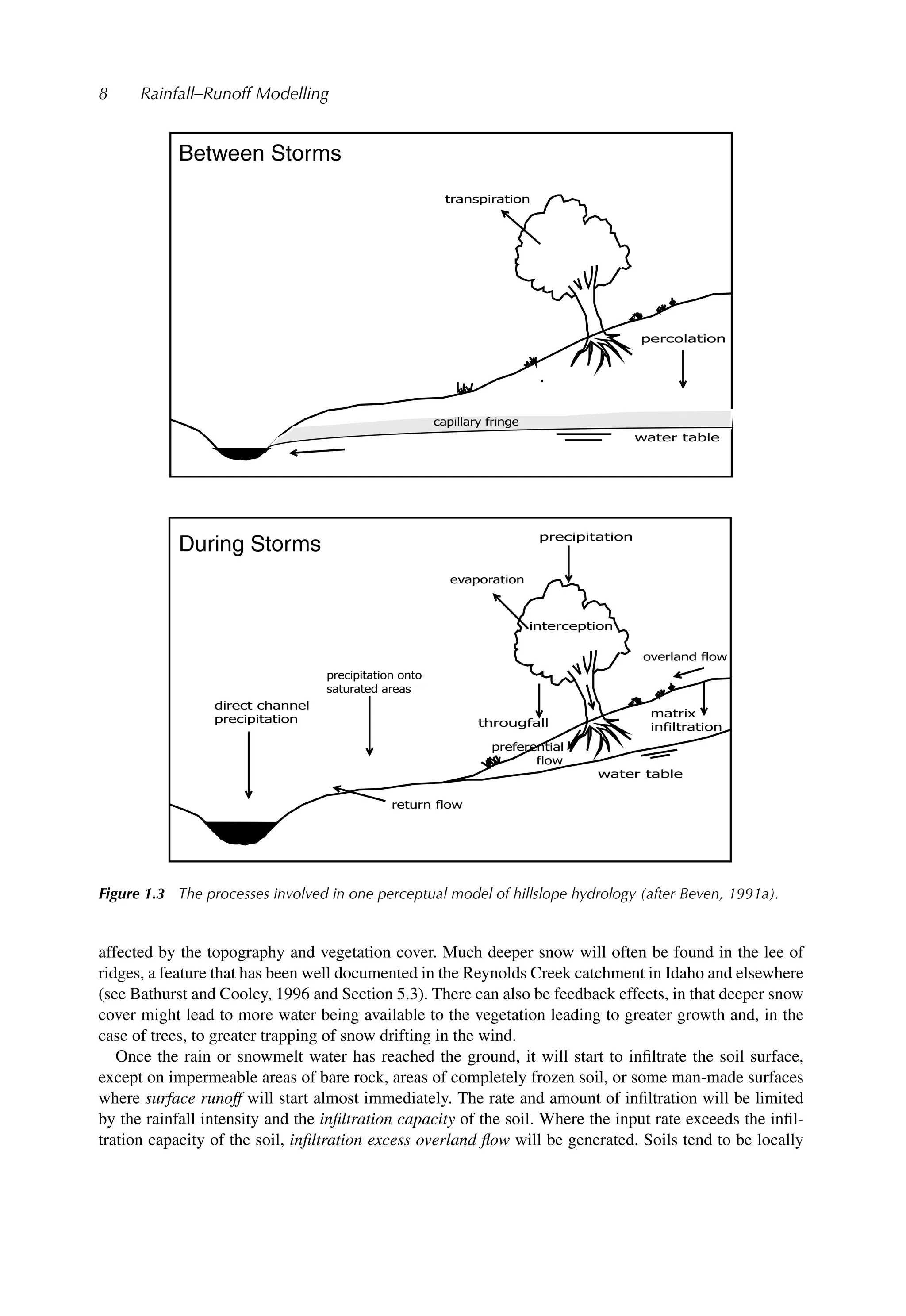
1.3 The processes involved in one perceptual model of hillslope hydrology (after
Beven, 1991a). 8
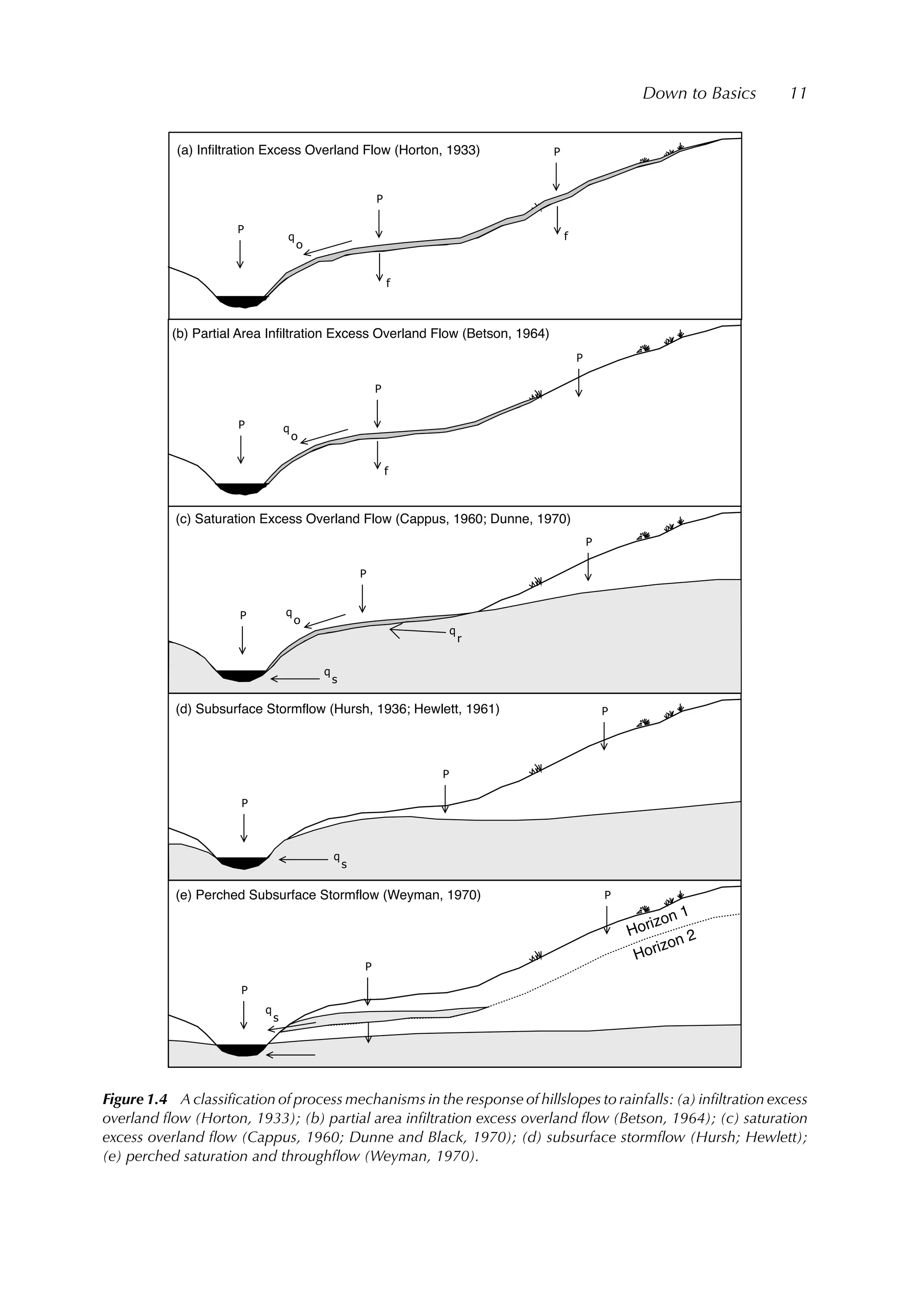
1.4 A classification of process mechanisms in the response of hillslopes to rainfalls: (a)
infiltration excess overland flow (Horton, 1933); (b) partial area infiltration excess
overland flow (Betson, 1964); (c) saturation excess overland flow (Cappus, 1960;
Dunne and Black, 1970); (d) subsurface stormflow (Hursh; Hewlett); E. perched
saturation and throughflow (Weyman, 1970). 11
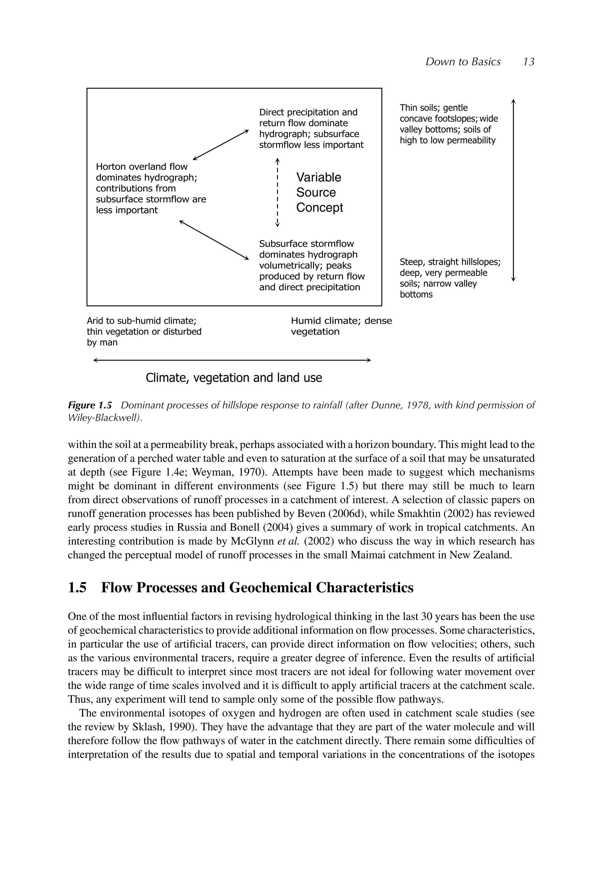
1.5 Dominant processes of hillslope response to rainfall (after Dunne, 1978, with kind
permission of Wiley-Blackwell). 13
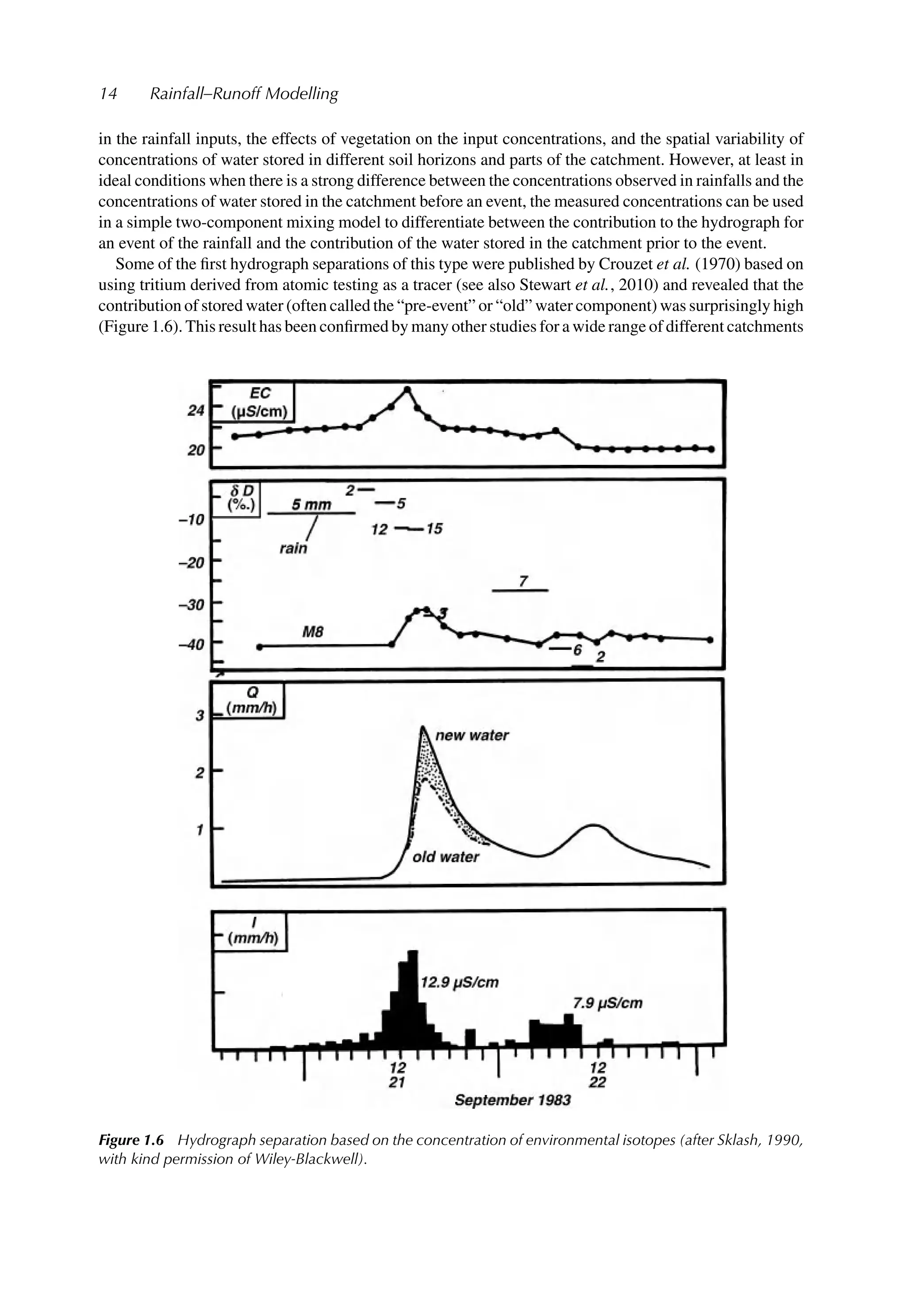
1.6 Hydrograph separation based on the concentration of environmental isotopes (after
Sklash, 1990, with kind permission of Wiley-Blackwell). 14
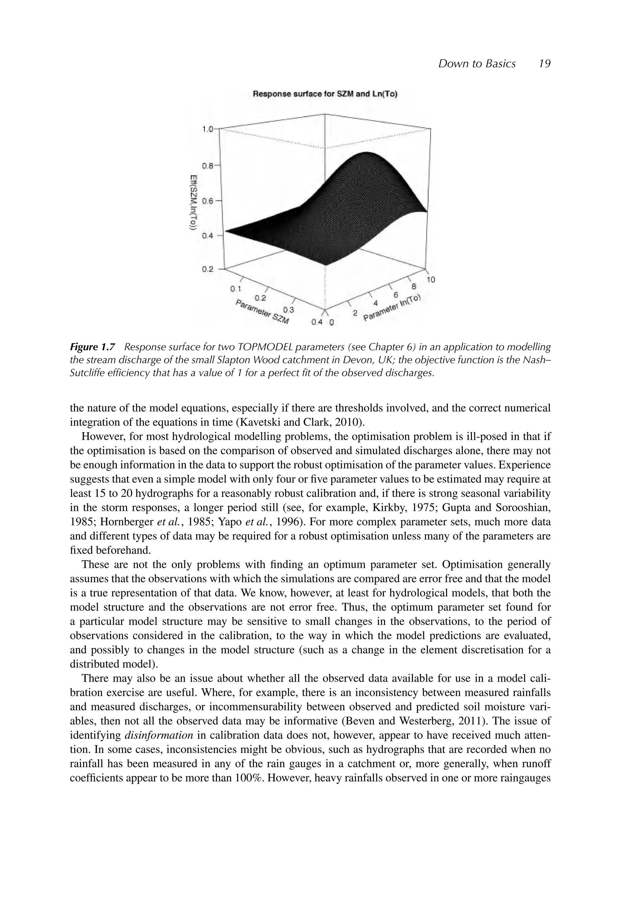
1.7 Response surface for two TOPMODEL parameters (see Chapter 6) in an
application to modelling the stream discharge of the small Slapton Wood
catchment in Devon, UK; the objective function is the Nash–Sutcliffe efficiency
that has a value of 1 for a perfect fit of the observed discharges. 19
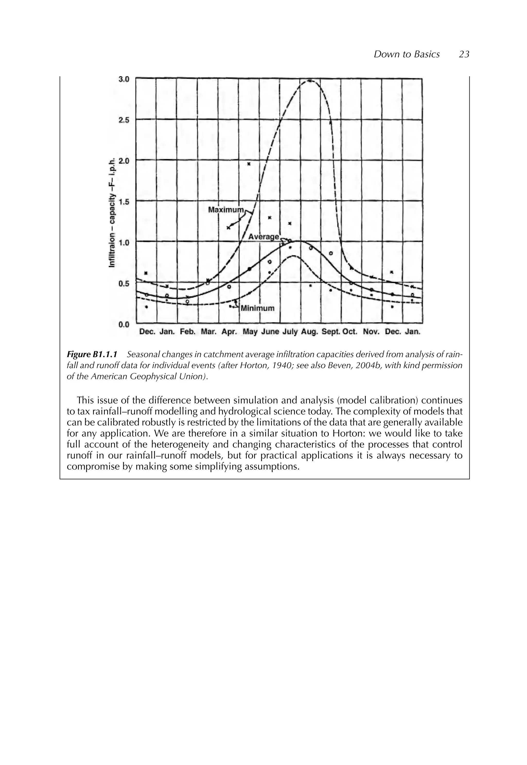
B1.1.1 Seasonal changes in catchment average infiltration capacities derived from analysis
of rainfall and runoff data for individual events (after Horton, 1940; see also Beven,
2004b, with kind permission of the American Geophysical Union). 23
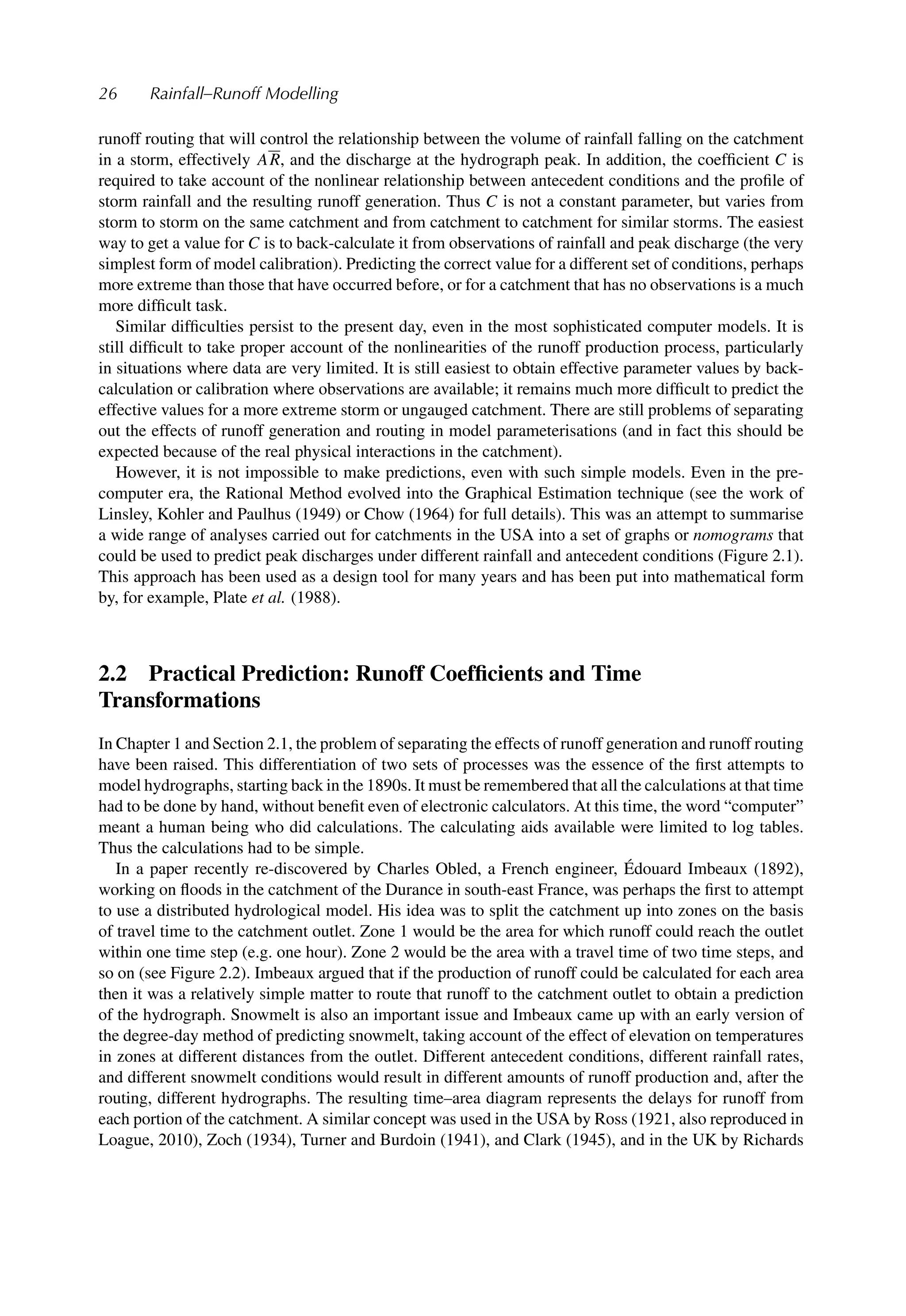
2.1 Graphical technique for the estimation of incremental storm runoff given an index
of antecedent precipitation, the week of the year, a soil water retention index and
precipitation in the previous six hours; arrows represent the sequence of use of the
graphs (after Linsley, Kohler and Paulhus, 1949). 27
2.2 Creating a time–area histogram by dividing a catchment into zones at different
travel times from the outlet (from Imbeaux, 1892). 28
2.3 Decline of infiltration capacity with time since start of rainfall: (a) rainfall intensity
higher than initial infiltration capacity of the soil; (b) rainfall intensity lower than
initial infiltration capacity of the soil so that infiltration rate is equal to the rainfall
rate until time to ponding, tp; fc is final infiltration capacity of the soil. 29
2.4 Methods of calculating an effective rainfall (shaded area in each case): (a) when
rainfall intensity is higher than the infiltration capacity of the soil, taking account
of the time to ponding if necessary; (b) when rainfall intensity is higher than some
constant “loss rate” (the φ index method); (c) when effective rainfall is a constant
proportion of the rainfall intensity at each time step. 31

xx List of Figures
2.5 Hydrograph separation into “storm runoff” and “baseflow” components: (a)
straight line separation (after Hewlett, 1974); (b) separation by recession curve
extension (after Reed et al., 1975). 32
2.6 The unit hydrograph as (a) a histogram; (b) a triangle; (c) a Nash cascade of N
linear stores in series. 34
2.7 A map of hydrological response units in the Little Washita catchment, Oklahoma,
USA, formed by overlaying maps of soils and vegetation classifications within a
raster geographical information system with pixels of 30 m. 36
2.8 Schematic diagram of the Dawdy and O’Donnell (1995) conceptual or explicit soil
moisture accounting (ESMA) rainfall–runoff model. 38
2.9 Observed and predicted discharges for the Kings Creek, Kansas (11.7 km2
) using
the VIC-2L model (see Box 2.2); note the difficulty of simulating the wetting up
period after the dry summer (after Liang et al. 1996, with kind permission
of Elsevier). 39
2.10 Results from the prediction of soil moisture deficit by Calder et al. (1983) for sites
in the UK: (a) the River Cam and (b) Thetford Forest; observed soil moisture
deficits are obtained by integrating over profiles of soil moisture measured by
neutron probe; input potential evapotranspiration was a simple daily climatological
mean time series (with kind permission of Elsevier). 39
B2.1.1 Nonlinearity of catchment responses revealed as a changing unit hydrograph for
storms with different volumes of rainfall inputs (after Minshall, 1960). 45
B2.2.1 Schematic diagram of the VIC-2L model (after Liang et al., 1994) with kind
permission of the American Geophysical Union. 48
B2.3.1 A control volume with local storage S, inflows Qi, local source or sink q, output
Qo and length scale x in the direction of flow. 50
3.1 Variations in rainfall in space and time for the storm of 27 June 1995 over the
Rapidan catchment, Virginia (after Smith et al., 1996, with kind permission of the
American Geophysical Union). 52
3.2 Measurements of actual evapotranspiration by profile tower, eddy correlation and
Bowen ratio techniques for a ranchland site in Central Amazonia (after Wright
et al., 1992, with kind permission of John Wiley and Sons). 59
3.3 Digital representations of topography: (a) vector representation of contour lines;
(b) raster grid of point elevations; (c) triangular irregular network representation. 62
3.4 Analysis of flow lines from raster digital elevation data: (a) single steepest descent
flow direction; (b) multiple direction algorithm of Quinn et al. (1995); (c) resultant
vector method of Tarboton (1997). 64
3.5 Analysis of flow streamlines from vector digital elevation data: (a) local analysis
orthogonal to vector contour lines; (b) TAPES-C subdivision of streamlines in the
Lucky Hills LH-104 catchment, Walnut Gulch, Arizona (after Grayson et al.
(1992a), with kind permission of the American Geophysical Union); (c) TIN
definition of flow lines in the Lucky Hills LH-106 catchment (after Palacios-Velez
et al., 1998, with kind permission of Elsevier). 65
3.6 Predicted spatial pattern of actual evapotranspiration based on remote sensing of
surface temperatures; note that these are best estimates of the evapotranspiration
rate at the time of the image; the estimates are associated with significant
uncertainty (after Franks and Beven, 1997b, with kind permission of the American
Geophysical Union). 69
3.7 Estimates of uncertainty in the extent of inundation of the 100-year return period
flood for the town of Carlisle, Cumbria, UK, superimposed on a satellite image of

List of Figures xxi
the area using GoogleMaps facilities; the inset shows the exceedance probabilities
for depth of inundation at the marked point (after Leedal et al., 2010). 71
B3.1.1 Schematic diagram of the components of the surface energy balance. Rn is net
radiation, λE is latent heat flux, C is sensible heat flux, A is heat flux due to
advection, G is heat flux to ground storage, S is heat flux to storage in the
vegetation canopy. The dotted line indicates the effective height of a “big leaf”
representation of the surface. 72
B3.1.2 Sensitivity of actual evapotranspiration rates estimated using the Penman–Monteith
equation for different values of aerodynamic and canopy resistance coefficients
(after Beven, 1979a, with kind permission of Elsevier). 75
B3.2.1 Schematic diagram of the Rutter interception model (after Rutter et al., 1971, with
kind permission of Elsevier). 77
B3.3.1 Discharge predictions for the Rio Grande basin at Del Norte, Colorado (3419 km2
)
using the Snowmelt Runoff model (SRM) based on the degree-day method (after
Rango, 1995, with kind permission of Water Resource Publications). 79
B3.3.2 Variation in average degree-day factor, F, over the melt season used in discharge
predictions in three large basins: the Dischma in Switzerland (43.3 km2
, 1668–
3146 m elevation range); the Dinwoody in Wyoming, USA (228 km2
, 1981–4202 m
elevation range); and the Durance in France (2170 km2
, 786–4105 m elevation
range) (after Rango, 1995, with kind permission of Water Resource Publications). 81
B3.3.3 Depletion curves of snow-covered area for different mean snowpack water
equivalent in a single elevation zone (2926–3353 m elevation range, 1284 km2
) of
the Rio Grande basin (after Rango, 1995, with kind permission of Water Resource
Publications). 82
4.1 Plots of the function g(Q) for the Severn and Wye catchments at Plynlimon: (a)
and (b) time step values of dQ
dt
against Q; (c) and (d) functions fitted to mean values
for increments of Q (after Kirchner, 2009, with kind permission of the American
4.2 Predicted hydrographs for the Severn and Wye catchments at Plynlimon (after
Kirchner, 2009, with kind permission of the American Geophysical Union). 86
4.3 A comparison of inferred and measured rainfalls at Plynlimon (after Kirchner,
2009, with kind permission of the American Geophysical Union). 87
4.4 A parallel transfer function structure and separation of a predicted hydrograph into
fast and slow responses. 88
4.5 Observed and predicted discharges using the IHACRES model for (a) Coweeta
Watershed 36 and (b) Coweeta Watershed 34: Top panel: observed and predicted
flows; middle panel: model residual series; lower panel: predicted total flow and
model identified slow flow component (after Jakeman and Hornberger, 1993, with
kind permission of the American Geophysical Union). 90
4.6 (a) Time variable estimates of the gain coefficient in the bilinear model for the CI6
catchment plotted against the discharge at the same time step; (b) optimisation of
the power law coefficient in fitting the observed discharges (after Young and
Beven, 1994, with kind permission of Elsevier). 94
4.7 Final block diagram of the CI6 bilinear power law model used in the predictions of
Figure 4.6 (after Young and Beven, 1994, with kind permission of Elsevier). 95
4.8 Observed and predicted discharges for the CI6 catchment at Llyn Briane, Wales,
using the bilinear power law model with n = 0.628 (after Young and Beven, 1994,
with kind permission of Elsevier). 95

xxii List of Figures
4.9 (a) Network and (b) network width function for River Hodder catchment (261km2
),
UK (after Beven and Wood, 1993, with kind permission of Wiley-Blackwell). 96
4.10 Strahler ordering of a river network as used in the derivation of the
geomorphological unit hydrograph. 98
4.11 The structure of a neural network showing input nodes, output nodes and a single
layer of hidden nodes; each link is associated with at least one coefficient (which
may be zero). 100
4.12 Application of a neural network to forecasting flows in the River Arno catchment,
northern Italy: one- and six-hour-ahead forecasts are based on input data of lagged
rainfalls, past discharges, and power production information; the influence of
power production on the flow is evident in the recession periods (after Campolo
et al., 2003, with kind permission of Taylor and Francis). 101
4.13 Application of an SVM method to predict flood water levels in real time, with lead
times of one to six hours (after Yu et al., 2006, with kind permission of Elsevier). 102
4.14 WS2 catchment, H J Andrews Forest, Oregon: (a) depth 5 regression tree and (b)
discharge prediction using a regression tree with 64 terminal nodes (after
Iorgulescu and Beven, 2004, with kind permission of the American Geophysical
Union). 104
B4.1.1 The linear store. 107
B4.3.1 Nonparametric state dependent parameter estimation of the gain coefficient in the
identification of a data-based mechanistic (DBM) model using daily data at
Coweeta (after Young, 2000, with kind permission of Wiley-Blackwell). 115
B4.3.2 Predicted discharge from a DBM model for Coweeta using the input nonlinearity
of Figure B4.3.1 (after Young, 2000, with kind permission of Wiley-Blackwell).
Peter Young also shows in this paper how this model can be improved even further
by a stochastic model of a seasonal function of temperature, representing a small
effect of evapotranspiration on the dynamics of runoff production. 116
5.1 Finite element discretisation of a vertical slice through a hillslope using a mixed
grid of triangular and quadrilateral elements with a typical specification of
boundary conditions for the flow domain; the shaded area represents the saturated
zone which has risen to intersect the soil surface on the lower part of the slope. 122
5.2 Schematic diagram for surface flows with slope So and distance x measured along
the slope: (a) one-dimensional representation of open channel flow with discharge
Q, cross-sectional area A, wetted perimeter P, average velocity v and average
depth y; (b) one-dimensional representation of overland flow as a sheet flow with
specific discharge q, width W, average velocity v and average depth h. 125
5.3 Schematic diagram of a grid-based catchment discretisation as in the SHE model
(after Refsgaard and Storm, 1995, with kind permission from Water Resource
Publications). 129
5.4 Schematic diagram of a hillslope plane catchment discretisation as in the IHDM
model (after Calver and Wood, 1995, with kind permission from Water Resource
Publications). 130
5.5 Process-based modelling of the Reynolds Creek hillslope: (a) topography, geology
and instrumentation; (b) discretisation of the hillslope for the finite difference
model; (c) calibrated transient simulation results for 5 April to 13 July 1971 melt
season (after Stephenson and Freeze, 1974, with kind permission of the American
5.6 Results of the Bathurst and Cooley (1996) SHE modelling of the Upper Sheep
Creek subcatchment of Reynolds Creek: (a) Using the best-fit energy budget

List of Figures xxiii
snowmelt model; (b) using different coefficients in a degree-day snowmelt model
(with kind permission of Elsevier). 137
5.7 SHE model blind evaluation tests for Slapton Wood catchment, Devon, UK
(1/1/90–31/3/91): (a) comparison of the predicted phreatic surface level bounds for
square (14; 20) with the measured levels for dipwell (14; 18); (b) comparison of the
predicted bounds and measured weekly soil water potentials at square (10; 14) for
1.0 m depth (after Bathurst et al., 2004, with kind permission of Elsevier). 139
5.8 SHE model blind evaluation tests for Slapton Wood catchment, Devon, UK
(1/1/90–31/3/91): (a) comparison of the predicted discharge bounds and measured
discharge for the Slapton Wood outlet weir gauging station; (b) comparison of the
predicted discharge bounds and measured monthly runoff totals for the outlet weir
gauging station (after Bathurst et al., 2004, with kind permission of Elsevier). 140
5.9 A comparison of different routing methods applied to a reach of the River Yarra,
Australia (after Zoppou and O’Neill, 1982). 142
5.10 Wave speed–discharge relation on the Murrumbidgee River over a reach of 195 km
between Wagga Wagga and Narrandera (after Wong and Laurenson, 1983, with
kind permission of the American Geophysical Union): Qb1 is the reach flood
warning discharge; Qb2 is the reach bankfull discharge. 143
5.11 Average velocity versus discharge measurements for several reaches in the Severn
catchment at Plynlimon, Wales, together with a fitted function of the form of
Equation (5.10) that suggests a constant wave speed of 1 ms−1
(after Beven, 1979,
with kind permission of the American Geophysical Union). 144
5.12 Results of modelling runoff at the plot scale in the Walnut Gulch catchment: (a) the
shrubland plot and (b) the grassland plot; the error bars on the predictions indicate
the range of 10 randomly chosen sets of infiltration parameter values (after Parsons
5.13 Results of modelling the 4.4 ha Lucky Hills LH-104 catchment using KINEROS
with different numbers of raingauges to determine catchment inputs (after Faurès
et al., 1995, with kind permission of Elsevier). 150
5.14 Patterns of infiltration capacity on the R-5 catchment at Chickasha, OK: (a)
distribution of 247 point measurements of infiltration rates; (b) distribution of
derived values of intrinsic permeability with correction to standard temperature;
(c) pattern of saturated hydraulic conductivity derived using a kriging interpolator;
(d) pattern of permeability derived using kriging interpolator (after Loague and
Kyriakidis, 1997, with kind permission of the American Geophysical Union). 152
B5.2.1 Predictions of infiltration equations under conditions of surface ponding. 160
B5.2.2 Variation of Green–Ampt infiltration equation parameters with soil texture (after
Rawls et al., 1983, with kind permission from Springer Science+Business
Media B.V). 163
B5.3.1 Discretisations of a hillslope for approximate solutions of the subsurface flow
equations: (a) Finite element discretisation (as in the IHDM); (b) Rectangular finite
difference discretisation (as used by Freeze, 1972); (c) Square grid in plan for
saturated zone, with one-dimensional vertical finite difference discretisation for the
unsaturated zone (as used in the original SHE model). 167
B5.3.2 Schematic diagram of (a) explicit and (b) implicit time stepping strategies in
approximate numerical solutions of a partial differential equation, here in one
spatial dimension, x (arrows indicate the nodal values contributing to the solution
for node (i, t + 1); nodal values in black are known at time t; nodal values in grey
indicate dependencies in the solution for time t + 1). 168

xxiv List of Figures
B5.4.1 Comparison of the Brooks–Corey and van Genuchten soil moisture characteristics
functions for different values of capillary potential: (a) soil moisture content and
(b) hydraulic conductivity. 172
B5.4.2 Scaling of two similar media with different length scales α. 173
B5.4.3 Scaling of unsaturated hydraulic conductivity curves derived from field infiltration
measurements at 70 sites under corn rows on Nicollet soil, near Boone, Iowa (after
Shouse and Mohanty, 1998, with kind permission of the American Geophysical Union). 175
B5.5.1 A comparison of values of soil moisture at capillary potentials of -10 and -100 cm
curves fitted to measured data and estimated using the pedotransfer functions of
Vereeken et al. (1989) for different locations on a transect (after Romano and
Santini, 1997, with kind permission of Elsevier). 177
B5.6.1 Ranges of validity of approximations to the full St. Venant equations defined in
terms of the dimensionless Froude and kinematic wave numbers (after Daluz
Vieira, 1983, with kind permission of Elsevier). 180
6.1 Structure of the Probability Distributed Moisture (PDM) model. 187
6.2 Integration of PDM grid elements into the G2G model (after Moore et al., 2006,
with kind permission of IAHS Press). 189
6.3 Definition of the upslope area draining through a point within a catchment. 190
6.4 The ln(a/ tan β) topographic index in the small Maimai M8 catchment (3.8 ha),
New Zealand, calculated using a multiple flow direction downslope flow algorithm;
high values of topographic index in the valley bottoms and hillslope hollows
indicate that these areas are predicted as saturating first (after Freer, 1998). 192
6.5 Distribution function and cumulative distribution function of topographic index
values in the Maimai M8 catchment (3.8 ha), New Zealand, as derived from the
pattern of Figure 6.4. 193
6.6 Spatial distribution of saturated areas in the Brugga catchment (40 km2
), Germany:
(a) mapped saturated areas (6.2% of catchment area); (b) topographic index
predicted pattern at same fractional catchment area assuming a homogeneous soil
(after Güntner et al., 1999, with kind permission of John Wiley and Sons). 196
6.7 Application of TOPMODEL to the Saeternbekken MINIFELT catchment, Norway
(0.75 ha): (a) topography and network of instrumentation; (b) pattern of the
ln(a/ tan β) topographic index; (c) prediction of stream discharges using both
exponential (EXP) and generalised (COMP) transmissivity functions (after Lamb
6.8 Predicted time series of water table levels for the four recording boreholes in the
Saeternbekken MINIFELT catchment, Norway, using global parameters calibrated
on catchment discharge and recording borehole data from an earlier snow-free
period in October–November 1987 (after Lamb et al., 1997, with kind permission
of John Wiley and Sons). 201
6.9 Predicted local water table levels for five discharges (0.1 to 6.8 mm/hr) in the
Saeternbekken MINIFELT catchment, Norway, using global parameters calibrated
on catchment discharge and recording borehole data from October–November
1987 (after Lamb et al., 1997, with kind permission of John Wiley and Sons). 202
6.10 Relationship between storm rainfall and runoff coefficient as percentage runoff
predicted by the USDA-SCS method for different curve numbers. 206
B6.1.1 Schematic diagram of prediction of saturated area using increments of the
topographic index distribution in TOPMODEL. 212
B6.1.2 Derivation of an estimate for the TOPMODEL m parameter using recession curve
analysis under the assumption of an exponential transmissivity profile and
negligible recharge. 215

List of Figures xxv
B6.1.3 Use of the function G(Ac
) to determine the critical value of the topographic index at
the edge of the contributing area given D
m
, assuming a homogeneous transmissivity
(after Saulnier and Datin, 2004, with kind permission of John Wiley and Sons). 218
B6.2.1 Definition of hydrological response units for the application of the SWAT model to
the Colworth catchment in England as grouped grid entities of similar properties
(after Kannan et al., 2007, with kind permission of Elsevier). 222
B6.2.2 Predictions of streamflow for the Colworth catchment using the revised ArcView
SWAT2000 model: validation period (after Kannan et al., 2007, with kind
permission of Elsevier). 223
B6.3.1 Variation in effective contributing area with effective rainfall for different values of
Smax (after Steenhuis et al., 1995, with kind permission of the American Society of
Civil Engineers); effective rainfall is here defined as the volume of rainfall after the
start of runoff, P − Ia. 227
B6.3.2 Application of the SCS method to data from the Mahatango Creek catchment
(55 ha), Pennsylvania (after Steenhuis et al., 1995, with kind permission of the
American Society of Civil Engineers); effective rainfall is here defined as the
volume of rainfall after the start of runoff. 228
7.1 Response surface for two parameter dimensions with goodness of fit represented as
contours. 234
7.2 More complex response surfaces in two parameter dimensions: (a) flat areas of the
response surface reveal insensitivity of fit to variations in parameter values; (b)
ridges in the response surface reveal parameter interactions; (c) multiple peaks in
the response surface indicate multiple local optima. 235
7.3 Generalised (Hornberger–Spear–Young) sensitivity analysis – cumulative
distributions of parameter values for: (a) uniform sampling of prior parameter
values across a specified range; (b) behavioural and nonbehavioural simulations for
a sensitive parameter; (c) behavioural and nonbehavioural simulations for an
insensitive parameter. 238
7.4 Comparing observed and simulated hydrographs. 240
7.5 (a) Empirical distribution of rainfall multipliers determined using BATEA in an
application of the GR4 conceptual rainfall–runoff model to the Horton catchment
in New South Wales, Australia; the solid line is the theoretical distribution
determined from the identification process; note the log transformation of the
multipliers: the range −1 to 1 represents values of 0.37 to 2.72 applied to
individual rainstorms in the calibration period; the difference from the theoretical
distribution is attributed to a lack of sensitivity in identifying the multipliers in the
mid-range, but may also indicate that the log normal distribution might not be a
good assumption in this case; (b) validation period hydrograph showing model and
total uncertainty estimates (reproduced from Thyer et al. (2009) with kind
permission of the American Geophysical Union). 248
7.6 Iterative definition of the Pareto optimal set using a population of parameter sets
initially chosen randomly: (a) in a two-dimensional parameter space (parameters
X1, X2); (b) in a two-dimensional performance measure space (functions F1, F2);
(c) and (d) grouping of parameter sets after one iteration; (e) and (f) grouping of
parameter sets after four iterations; after the final iteration, no model with
parameter values outside the Pareto optimal set has higher values of the
performance measures than the models in the Pareto set (after Yapo et al., 1998,

xxvi List of Figures
7.7 Pareto optimal set calibration of the Sacramento ESMA rainfall–runoff model to
the Leaf River catchment, Mississippi (after Yapo et al., 1998, with kind
permission of Elsevier): (a) grouping of Pareto optimal set of 500 model parameter
sets in the plane of two of the model parameters; (b) prediction limits for the 500
Pareto optimal parameter sets. 251
7.8 An application of TOPMODEL to the Maimai M8 catchment (3.8 ha), New
Zealand, using the GLUE methodology: (a) dotty plots of the Nash–Sutcliffe
model efficiency measure (each dot represents one run of the model with parameter
values chosen randomly by uniform sampling across the ranges of each parameter);
(b) discharge prediction limits for a period in 1987, after conditioning using
observations from 1985 and 1986. 253
7.9 Rescaled likelihood weighted distributions for TOPMODEL parameters,
conditioned on discharge and borehole observations from the Saeternbekken
MINIFELT catchment for the autumn 1987 period (after Lamb et al., 1998b, with
kind permission of Elsevier). 259
7.10 Prediction bounds for stream discharge from the Saeternbekken catchment for the
1989 simulations, showing prior bounds after conditioning on the 1987 simulation
period and posterior bounds after additional updating with the 1989 period data
(after Lamb et al., 1998b, with kind permission of Elsevier). 260
7.11 Prediction bounds for four recording boreholes in the Saeternbekken catchment for
the 1989 simulation period, showing prior bounds after conditioning on the 1987
simulation period and posterior bounds after additional updating with the 1989
period data (after Lamb et al., 1998b, with kind permission of Elsevier). 261
7.12 Prediction bounds for spatially distributed piezometers in the Saeternbekken
catchment for three different discharges, showing prior bounds after conditioning
on discharge and recording borehole observations, bounds based on conditioning
on the piezometer data alone and posterior bounds based on a combination of both
individual measures (after Lamb et al., 1998b, with kind permission of Elsevier). 262
7.13 Uncertainty in the rating curve for the River Brue catchment with assumed limits of
acceptability bounds for model simulations (calculations by Philip Younger)
(Calculations by Philip Younger). 263
7.14 Model residuals as time series of scaled scores for two runs of dynamic
TOPMODEL as applied to the River Brue catchment, Somerset, England. The
horizontal lines at −1, 0, and +1 represent the lower limit of acceptability, observed
value and upper limit of acceptability respectively (calculations by Philip Younger). 263
7.15 A comparison of reconstructed model flow and observed flow for the validation
period, 18–28 November 1996: the reconstructed flow is shown by the middle
dotted line and was created by taking the median value of the reconstructed flows
from all of the behavioural models at each time step; the outer dotted lines show the
5th and 95th percentiles of the reconstructed model flow; the dashed lines show the
5th and 95th percentiles of the unreconstructed behavioural models; the continuous
line is the observed flow; the shaded grey area shows the limits of acceptability
applied to the observed discharges for this period (calculations by Philip Younger). 264
7.16 Observed and predicted daily discharges simulated by a version of TOPMODEL
for the small Ringelbach catchment (34 ha), Vosges, France: the model was run
using an 18-minute time step; note the logarithmic discharge scale; prediction
limits are estimated using the GLUE methodology (after Freer et al. 1996, with
kind permission of the American Geophysical Union). 266

List of Figures xxvii
7.17 Observed and WASMOD simulated discharge (top) for 1984 in the Paso La Ceiba
catchment, Honduras; at the end of October, a period of disinformative data can be
seen; the second, third and fourth plots from the top show the effect of the
disinformative data on the residual sum of squares, the Nash–Sutcliffe efficiency
and the magnitude of the residuals (from Beven and Westerberg, 2011, with kind
permission of John Wiley and Sons). 270
7.18 The South Tyne at Featherstone: (a) Master recession curve and (b) example of
event separation (after Beven et al., 2011). 272
7.19 The South Tyne at Featherstone: estimated runoff coefficients for events; black
circles have values between 0.3 and 0.9 (after Beven et al., 2011). 273
B7.1.1 A normal quantile transform plot of the distribution of the actual model residuals
(horizontal axis) against the standardised scores for the normal or Gaussian
distribution (vertical axis) (after Montanari and Brath, 2004, with kind permission
of the American Geophysical Union). 278
B7.1.2 Residual scores. 281
B7.1.3 Conversion of scores to likelihoods. 282
8.1 Cascade of flood forecasting system components in the River Eden, Cumbria, UK:
The model assimilates data at each gauging station site (circles) and generates
forecasts for Sheepmount with a six-hour lead time (after Leedal et al., 2008, with
kind permission of the CRC Press/Balkema). 297
8.2 Identified input nonlinearities for each of the forecasting system components in the
River Eden, Cumbria, UK: (a) input nonlinearities for Model 1 in Figure 8.1;
(b) input nonlinearities for Model 2 in Figure 8.1; (c) input nonlinearities for
Model 3 in Figure 8.1 (after Leedal et al., 2008, with kind permission of the CRC
Press/Balkema). 298
8.3 Adaptive six-hour ahead forecasts for Sheepmount gauging station, Carlisle, with
5% and 95% uncertainty estimates for the January 2005 flood event (after Leedal
et al., 2008, with kind permission of the CRC Press/Balkema). 299
8.4 Subcatchments and observation sites in the Skalka catchment in the Czech
Republic (672 km2
) (after Blazkova and Beven, 2009, with kind permission of the
8.5 Flood frequency curve at the Cheb gauging station: circles are the observed annual
flood peaks (1887–1959); grey lines are the 4192 simulations, each of 10 000 years
of hourly data, with scores on all criteria 1.48; dashed lines are the 5% and 95%
possibility bounds from the trapezoidal weighting; thin black lines are the
behavioral simulations with scores on all criteria 1 for the initial 67-year
simulations (after Blazkova and Beven, 2009, with kind permission of the
B8.1.1 Comparison of adaptive and non-adaptive five-hour-ahead flood forecasts on the
River Nith (after Lees et al., 1994, with kind permission of John Wiley and Sons). 312
9.1 Three-dimensional view of an ensemble of three REWs, including a portion of
atmosphere (after Reggiani and Rientjes, 2005, with kind permission of the
9.2 Normalised storage (r(t) = V(t)/Vmax)) versus flux (u(t) = Q(L, t)/Qmax)
relationships for four hillslope forms: 1. divergent concave; 3. divergent convex;
7. convergent concave; and 9. convergent convex (after Norbiato and Borga, 2008,
9.3 (a) Saturated area ratio (SAR) against relative water content (RWC) for a five-year
simulation period of the Reno catchment at the Calcara river section (grey dots);
the steady state curve (SS) was obtained as a set of SAR–RWC values for different

xxviii List of Figures
simulations relative to precipitation events of different intensity and after the
equilibrium state has been reached; the drying curve (DC) represents the SAR and
RWC values for the drying down transition phase only; (b) Schematic diagram
showing how the hysteretic relationship is used in the lumped TOPKAPI model
(after Martina et al., 2011, with kind permission of Elsevier). 321
9.4 Distribution of unsaturated zone (light grey), saturated zone (darker grey) and
tracer (black) particles in the MIPs simulation of a tracer experiment at Gårdsjön,
Sweden (after Davies et al., 2011, with kind permission of John Wiley
and Sons). 322
9.5 (a) a series of rainfall events on slopes of 40, 80 and 160 m length: (b) hydrograph
and (c) storage flux relationships under dry antecedent conditions; (d) hydrograph
and (e) storage flux relationships under wet initial conditions; both sets of results
were produced using the MIPs random particle tracking simulator on slopes of 2.86
degrees, with a constant soil depth of 1.5 m and a constant hydraulic conductivity at
the soil surface of 50 m/day, declining exponentially with depth (calculations by
Jessica Davies). 323
10.1 Hydrograph predictions using the PDM model and parameters estimated by the
ensemble method: (a) the 10 best parameter sets from the 10 most similar
catchments; (b) 90th percentile of the same ensemble; (c) similarity weighted
ensemble (after McIntyre et al., 2005, with kind permission of the American
10.2 Simulation results for the Harrowdown Old Mill catchment (194 km2
) treated as if
ungauged with observed and ensemble prediction streamflows (the grey range is
the unconstrained ensemble; the white range is the ensemble constrained by
predicted hydrograph indices) (after Zhang et al., 2008, with kind permission of
the American Geophysical Union). 338
10.3 (a) Model efficiencies for the entire 10-year period of the weighted ensemble mean
where the ensemble has been selected based on n randomly chosen measurements
during one year: the solid line and the circles represent the median over all years,
catchments and random realisations of the selection of n days; the dashed lines
show the medians of the percentiles (10% and 90%) for the different realisations of
the selection of n days; (b) performance of different strategies to select six days of
observations during one year for use in model calibration; black dots represent the
median of 10 years for one catchment; squares represent the median of all
catchments (after Seibert and Beven, 2009). 341
11.1 Predicted contributions to individual hydrographs from different precipitation
inputs (grey shading); this hypothetical simulation uses the MIPs model of Davies
et al. (2011) on a 160 m hillslope with a soil depth of 1.5 m and a hydraulic
conductivity profile similar to that found at the Gårdsjön catchment, Sweden (see
Figure 11.8). 345
11.2 Mixing diagram for direct precipitation, soil water and groundwater end members
defined for silica and calcium in the Haute-Mentue catchment, Switzerland (after
Iorgulescu et al., 2005, with kind permission of John Wiley and Sons). 348
11.3 Observed and predicted discharges, silica and calcium concentrations for the
Bois-Vuacoz subcatchment; lines represent the range and quantiles of the
predictions from the 216 behavioural models (after Iorgulescu et al., 2005, with
kind permission of John Wiley and Sons). 350
11.4 Changing contributions of the different components of stream flow in the
Bois-Vuacoz subcatchment as a function of storage; results are the median

List of Figures xxix
estimates over 216 behavioural models (after Iorgulescu et al., 2005, with kind
permission of John Wiley and Sons). 351
11.5 Prediction of stream 18
O isotope concentrations for the Bois-Vuacoz subcatchment
(from Iorgulescu et al., 2007, with kind permission of the American
11.6 Inferred dynamic storages for (a) soil water and (b) direct precipitation from
modelling isotope concentrations in the Bois-Vuacoz subcatchment (from
Iorgulescu et al., 2007, with kind permission of the American Geophysical Union). 352
11.7 A comparison of mean travel times estimated from observations (MTTGM) and
those estimated from catchment characteristics (MTTCC) for catchments in
Scotland (from Soulsby et al., 2010, with kind permission of John Wiley and
Sons). Error bars represent 5 and 95% percentiles. 355
11.8 A representation of particle velocities chosen from an exponential distribution for
each layer in a way consistent with the nonlinear profile of hydraulic conductivity
at Gårdsjön (after Davies et al., 2011, with kind permission of John Wiley and Sons). 358
11.9 Observed and predicted flow and tracer concentrations for the Trace B experiment
at Gårdsjön, Sweden; the first three hypotheses about the tracer movement were
rejected as inconsistent with the observations; the hydrograph simulation was based
only on field data and the assumed velocity distribution of Figure (11.8) without
calibration (after Davies et al., 2011, with kind permission of John Wiley and Sons). 359
B11.1.1 Solution of the advection–dispersion equation (Equation (B11.1.4)): (a) plotted
against distance in the flow direction; (b) plotted against time for a single point in space. 362
B11.1.2 Fit of the aggregated dead zone model to a tracer experiment for the Colorado
River for the Hance Rapids to Diamond reach (238.8 km). 364
B11.2.1 Forms of the gamma distribution for different values of the parameters K and N. 366

1
Down to Basics: Runoff Processes
and the Modelling Process
As scientists we are intrigued by the possibility of assembling our knowledge into a neat
package to show that we do, after all, understand our science and its complex interrelated
phenomena.
W. M. Kohler, 1969
Remember that the computer is a tool for simulation, and what is simulated becomes the
reality of the user. In a society like ours – the post-modern society – there are no ‘great
stories’ to justify a specific perception of reality like there were in the 19th century. We
should rather see the situation thus: communication is based on a number of language
games which are played according to specific sets of rules. Each group of society can ‘play
a game’, and thus it is the efficiency of each game that justifies it. The computer medium
should be seen as a technical device that allows its owner to play particularly efficient
games. . . . A good program is one that creates the reality intended by the sender in the most
efficient way.
P. B. Andersen and L. Mathiessen, 1987
1.1 Why Model?
As noted in the preface, there are many reasons why we need to model the rainfall–runoff processes of
hydrology. The main reason is a result of the limitations of hydrological measurement techniques. We
are not able to measure everything we would like to know about hydrological systems. We have, in fact,
only a limited range of measurement techniques and a limited range of measurements in space and time.
We therefore need a means of extrapolating from those available measurements in both space and time,
particularly to ungauged catchments (where measurements are not available) and into the future (where
measurements are not possible) to assess the likely impact of future hydrological change. Models of
Rainfall–Runoff Modelling: The Primer, Second Edition. Keith Beven.
© 2012 John Wiley Sons, Ltd. Published 2012 by John Wiley Sons, Ltd.

2 Rainfall–Runoff Modelling
different types provide a means of quantitative extrapolation or prediction that will hopefully be helpful
in decision making.
There is much rainfall–runoff modelling that is carried out purely for research purposes as a means
of formalising knowledge about hydrological systems. The demonstration of such understanding is an
important way of developing an area of science. We generally learn most when a model or theory is shown
to be in conflict with reliable data so that some modification of the understanding on which the model is
based must be sought. However, the ultimate aim of prediction using models must be to improve decision
making about a hydrological problem, whether that be in water resources planning, flood protection,
mitigation of contamination, licensing of abstractions, or other areas. With increasing demands on water
resourcesthroughouttheworld,improveddecisionmakingwithinacontextoffluctuatingweatherpatterns
from year to year requires improved models. That is what this book is about.
Rainfall–runoff modelling can be carried out within a purely analytical framework based on obser-
vations of the inputs to and outputs from a catchment area. The catchment is treated as a black box,
without any reference to the internal processes that control the transformation of rainfall to runoff. Some
models developed in this way are described in Chapter 4, where it is shown that it may also be pos-
sible to make some physical interpretation of the resulting models based on an understanding of the
nature of catchment response. This understanding should be the starting point for any rainfall–runoff
modelling study.
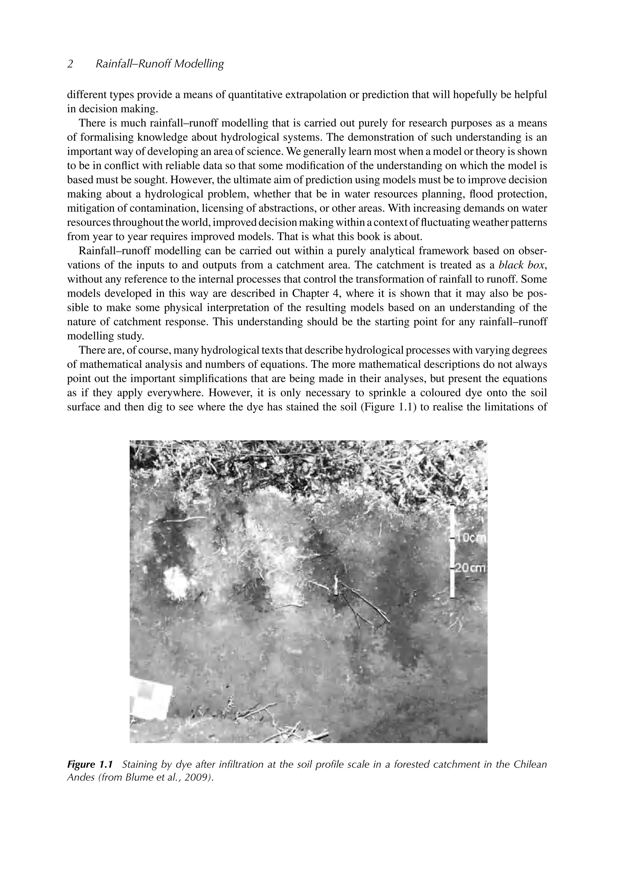
There are, of course, many hydrological texts that describe hydrological processes with varying degrees
of mathematical analysis and numbers of equations. The more mathematical descriptions do not always
point out the important simplifications that are being made in their analyses, but present the equations
as if they apply everywhere. However, it is only necessary to sprinkle a coloured dye onto the soil
surface and then dig to see where the dye has stained the soil (Figure 1.1) to realise the limitations of
Figure 1.1 Staining by dye after infiltration at the soil profile scale in a forested catchment in the Chilean
Andes (from Blume et al., 2009).

Down to Basics 3
hydrological theory (see also Flury et al., 1994; Zehe and Flühler, 2001; Weiler and Naef, 2003; Kim
et al., 2006; Blume et al., 2009). Whenever detailed studies of flow pathways are carried out in the field
we find great complexity. We can perceive that complexity quite easily, but producing a mathematical
description suitable for quantitative prediction is much more difficult and will always involve important
simplication and approximation. This initial chapter will, therefore, be concerned with a perceptual model
of catchment response as the first stage of the modelling process. This complexity is one reason why
there is no commonly agreed modelling strategy for the rainfall–runoff process but a variety of options
and approaches that will be discussed in the chapters that follow.
1.2 How to Use This Book
It should be made clear right at the beginning that this book is not only about the theory that underlies
the different types of rainfall–runoff model that are now available to the user. You will find, for example,
that relatively few equations are used in the main text of the book. Where it has been necessary to show
some theoretical development, this is generally presented in boxes at the ends of the chapters that can
be skipped at a first reading. The theory can also be followed up in the many (but necessarily selected)
references quoted, if necessary.
This is much more a book about the concepts that underlie different modelling approaches and the
critical analysis of the software packages that are now widely available for hydrological prediction. The
presentation of models as software is becoming increasingly sophisticated with links to geographical
information systems and the display of impressive three-dimensional graphical outputs. It is easy to be
seduced by these displays into thinking that the output of the model is a good simulation of the real
catchment response, especially if little data are available to check on the predictions. However, even the
most sophisticated models currently available are not necessarily good simulations and evaluation of the
model predictions will be necessary. It is hoped that the reader will learn from this book the concepts
and techniques necessary to evaluate the assumptions that underlie the different modelling approaches
and packages available and the issues of implementing a model for a particular application.
One of the aims of this book is to train the reader to evaluate models, not only in terms of how well the
model can reproduce any data that are available for testing, but also by critically assessing the assumptions
made. Thus, wherever possible, models are presented with a list of the assumptions made. The reader is
encouraged to make a similar list when encountering a model for the first time. At the end of each chapter,
a review of the major points arising from that chapter has been provided. It is generally a good strategy
to read the summary before reading the bulk of the chapter. Some sources of rainfall–runoff modelling
software are listed in Appendix A. A glossary of terms used in hydrological modelling is provided in
Appendix B. These terms are highlighted when they first appear in the text.
This edition has been extended, relative to the first edition, particularly in respect of the chapters
labelled “Beyond the Primer”. New material on the next generation of hydrological models, modelling
ungauged catchments, and modelling sources and residence time distributions of water have been added.
In addition, there has been a lot of research in the last decade on the use of distributed models and
the treatment of uncertainty in hydrological predictions so that Chapters 5, 6 and 7 have also been
substantially revised.
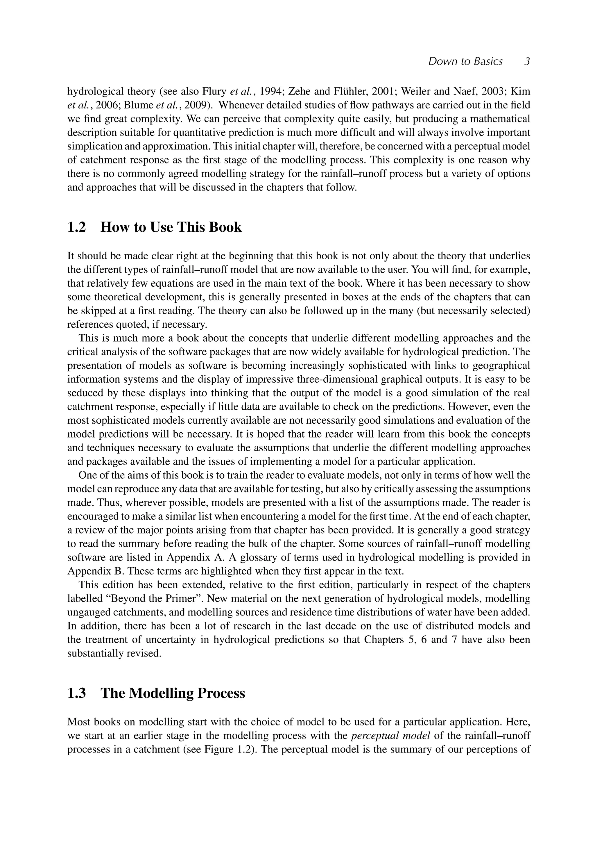
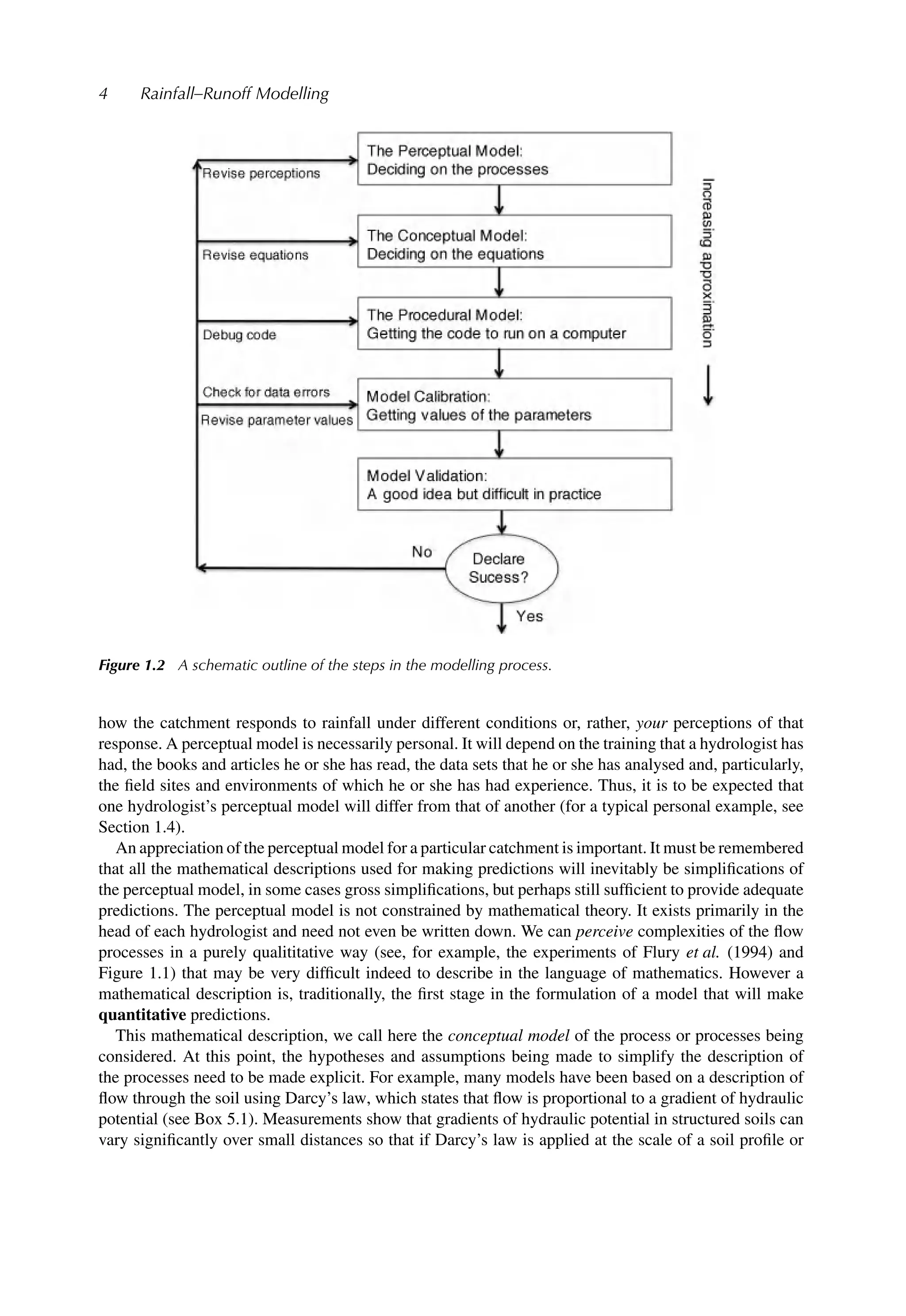
1.3 The Modelling Process
Most books on modelling start with the choice of model to be used for a particular application. Here,
we start at an earlier stage in the modelling process with the perceptual model of the rainfall–runoff
processes in a catchment (see Figure 1.2). The perceptual model is the summary of our perceptions of

Figure 1.2 A schematic outline of the steps in the modelling process.
how the catchment responds to rainfall under different conditions or, rather, your perceptions of that
response. A perceptual model is necessarily personal. It will depend on the training that a hydrologist has
had, the books and articles he or she has read, the data sets that he or she has analysed and, particularly,
the field sites and environments of which he or she has had experience. Thus, it is to be expected that
one hydrologist’s perceptual model will differ from that of another (for a typical personal example, see
Section 1.4).
An appreciation of the perceptual model for a particular catchment is important. It must be remembered
that all the mathematical descriptions used for making predictions will inevitably be simplifications of
the perceptual model, in some cases gross simplifications, but perhaps still sufficient to provide adequate
predictions. The perceptual model is not constrained by mathematical theory. It exists primarily in the
head of each hydrologist and need not even be written down. We can perceive complexities of the flow
processes in a purely qualititative way (see, for example, the experiments of Flury et al. (1994) and
Figure 1.1) that may be very difficult indeed to describe in the language of mathematics. However a
mathematical description is, traditionally, the first stage in the formulation of a model that will make
quantitative predictions.
This mathematical description, we call here the conceptual model of the process or processes being
considered. At this point, the hypotheses and assumptions being made to simplify the description of
the processes need to be made explicit. For example, many models have been based on a description of
flow through the soil using Darcy’s law, which states that flow is proportional to a gradient of hydraulic
potential (see Box 5.1). Measurements show that gradients of hydraulic potential in structured soils can
vary significantly over small distances so that if Darcy’s law is applied at the scale of a soil profile or

Down to Basics 5
greater, it is implicitly assumed that some average gradient can be used to characterise the flow and that
the effects of preferential flow through macropores in the soil (one explanation of the observations of
Figure 1.1) can be neglected. It is worth noting that, in many articles and model user manuals, while the
equations on which the model is based may be given, the underlying simplifying assumptions may not
actually be stated explicitly. Usually, however, it is not difficult to list the assumptions once we know
something of the background to the equations. This should be the starting point for the evaluation of a
particular model relative to the perceptual model in mind. Making a list of all the assumptions of a model
is a useful practice that we follow here in the presentation of different modelling approaches.
The conceptual model may be more or less complex, ranging from the use of simple mass balance
equations for components representing storage in the catchment to coupled nonlinear partial differential
equations. Some equations may be easily translated directly into programming code for use on a digital
computer. However, if the equations cannot be solved analytically given some boundary conditions for the
real system (which is usually the case for the partial differential equations found in hydrological models)
then an additional stage of approximation is necessary using the techniques of numerical analysis to define
a procedural model in the form of code that will run on the computer. An example is the replacement of
the differentials of the original equations by finite difference or finite volume equivalents. Great care has
to be taken at this point: the transformation from the equations of the conceptual model to the code of
the procedural model has the potential to add significant error relative to the true solution of the original
equations. This is a particular issue for the solution of nonlinear continuum differential equations but
has been the subject of recent discussion with respect to more conceptual catchment models (Clark and
Kavetski, 2010). Because such models are often highly nonlinear, assessing the error due only to the
implementation of a numerical solution for the conceptual model may be difficult for all the conditions
in which the model may be used. It might, however, have an important effect on the behaviour of a model
in the calibration process (e.g. Kavetksi and Clark, 2010).
With the procedural model, we have code that will run on the computer. Before we can apply the
code to make quantitative predictions for a particular catchment, however, it is generally necessary to go
through a stage of parameter calibration. All the models used in hydrology have equations that involve a
variety of different input and state variables. There are inputs that define the geometry of the catchment
that are normally considered constant during the duration of a particular simulation. There are variables
that define the time-variable boundary conditions during a simulation, such as the rainfall and other
meteorological variables at a given time step. There are the state variables, such as soil water storage or
water table depth, that change during a simulation as a result of the model calculations. There are the
initial values of the state variables that define the state of the catchment at the start of a simulation. Finally,
there are the model parameters that define the characteristics of the catchment area or flow domain.
The model parameters may include characteristics such as the porosity and hydraulic conductivity
of different soil horizons in a spatially distributed model, or the mean residence time in the saturated
zone for a model that uses state variables at the catchment scale. They are usually considered constant
during the period of a simulation (although for some parameters, such the capacity of the interception
storage of a developing vegetation canopy, there may be a strong time dependence that may be important
for some applications). In all cases, even if they are considered as constant in time, it is not easy to
specify the values of the parameters for a particular catchment a priori. Indeed, the most commonly used
method of parameter calibration is a technique of adjusting the values of the parameters to achieve the
best match between the model predictions and any observations of the actual catchment response that
may be available (see Section 1.8 and Chapter 7).
Once the model parameter values have been specified, a simulation may be made and quantitative
predictions about the response obtained. The next stage is then the validation or evaluation of those
predictions. This evaluation may also be carried out within a quantitative framework, calculating one or
more indices of the performance of the model relative to the observations available (if any) about the
runoff response. The problem at this point is not usually that it is difficult to find an acceptable model,

particularly if it has been possible to calibrate the model parameters by a comparison with observed
discharges; most model structures have a sufficient number of parameters that can be varied to allow
reasonable fits to the data. The problem is more often that there are many different combinations of
model structure and sets of parameter values that will give reasonable fits to the discharge data. Thus, in
terms of discharge prediction alone, it may be difficult to differentiate between different feasible models
and therefore to validate any individual model. This will be addressed in more detail in Chapter 7 in
the context of assessing uncertainty in model predictions and testing models as hypotheses about how a
catchment responds to rainfall.
On the other hand, the discharge predictions, together with any predictions of the internal responses
of the catchment, may also be evaluated relative to the original perceptual model of the catchment of
interest. Here, it is usually much more difficult to find a model that is totally acceptable. The differences
may lead to a revision of the parameter values used; to a reassessment of the conceptual model; or even,
in some cases, to a revision of the perceptual model of the catchment as understanding is gained from
the attempt to model the hydrological processes.
The remainder of this chapter will be concerned with the different stages in the modelling processes.
An example of a perceptual model of catchment responses to rainfall is outlined in Section 1.4; the
additional information that might be gained from considering geochemical information in Section 1.5;
the functional requirements of runoff production and runoff routing in Section 1.6; the definition of a
conceptual model in Section 1.7; and model calibration and validation issues in Section 1.8.
1.4 Perceptual Models of Catchment Hydrology
There are many outlines of the processes of catchment response available in the literature. Most general
hydrological texts deal, in greater or lesser detail, with the processes of catchment response. The volumes
edited by Kirkby (1978), Anderson and Burt (1990), and Beven (2006d) are of particular interest in
that the different chapters reflect the experience of a number of different hydrologists. Hydrological
systems are sufficiently complex that each hydrologist will have his or her own impression or perceptual
model of what is most important in the rainfall–runoff process so that different hydrologists might not
necessarily agree about what are the most important processes or the best way of describing them. There
are sure to be general themes in common, as reflected in hydrological texts, but our understanding of
hydrological responses is still evolving and the details will depend on experience, in particular, on the type
of hydrological environments that a hydrologist has experienced. Different processes may be dominant
in different environments and in catchments with different characteristics of topography, soil, vegetation
and bedrock. Part 10 in Volume 3 of the Encyclopaedia of Hydrological Sciences (Anderson, 2005) also
gives a review of different types of runoff processes with contributions from different hydrologists; a
review of runoff processes in semi-arid areas, for example, is provided by Beven (2002c) and in tropical
areas by Bonell (2004).
One of the problems involved in having a complete understanding of hydrological systems is that
most of the water flows take place underground in the soil or bedrock. Our ability to measure and assess
subsurface flow processes is generally very limited. Most of the measurement techniques available reflect
conditions only in the immediate area of the measurement probe. When the characteristics of the flow do-
main vary rapidly in space (and sometimes in time), the small-scale nature of such measurements can give
only a very partial picture of the nature of the flow. Thus, there is much that remains unknown about the
nature of subsurface flow processes and is, indeed, unknowable given the limitations of current measure-
ment techniques. It is necessary to make inferences about the processes from the available measurements.
Such inferences add information to the perceptual model of hydrological response, but they are inferences.
One way of gaining further understanding is to examine a part of the system in much greater detail.
Many studies have been made of the flow processes on particular hillslopes or plots, or columns of

Down to Basics 7
undisturbed soil brought back to the laboratory. It has generally been found in such studies that more
detailed investigation reveals greater complexity and variability in the flow pathways. The same has
generally been true of adding different types of information, such as the use of artificial or environmental
tracers. Figure 1.1 is a good example of this (see also Section 1.5). Such complexity can be made part of
the perceptual model. As noted above, it is not necessary that the perceptual model be anything more than
a set of qualitative impressions, but complexity inevitably creates difficulty in the choice of assumptions
in moving from the perceptual model to a set of equations defining a conceptual model. Choices must
be made at this point to simplify the description and, as we will see, such choices have not always had a
good foundation in hydrological reality.
Consider, briefly, one hydrologist’s perceptual model. It is based on an outline set out in Beven (1991a),
with some revision based on additional experience since then. In recession periods between storms,
storage in the soil and rock gradually declines (Figure 1.3a). If there is a water table, the level and
gradient will gradually fall. Storage will often be higher and water tables closer to the surface in the
valley bottom riparian areas, partly because of downslope flow, particularly where there is convergence
of flow in hillslope hollows. Storage in riparian areas may be maintained by return flows from deeper
layers (e.g. Huff et al., 1982; Genereux et al., 1993), but also because soils tend to be deeper in valley
bottoms (e.g. Dietrich et al., 1995; Piñol et al., 1997). Loss of water by evapotranspiration will have a
greater or lesser effect on the profile of storage depending on season, climate and vegetation type and
rooting depth. Many plants, however, may extract water from considerable depth with roots penetrating
up to tens of meters into the soil and bedrock fractures and root channels also acting as pathways for
infiltrating water (for example the Jarrah trees of Western Australia). Plants that are phreatophytes (such
as the Cottonwoods of the western United States) will extract water directly from beneath the water
table. These evapotranspiration and drainage processes will be important in controlling the antecedent
conditions prior to a storm event.
The antecedent conditions, as well as the volume and intensity of rainfall (or snowmelt), will be
important in governing the processes by which a catchment responds to rainfall and the proportion of
the input volume that appears in the stream as part of the hydrograph (Figure 1.3b). Unless the stream is
ephemeral, there will always be a response from precipitation directly onto the channel and immediate
riparian area. This area, although a relatively small area of the catchment (perhaps 1–3%), may be an
important contributor to the hydrograph in catchments and storms with low runoff coefficients. Even in
ephemeral streams, surface flow will often start first in the stream channels. The extent of the channel
network will generally expand into headwater areas as a storm progresses and will be greater during wet
seasons than dry (e.g. Hewlett, 1974).
Rainfalls and snowmelt inputs are not spatially uniform, but can show rapid changes in intensity and
volume over relatively short distances, particularly in convective events (e.g. Newson, 1980; Smith et al.,
1996; Goodrich et al., 1997 ). The variability at ground level, after the pattern of intensities has been
affected by the vegetation canopy, may be even greater. Some of the rainfall will fall directly to the
ground as direct throughfall. Some of the rainfall will be intercepted and evaporated from the canopy
back to the atmosphere. Some evaporation of intercepted water may occur even during events, especially
from rough canopies under windy conditions, when the air is not saturated with vapour. Differences of
up to 30% between incident rainfall and throughfall have been measured in a Mediterranean catchment
(Llorens et al., 1997). The remaining rainfall will drip from the vegetation of the canopy as throughfall
or run down the branches, trunks and stems as stemflow. The latter process may be important since, for
some canopies, 10% or more of the incident rainfall may reach the ground as stemflow resulting in local
concentrations of water at much higher intensities than the incident rainfall. Some plants, such as maize,
have a structure designed to channel water to their roots in this way.
Snowmelt rates will vary with elevation and aspect in that they affect the air temperature and radiation
inputs to the snowpack. The water equivalent of the snowpack can vary dramatically in space, due
particularly to the effects of wind drifting during snow events and after the snowpack has formed, as

Between Storms
During Storms
Figure 1.3 The processes involved in one perceptual model of hillslope hydrology (after Beven, 1991a).
affected by the topography and vegetation cover. Much deeper snow will often be found in the lee of
ridges, a feature that has been well documented in the Reynolds Creek catchment in Idaho and elsewhere
(see Bathurst and Cooley, 1996 and Section 5.3). There can also be feedback effects, in that deeper snow
cover might lead to more water being available to the vegetation leading to greater growth and, in the
case of trees, to greater trapping of snow drifting in the wind.
Once the rain or snowmelt water has reached the ground, it will start to infiltrate the soil surface,
except on impermeable areas of bare rock, areas of completely frozen soil, or some man-made surfaces
where surface runoff will start almost immediately. The rate and amount of infiltration will be limited
by the rainfall intensity and the infiltration capacity of the soil. Where the input rate exceeds the infil-
tration capacity of the soil, infiltration excess overland flow will be generated. Soils tend to be locally

Down to Basics 9
heterogeneous in their characteristics, so that infiltration capacities and rates of overland flow generation
might vary greatly from place to place (Loague and Kyriakidis, 1997). In many places, particularly on
vegetated surfaces, rainfalls only very rarely exceed the infiltration capacity of the soil unless the soil
becomes completely saturated. Elsewhere, where infiltration capacities are exceeded, this will start in
areas where soil permeabilities are lowest and, since infiltration capacities tend to decrease with inceased
wetting, will gradually expand to areas with higher permeability. Bare soil areas will be particularly
vulnerable to such infiltration excess runoff generation since the energy of the raindrops can rearrange
the soil particles at the surface and form a surface crust, effectively sealing the larger pores (see Römkens
et al., 1990; Smith et al., 1999). A vegetation or litter layer, on the other hand, will protect the surface
and also create root channels that may act as pathways for infiltrating water. Bare surfaces of dispersive
soil materials are particularly prone to crusting and such crusts, once formed, will persist between storms
unless broken up by vegetation growth, freeze–thaw action, soil faunal activity, cultivation or erosion.
Studies of crusted soils have shown that, in some cases, infiltration rates after ponding might increase
over time more than would be expected as a result of the depth of ponding alone (see, e.g., Fox et al.,
1998). This was thought to be due to the breakdown or erosion of the crust.
In cold environments, the vegetation may also be important in controlling the degree to which a soil
becomes frozen before and during the build up of a snowpack by controlling both the local energy
balance of the soil surface and the drifting of snow cover. This may have important consequences for the
generation of runoff during snowmelt, even though it may, in some cases, take place months later (Stadler
et al., 1996). It is worth noting that a frozen topsoil is not necessarily impermeable. There will usually
be some reduction in potential infiltration rates due to freezing, but seasonal freeze–thaw processes can
also lead to the break-up of surface crusts so as to increase infiltration capacities (Schumm, 1956). The
effects of freezing will depend on the moisture content of the soil and the length of the cold period. Even
where widespread freezing takes place, infiltration capacities may be highly variable.
It has long been speculated that during widespread surface ponding there could be a significant effect
on infiltration rates of air entrapment and pressure build up within the soil. This has been shown to be
the case in the laboratory (Wang et al., 1998) and, in a smaller number of studies, in the field (Dixon and
Linden, 1972). It has also been suggested that air pressure effects can cause a response in local water
tables (e.g. Linden and Dixon, 1973) and that the lifting force due to the escape of air at the surface
might be a cause of initiation of motion of surface soil particles. The containment of air will be increased
by the presence of a surface crust of fine material but significant air pressure effects would appear to
require ponding over extensive areas of a relatively smooth surface. In the field, surface irregularities
(such as vegetation mounds) and the presence of macropores might be expected to reduce the build up
of entrapped air by allowing local pathways for the escape of air to the surface.
In the absence of a surface crust, the underlying soil structure, and particularly the macroporosity of
the soil, will be an important control on infiltration rates. Since discharge of a laminer flow in a cylindrical
channel varies with the fourth power of the radius, larger pores and cracks may be important in controlling
infiltration rates (Beven and Germann, 1981). However, soil cracks and some other macropores, such as
earthworm channels and ant burrows, may only extend to limited depths so that their effect on infiltration
may be limited by storage capacity and infiltration into the surrounding matrix as well as potential
maximum flow rates. An outlier in the data on flow rates in worm holes of Ehlers (1975), for example,
was caused by a worm still occupying its hole! The effects of such macropores on hillslope response
might still, however, be significant, even in wet humid temperate environments (Marshall et al., 2009).
Some root channels, earthworm and ant burrows can also extend to depths of meters below the surface.
The Jarrah trees of Western Australia are again a particularly remarkable example.
Overland flow may also occur as a saturation excess mechanism. Areas of saturated soil tend to occur
first where the antecedent soil moisture deficit is smallest. This will be in valley bottom areas, particularly
headwater hollows where there is convergence of flow and a gradual decline in slope towards the stream.
Saturation may also occur on areas of thin soils, where storage capacity is limited, or in low permeability

and low slope areas, which will tend to stay wet during recession periods. The area of saturated soil
will tend to expand with increased wetting during a storm and reduce again after rainfall stops at a rate
controlled by the supply of water from upslope. This is the dynamic contributing area concept. Any
surface runoff on such a saturated area may not all be due to rainfall but may also be due to a return flow
of subsurface water. In this way, surface runoff may be maintained during the period after rainfall has
stopped. When overland flow is generated, by whatever mechanism, some surface depression storage
may need to be satisfied before there is a consistent downslope flow. Even then, surface flow will tend to
follow discrete pathways and rills rather than occurring as a sheet flow over the whole surface.
A similar concept may be invoked in areas where responses are controlled by subsurface flows. When
saturation starts to build up at the base of the soil over a relatively impermeable bedrock, it will start to flow
downslope. The connectivity of saturation in the subsurface will, however, initially be important. It may be
necessary to satisfy some initial bedrock depression storage before there is a consistent flow downslope.
The dominant flow pathways may be localised, at least initially, related to variations in the form of
the bedrock surface (McDonnell et al., 1996). Some catchments, with high infiltration capacities and
reasonably deep soils, may have responses dominated by subsurface stormflow. It is worth remembering
that a 1 m depth of soil, with an average porosity of 0.4 has a storage capacity of 400 mm of water.
Thus, if the infiltration capacity of the soil is not exceeded, a large 100 mm rainstorm could, in principle,
be totally absorbed by that 1 m soil layer (ignoring the effects of any downslope flows), even if the
antecedent storage deficit is only a quarter of the porosity. It has further been suggested that a certain
degree of antecedent wetness is required before some threshold of connectivity is reached and significant
downslope flow is achieved (the “fill and spill” hypothesis, see Tromp van Meerveld and McDonnell,
2006). Some soils are susceptible to piping for both natural and anthropogenic (field drainage) reasons.
In the right conditions, such pipes can provide rapid conduits for downslope flows (see Jones, 2010;
Chappell, 2010).
It is a common (and very convenient) assumption that the bedrock underlying small upland catchments
is impermeable. This is not always the case, even in rocks that have little or no primary permeability in
the bulk matrix. The presence of secondary permeability in the form of joints and fractures can provide
important flow pathways and storage that may be effective in maintaining stream baseflows over longer
periods of time. It is very difficult to learn much about the nature of such pathways; any characteristics are
often inferred from the nature of recession curves and the geochemistry of baseflows since the bedrock
can provide a different geochemical environment and long residence times can allow weathering reactions
to provide higher concentrations of some chemical consitutuents (see, for example, the study of Neal
et al., 1997 in the Plynlimon research catchments in Wales).
There is an interesting possibility that connected fracture systems that are full of water could act as
pipe systems, transmitting the effects of recharge very rapidly. Remember that if water is added to one
end of a pipe full of water, there will be an almost instantaneous displacement of water out of the other
end, whatever the length of the pipe and even if the velocities of flow in the pipe are relatively slow.
The reason is that the transmission of the pressure effect of adding the water is very much faster than
the actual flow velocity of the water. Such displacement effects are an explanation of rapid subsurface
responses to storm rainfalls (see Section 1.5).
The perceptual model briefly outlined above represents a wide spectrum of possible hydrological
responses that may occur in different environments or even in different parts of the same catchment
at different times. Traditionally, it has been usual to differentiate between different conceptualisations
of catchment response based on the dominance of one set of processes over another, for example, the
Hortonian model in which runoff is generated by an infiltration excess mechanism all over the hillslopes
(Figure 1.4a). This model is named after Robert E. Horton (1875–1945), the famous American hydrologist
(he may be the only modern hydrologist to have a waterfall named after him) who worked as both
hydrological scientist and consultant. I am not sure that he would have totally approved of such widespread
use of the infiltration excess concept. Although he frequently used the infiltration excess concept as a

Down to Basics 11
(a) Infiltration Excess Overland Flow (Horton, 1933)
(b) Partial Area Infiltration Excess Overland Flow (Betson, 1964)
(c) Saturation Excess Overland Flow (Cappus, 1960; Dunne, 1970)
(d) Subsurface Stormflow (Hursh, 1936; Hewlett, 1961)
(e) Perched Subsurface Stormflow (Weyman, 1970)
Horizon 1
Horizon 2
Figure 1.4 A classification of process mechanisms in the response of hillslopes to rainfalls: (a) infiltration excess
overland flow (Horton, 1933); (b) partial area infiltration excess overland flow (Betson, 1964); (c) saturation
excess overland flow (Cappus, 1960; Dunne and Black, 1970); (d) subsurface stormflow (Hursh; Hewlett);
(e) perched saturation and throughflow (Weyman, 1970).

way of calculating the volume of runoff production from a particular rainfall (Horton, 1933), he also had
a hydrological laboratory in his wooded back garden in Voorheesville, New York State (Horton, 1936)
where he would surely not have observed infiltration excess overland flow very often. Beven (2004a),
using data collected by Horton on infiltration capacities and local rainfall statistics, has suggested that
overland flow might have occurred on the LaGrange Brook catchment only once in every 2–5 years. There
is also some experimental evidence that suggests that some of the overland flow collected on runoff plots
at the site might have been generated by a return flow mechanism (Beven, 2004a). Horton was an excellent
scientist who published papers on a wide variety of hydrological and meteorological phenomena (see
Box 1.1). His perceptual model of infiltration was different from the idea that infiltration is controlled by
the hydraulic gradients within the soil profile. He thought that conditions at the surface were much more
important and recognised seasonal effects due to cultivation, the redistribution of particles by rainsplash
blocking larger pores, and the irregularity of the surface in allowing air to escape. His perceptual model
surely involved a much wider range of processes than the model that now bears his name (see, for example,
the work of Horton from 1936 and his process descriptions from 1942; see also the summary of some of
his archived papers by Beven, 2004b, 2004c).
In the same period as Horton, however, Charles R. Hursh was working in the Coweeta watersheds in
Georgia in the United States. These Southern Appalachian catchments are forested with soils that are
deeply weathered and have generally high infiltration capacities. Surface runoff is restricted mainly to the
channels, so here the storm runoff production must be controlled by subsurface responses (Figure 1.4d).
Hursh published a number of articles dealing with subsurface responses to rainfall (see, for example,
Hursh and Brater, 1941). A later director of the Coweeta laboratory, John Hewlett, was also influential
in getting the importance of subsurface stormflow more widely recognised in the 1960s (Hewlett and
Hibbert, 1967; Hewlett, 1974).
Independently in the 1960s, studies within the Tennessee Valley Authority (which at that time served
as one of the major hydrological agencies in the eastern United States) were revealing that it was very
difficult to predict runoff production in many catchments under the assumption that infiltration excess
surface runoff was produced everywhere on the hillslopes. The information on infiltration capacities of
the soils and rainfall rates could not support such a model. Betson (1964) suggested that it would be
more usual that only part of a catchment would produce runoff in any particular storm and that, since
infiltration capacities tend to decrease with increasing soil moisture and the downslope flow of water
on hillslopes tends to result in wetter soils at the base of hillslopes, the area of surface runoff would
tend to start close to the channel and expand upslope. This partial area model (Figure 1.4b) allowed for
a generalisation of the Horton conceptualisation. It is now realised that the variation in overland flow
velocities and the heterogeneities of soil characteristics and infiltration rates are important in controlling
partial area responses. If runoff generated on one part of a slope flows onto an area of higher infiltration
capacity further downslope it will infiltrate (the “run-on” process). If the high intensity rainfall producing
the overland flow is of short duration, then it is also possible that the water will infiltrate before it reaches
the nearest rill or stream channel. Bergkamp (1998), for example, estimated that for some plot scale
experiments with artificial rainfalls at an intensity of 70 mm/h, the average travel distance for overland
flow was of the order of 1 m!
Another form of partial area response was revealed by studies in a different environment by Dunne
and Black (1970) working in Vermont. They observed surface runoff production, but on soils with
high surface infiltration capacities. The surface runoff resulted from a saturation excess mechanism
(Figure 1.4c), a type of response that had been previously suggested by Cappus (1960), working in
France (and published in French).
These four major conceptualisations are all subsets of the more general perceptual model outlined
previously. We now know that infiltration excess, saturation excess or purely subsurface responses might
all occur in the same catchment at different times or different places due to different antecedent conditions,
soil characteristics or rainfall intensities. In addition, an infiltration excess mechanism might take place

Down to Basics 13
Variable
Source
Concept
Figure 1.5 Dominant processes of hillslope response to rainfall (after Dunne, 1978, with kind permission of
Wiley-Blackwell).
within the soil at a permeability break, perhaps associated with a horizon boundary. This might lead to the
generation of a perched water table and even to saturation at the surface of a soil that may be unsaturated
at depth (see Figure 1.4e; Weyman, 1970). Attempts have been made to suggest which mechanisms
might be dominant in different environments (see Figure 1.5) but there may still be much to learn
from direct observations of runoff processes in a catchment of interest. A selection of classic papers on
runoff generation processes has been published by Beven (2006d), while Smakhtin (2002) has reviewed
early process studies in Russia and Bonell (2004) gives a summary of work in tropical catchments. An
interesting contribution is made by McGlynn et al. (2002) who discuss the way in which research has
changed the perceptual model of runoff processes in the small Maimai catchment in New Zealand.
1.5 Flow Processes and Geochemical Characteristics
One of the most influential factors in revising hydrological thinking in the last 30 years has been the use
of geochemical characteristics to provide additional information on flow processes. Some characteristics,
in particular the use of artificial tracers, can provide direct information on flow velocities; others, such
as the various environmental tracers, require a greater degree of inference. Even the results of artificial
tracers may be difficult to interpret since most tracers are not ideal for following water movement over
the wide range of time scales involved and it is difficult to apply artificial tracers at the catchment scale.
Thus, any experiment will tend to sample only some of the possible flow pathways.
The environmental isotopes of oxygen and hydrogen are often used in catchment scale studies (see
the review by Sklash, 1990). They have the advantage that they are part of the water molecule and will
therefore follow the flow pathways of water in the catchment directly. There remain some difficulties of
interpretation of the results due to spatial and temporal variations in the concentrations of the isotopes

in the rainfall inputs, the effects of vegetation on the input concentrations, and the spatial variability of
concentrations of water stored in different soil horizons and parts of the catchment. However, at least in
ideal conditions when there is a strong difference between the concentrations observed in rainfalls and the
concentrations of water stored in the catchment before an event, the measured concentrations can be used
in a simple two-component mixing model to differentiate between the contribution to the hydrograph for
an event of the rainfall and the contribution of the water stored in the catchment prior to the event.
Some of the ﬁrst hydrograph separations of this type were published by Crouzet et al. (1970) based on
using tritium derived from atomic testing as a tracer (see also Stewart et al., 2010) and revealed that the
contribution of stored water (often called the “pre-event” or “old” water component) was surprisingly high
(Figure 1.6). This result has been conﬁrmed by many other studies for a wide range of different catchments
Figure 1.6 Hydrograph separation based on the concentration of environmental isotopes (after Sklash, 1990,
with kind permission of Wiley-Blackwell).

Down to Basics 15
and tracers, although the number of reports is dominated by results from humid temperate catchments
and small to moderate rainfall events (Sklash, 1990). The study of Sklash and Farvolden (1979) is
particularly interesting in showing that samples from surface runoff at a point were sometimes dominated
by“old”waterandsometimesby“event”water.Thetechniquecanbeextended,usingotherenvironmental
tracers, to three-component mixing to differentiate the rainfall contribution from “soil water” and “deep
groundwater” components, where these components can be differentiated geochemically (see Bazemore
et al., 1994). Again, a major component of pre-event water is often found even, in some cases, for very
rapidly responding processes such as pipe flows in wet soils (Sklash et al., 1996).
The pre-event water is displaced from storage by the effects of the incoming rainfall. This must
therefore necessarily involve subsurface flow processes. The fact that the rising limb of the hydro-
graph is often dominated by the pre-event water component reveals that this displacement can take
place rapidly, despite the fact that subsurface flow velocities are generally assumed to be much slower
than surface flow velocities. This perception is, in fact, one of the reasons for the continuing use
of the Hortonian conceptualisation of runoff production, even now. If subsurface velocities are so
slow, how can subsurface flow and pre-event waters make a major contribution to the hydrograph
(Kirchner, 2003)?
The answer lies, at least in part, in the physics of the flow processes; in particular, in the saturated
zone. It can be shown that there is a difference between the flow velocity of water and the velocity with
which a disturbance to the saturated zone is propagated as a pressure wave, which is called the wave
speed or celerity. The type of disturbance of interest here is the addition of recharge due to rainfall during
an event. The theory suggests that an infinitely small disturbance at the water table will be propagated
infinitely quickly. Larger disturbances will have a much smaller wave velocity, the magnitude of which
is a function of the inverse of the effective storage capacity in the soil (the difference between the current
soil moisture in the soil immediately above the water table and saturation). In a wet soil or close to a
water table, the effective storage capacity may be very small so that the wave velocity may be very much
faster than the actual flow velocity of the water (see Section 5.5.3). The increase in discharge to the
stream during an event will then depend more on the response of the hydraulic potentials in the system,
which will be controlled by the local wave velocities, than the actual flow velocities of the water. Thus
if discharge starts to increase before the recharging water has had time to flow towards the channel, it
will be water stored in the profile close to the stream that flows into the channel first. This water will be
predominantly pre-event water, displaced by the effects of the rainfall. There may also be local exchanges
between event water and pre-event waters that cause displacements into local surface runoff with higher
velocities (Iorgulescu et al., 2007).
Similar effects may take place in unsaturated soil, but here the picture or perception is made more
complicated by the relative mobility of water stored in different parts of the pore space and by the effects
of preferential flows within the structural voids of the soil. The important message to take from this section
is that in many catchments, particularly in humid environments, an important part of the hydrograph may
be made up of “old” water and may not be rainfall flowing directly to the stream. Certainly, it should
not be assumed that fast runoff is always the result of overland flow or surface runoff on the hillslopes
of a catchment. A more extensive discussion of the identification of runoff sources and modelling of
residence times in catchments is to be found in Chapter 11.
1.6 Runoff Generation and Runoff Routing
The evidence discussed in the previous two sections has been primarily concerned with the processes
of runoff generation, both surface and subsurface. Runoff generation controls how much water gets into
the stream and flows towards the catchment outlet within the time frame of the storm and the period
immediately following. There is also, however, a further component to consider, which is the routing of
the runoff from the source areas to the outlet. The boundary between runoff generation and runoff routing

is not a very precise one. It would be more precise if it was possible to measure or predict the timing
of inflows into the stream network itself accurately. Then the routing would only have to worry about
the flow processes within the stream which can be reasonably well predicted on the basis of hydraulic
principles (although in arid areas it may also be necessary to take account of the infiltration of some of
the water into the stream bed). Unfortunately, it is generally not possible to predict the volume and timing
of the inflows precisely, so the routing problem becomes one of the velocities of surface and subsurface
flows on the hillslope as well as in the stream channel. It may be very difficult then to separate out the
effects of the different possible flow pathways that different waters take on the timing of the hydrograph
at the stream outlet.
However, every hydrological model requires two essential components: one to determine how much
of a rainfall becomes part of the storm hydrograph (the runoff generation component), the other to
take account of the distribution of that runoff in time to form the shape of the storm hydrograph
(the runoff routing component). These two components may appear in many different guises and de-
grees of complexity in different models but they are always there in any rainfall–runoff model, together
with the difficulty of clearly separating one component from the other.
In general, it is accepted that the runoff generation problem is the more difficult. Practical experience
suggests that the complexities and nonlinearities of modelling the flow generation processes are much
greater than for the routing processes and that relatively simple models for the routing may suffice
(see discussion in Section 2.2).
1.7 The Problem of Choosing a Conceptual Model
The majority of hydrologists will be model users rather than model developers. Having said that, there has
been no shortage of hydrologists, particularly those undertaking research for a doctorate, who have set
themselves the task of developing a model. This is understandable; even now, the obvious approximation
inherent in today’s models suggests that it should be possible to do better! However, given the range
of models consequently available in the literature or, increasingly, as modelling software packages, the
problem of model choice is not so different for the model user as for a researcher wanting to develop a
new and improved version. The question is how to decide what is satisfactory and what are the limitations
of the models available. We will take a preliminary look at this question in this section and return to it
in Chapter 12.
Let us first outline the “generic” choices in terms of a basic classification of model types. There are
many different ways of classifying hydrological models (see, for example, Clarke, 1973; O’Connell,
1991; Wheater et al., 1993; Singh, 1995). We concentrate on a very basic classification here. The
first choice is whether to use a lumped or distributed modelling approach. Lumped models treat the
catchment as a single unit, with state variables that represent averages over the catchment area, such
as average storage in the saturated zone. Distributed models make predictions that are distributed in
space, with state variables that represent local averages of storage, flow depths or hydraulic potential,
by discretising the catchment into a large number of elements or grid squares and solving the equa-
tions for the state variables associated with every element grid square. Parameter values must also be
specified for every element in a distributed model. There is a general correspondence between lumped
models and the “explicit soil moisture accounting” (ESMA) models of O’Connell (1991) (see Sec-
tion 2.4), and between distributed models and “physically-based” or process-based models. Even this
correspondence is not exact, however, since some distributed models use ESMA components to repre-
sent different subcatchments or parts of the landscape as hydrological response units (see Section 6.2).
Distributed models currently available must use average variables and parameters at grid or element
scales greater than the scale of variation of the processes and are consequently, in a sense, lumped
conceptual models at the element scale (Beven, 1989a, 2006b). There is also a range of models that

Down to Basics 17
do not make calculations for every point in the catchment but for a distribution function of charac-
teristics. TOPMODEL, discussed in Chapter 6, is a model of this type, but has the feature that the
predictions can be mapped back into space for comparison with any observations of the hydrological
response of the catchment. It could therefore be called, perhaps, a semi-distributed model. Chapter 9
discusses the next generation of hydrological models, which will, at least in part, start to resolve some of
these issues.
A second consideration is whether to use a deterministic or a stochastic model. Deterministic models
permit only one outcome from a simulation with one set of inputs and parameter values. Stochastic models
allow for some randomness or uncertainty in the possible outcomes due to uncertainty in input variables,
boundary conditions or model parameters. The vast majority of models used in rainfall–runoff modelling
are used in a deterministic way, although again the distinction is not clear cut since there are examples of
models which add a stochastic error model to the deterministic predictions of the hydrological model and
there are models that use a probability distribution function of state variables but make predictions in a
deterministic way. A working rule is that if the model output variables are associated with some variance
or other measure of predictive dispersion the model can be considered stochastic; if the output values are
single valued at any time step, the model can be considered deterministic, regardless of the nature of the
underlying calculations.
There is one other modelling strategy, based on fuzzy logic methods, that looks highly promising
for the future. The number of fuzzy models is currently few (see, for example, Bárdossy et al., 1995;
Hundecha et al. 2001; Özelkan and Duckstein, 2001) but the range of application would appear to be
large. In particular fuzzy models would appear to offer the potential for a more direct translation from the
complexity of the perceptual model into a procedural model. Applications to date, however, have often
used an intermediate conceptual model to formulate the fuzzy rules and have defuzzified the results so
as to run as essentially deterministic solutions.
So, these are the broad generic classes of rainfall–runoff model. Within each class there is a range of
possible model structures. How then to go about choosing a particular model structure for a particular
application? The following suggested procedure is based, in essence, on considerations of the function
of possible modelling structures:
1. Prepare a list of the models under consideration. This list may have two parts: those models that
are readily available and those that might be considered for a project if the investment of time (and
money!) appears to be worthwhile.
2. Prepare a list of the variables predicted by each model. Decide whether the model under consideration
will produce the outputs needed to meet the aims of a particular project. If you are interested in the
rise in the water table in valley bottoms due to deforestation, for example, a model predicting the
lumped response of the catchment may not fulfill the needs of the project. If, however, you are only
interested in predicting the discharge response of a catchment for real-time flood forecasting, then it
may not be necessary to choose a distributed modelling strategy.
3. Prepare a list of the assumptions made by the model (see the guides in the chapters that follow). Are
the assumptions likely to be limiting in terms of what you know about the response of the catchment
you are interested in (your perceptual model)? Unfortunately the answer is likely to be yes for all
models, so this assessment will generally be a relative one, or at best a screen to reject those models
that are obviously based on incorrect representations of the catchment processes (i.e. any reasonable
hydrologist should not try to use a model based on Hortonian overland flow to simulate the Coweeta
catchments mentioned in Section 1.4).
4. Make a list of the inputs required by the model, for specification of the flow domain, the boundary
and initial conditions and the parameter values. Decide whether all the information required can be
provided within the time and cost constraints of the project.

5. Determine whether you have any models left on your list. If not, review the previous steps, relaxing
the criteria used. If predictions are really required for an application, one model at least will need to
be retained at this stage!!
1.8 Model Calibration and Validation Issues
Once one or more models have been chosen for consideration in a project, it is necessary to address
the problem of parameter calibration. It is unfortunate that it is not, in general, possible to estimate
the parameters of models by either measurement or prior estimation. Studies that have attempted to do
so have generally found that, even using an intensive series of measurements of parameter values, the
results have not been entirely satisfactory (Beven et al., 1984; Refsgaard and Knudsen, 1996; Loague
and Kyriakidis, 1997). Prior estimation of feasible ranges of parameters also often results in ranges of
predictions that are wide and may still not encompass the measured responses all of the time (Parkin
et al., 1996; Bathurst et al., 2004).
There are two major reasons for these difficulties in calibration. The first is that the scale of the
measurement techniques available is generally much less than the scale at which parameter values are
required. For example, there may be a hydraulic conductivity parameter in a particular model structure.
Techniques for measuring hydraulic conductivities of the soil generally integrate over areas of less than
1 m2
. Even the most finely distributed models however, require values that effectively represent the
response of an element with an area of 100 m2
or, in many cases, much larger. For saturated flow, there
have been some theoretical developments that suggest how such effective values might change with
scale, given some underlying knowledge of the fine scale structure of the conductivity values. In general,
however, obtaining the information required to use such a theory at the hillslope or catchment scale would
be very time consuming and expensive and would result in a large number of holes in the hillslope! Thus
it may be necessary to accept that the small scale values that it is possible to measure and the effective
values required at the model element scale are different quantities (a technical word is that they are
incommensurate) – even though the hydrologist has given them the same name. The effective parameter
values for a particular model structure still need to be calibrated in some way. It is also often the case that
the time and space scales of model-predicted variables may be different from the scale at which variables
of the same name can be measured (for example, soil water content). In this case, the variables used in
calibration may also be incommensurate.
Most calibration studies in the past have involved some form of optimisation of the parameter values by
comparing the results of repeated simulations with whatever observations of the catchment response are
available. The parameter values are adjusted between runs of the model, either manually by the modeller
or by some computerised optimisation algorithm until some “best fit” parameter set has been found.
There have been many studies of optimisation algorithms and measures of goodness of fit or objective
functions in hydrological modelling (see Chapter 7). The essence of the problem is to find the peak in the
response surface in the parameter space defined by one or more objective functions. An example of such
a response surface is shown in Figure 1.7. The two basal axes are two different parameter values, varied
between specified maximum and minimum values. the vertical axis is the value of an objective function,
based on the sum of squared differences between observed and predicted discharges, that has the value
1 for a perfect fit. It is easy to see why optimisation algorithms are sometimes called “hill climbing”
algorithms in this example, since the highest point on the surface will represent the optimum values of
the two parameters. Such a response surface is easy to visualise in two-parameter space. It is much more
difficult to visualise the response surface in an N-dimensional parameter hyperspace. Such surfaces can
often be very complex and much of the research on optimisation algorithms has been concerned with
finding algorithms that are robust with respect to the complexity of the surface in an N-dimensional space
and find the global optimum set of parameter values. The complexity of the surface might also depend on

Down to Basics 19
Figure 1.7 Response surface for two TOPMODEL parameters (see Chapter 6) in an application to modelling
the stream discharge of the small Slapton Wood catchment in Devon, UK; the objective function is the Nash–
Sutcliffe efficiency that has a value of 1 for a perfect fit of the observed discharges.
the nature of the model equations, especially if there are thresholds involved, and the correct numerical
integration of the equations in time (Kavetski and Clark, 2010).
However, for most hydrological modelling problems, the optimisation problem is ill-posed in that if
the optimisation is based on the comparison of observed and simulated discharges alone, there may not
be enough information in the data to support the robust optimisation of the parameter values. Experience
suggests that even a simple model with only four or five parameter values to be estimated may require at
least 15 to 20 hydrographs for a reasonably robust calibration and, if there is strong seasonal variability
in the storm responses, a longer period still (see, for example, Kirkby, 1975; Gupta and Sorooshian,
1985; Hornberger et al., 1985; Yapo et al., 1996). For more complex parameter sets, much more data
and different types of data may be required for a robust optimisation unless many of the parameters are
fixed beforehand.
These are not the only problems with finding an optimum parameter set. Optimisation generally
assumes that the observations with which the simulations are compared are error free and that the model
is a true representation of that data. We know, however, at least for hydrological models, that both the
model structure and the observations are not error free. Thus, the optimum parameter set found for
a particular model structure may be sensitive to small changes in the observations, to the period of
observations considered in the calibration, to the way in which the model predictions are evaluated,
and possibly to changes in the model structure (such as a change in the element discretisation for a
distributed model).
There may also be an issue about whether all the observed data available for use in a model cali-
bration exercise are useful. Where, for example, there is an inconsistency between measured rainfalls
and measured discharges, or incommensurability between observed and predicted soil moisture vari-
ables, then not all the observed data may be informative (Beven and Westerberg, 2011). The issue of
identifying disinformation in calibration data does not, however, appear to have received much atten-
tion. In some cases, inconsistencies might be obvious, such as hydrographs that are recorded when no
rainfall has been measured in any of the rain gauges in a catchment or, more generally, when runoff
coefficients appear to be more than 100%. However, heavy rainfalls observed in one or more raingauges

with no hydrograph response might be more ambiguous: it could be hydrologically consistent even if
difficult to model and thus be a result of model structure error rather than disinformative data. Even
widely used data sets might show inconsistencies and introduce disinformation into the inference pro-
cess. An example is provided by the Leaf River catchment data that has been used in many model
calibration studies. Beven (2009b) suggested that there might be a period of inconsistent data in the
validation period used in Vrugt et al. (2009). We return to the issue of disinformation in calibration
in Chapter 7.
There are a number of important implications that follow from these considerations:
• The parameter values determined by calibration are effectively valid only inside the model structure
used in the calibration. It may not be appropriate to use those values in different models (even though
the parameters may have the same names) or in different catchments.
• Care should be taken not to include inconsistent or disinformative data in the calibration process as
this will lead to biased estimates of parameter values. This is one example of a more general problem
of errors and uncertainties in the modelling process that result from a lack of knowledge rather than
statistically random errors.
• The concept of an optimum parameter set may be ill-founded in hydrological modelling. While one
optimum parameter set can often be found there will usually be many other parameter sets that are
very nearly as good, perhaps from very different parts of the parameter space. It is highly likely that,
given a number of parameter sets that give reasonable fits to the data, the ranking of those sets in terms
of the objective function will be different for different periods of calibration data. Thus to decide that
one set of parameter values is the optimum is then a somewhat arbitrary choice. Some examples of
such behaviour will be seen in the “dotty plots” of Chapter 7 where the possibility of rejecting the
concept of an optimum parameter set in favour of a methodology based on the equifinality of different
model structures and parameter sets will be considered.
• Iftheconceptofanoptimumparametersetmustbesupercededbytheideathatmanypossibleparameter
sets(andperhapsmodels)mayprovideacceptablesimulationsoftheresponseofaparticularcatchment,
then it follows that validation of those models may be equally difficult. In fact, rejection of some of the
acceptable models given additional data may be a much more practical methodology than suggesting
that models might be validated.
The idea of equifinality is an important one in what follows, particularly from Chapter 7 onwards.
It suggests that, given the limitations of both our model structures and the observed data, there may
be many representations of a catchment that may be equally valid in terms of their ability to produce
acceptable simulations of the available data. In essence then, different model structures and param-
eter sets used within a model structure are competing to be considered acceptable as simulators.
Models can be treated and tested as hypotheses about how the catchment system is functioning in
this sense (see Beven, 2010a). Some may be rejected in the evaluation of different model structures
suggested in Section 1.7; even if only one model is retained, the evaluation of the performance of dif-
ferent parameter sets against the observed data will usually result in many parameter sets that produce
acceptable simulations.
The results with different parameter sets will not, of course, be identical either in simulation or in
the predictions required by the modelling project. An optimum parameter set will give only a single
prediction. Multiple acceptable parameter sets will give a range of predictions. This may actually be an
advantage since it allows the possibility of assessing the uncertainty in predictions, as conditioned on
the calibration data, and then using that uncertainty as part of the decision making process arising from
a modelling project. A methodology for doing this is outlined in Chapter 7.
The rest of this book builds upon this general outline of the modelling process by considering specific
examplesofconceptualmodelandtheirapplicationwithinthecontextofthetypesofevaluationprocedure,

Down to Basics 21
for both model structures and parameter sets as hypotheses, outlined above. We take as our starting point
that, a priori, all the available modelling strategies and all feasible parameter sets within those modelling
strategies are potential models of a catchment for a particular project. The aims of that project, the
budget available for the project, and the data available for calibrating the different models will all limit
that potential range of simulators. The important point is that choices between models and between
parameter sets must be made in a logical and scientifically defensible way allowing for data uncertainties
and limitations. It is suggested, however, that at the end of this process, there will not be a single model
of the catchment but a number of acceptable models (even if only different parameter sets are used within
one chosen model structure) to provide predictions.
There are clearly implications for other studies that depend on models of rainfall–runoff processes.
Predictions of catchment hydrogeochemistry, sediment production and transport, the dispersion of con-
taminants, hydroecology, and, in general, integrated catchment decision support systems depend crucially
on good predictions of water flow processes. To keep my task manageable, I have not chosen to address the
vast literature that deals with these additional topics but each additional component that is added to a mod-
elling system will add additional choices in terms of the conceptual representation of the processes and the
values of the parameters required (but see the discussion of residence time distributions in Chapter 11).
In that all these components depend on the prediction of water flows, they are subject to the types of
uncertainty in predictive capability that have been outlined in this chapter and are discussed in more detail
later. This is not only a research issue. In the UK, uncertainties in model predictions have already played
a major role in decisions made at public inquiries into proposed developments. The aim of this volume
is to help provide a proper basis for rainfall–runoff modelling across this range of predictive contexts.
1.9 Key Points from Chapter 1
• There are important stages of approximation in the modelling process in moving from the perceptual
model of the response of a particular catchment, to the choice of a conceptual model to represent that
catchment and the resulting procedural model that will run on a computer and provide quantitative
predictions.
• One particular perceptual model has been outlined as a basis for comparing the descriptions of different
models that are given in the following chapters.
• Studies of the geochemical characteristics of runoff, and particularly the use of environmental tracers,
have resulted in an increased appreciation of the importance of subsurface storm runoff in many
catchments.
• A basic classification of modelling strategies has been outlined, differentiating between lumped and
distributed models and deterministic and stochastic models.
• Some preliminary guidelines for the choice of a conceptual model for a particular project have been
outlined. This problem will be reconsidered in Chapter 10.
• Theproblemofthecalibrationofparametervalueshasbeenoutlined.Theideaofanoptimumparameter
set has been found to be generally ill-founded in hydrological modelling and can be rejected in favour
of the concept of the equifinality of different models and parameter sets.
• It is expected that, at the end of the model evaluation process, there will not be a single model of the
catchment but a number of acceptable models (even if only using different parameter sets within one
chosen model structure) to provide predictions.
• Prediction of other processes, such as hydrogeochemistry, erosion and sediment transport, and ecology,
that are driven by water flows will introduce additional choices about conceptual model structures and
parameter values and will be subject to the uncertainty arising in the rainfall–runoff predictions.

Box 1.1 The Legacy of Robert Elmer Horton (1875–1945)
Robert Elmer Horton was one of the major figures of 20th century hydrology, the foremost
scientific hydrologist of his time in the USA and perhaps the only hydrologist to have a waterfall
named after him, near to his long-time home in Voorheesville, New York State. A more detailed
account of his life and publications has been compiled by Hall (1987). When Horton died in
1945, his scientific papers were bequeathed to the American Geophysical Union and are
now housed in the National Archives in College Park, Maryland. There are 95 boxes of them,
representing the broad range of his interests, the experimental data collected by him and his
assistants (Richard van Vliet, Howard Cook, Harry Leach and James Erwin) and his work as a
“hydraulic consulting engineer”.
As far as I know, only a small proportion of the boxes of papers have been examined since
they were archived by Walter Langbein more than 50 years ago, but they contain a range of
fascinating material concerned with infiltration processes, surface runoff, the importance of
subsurface flows and hydrological predictions (Beven, 2004a, 2004b, 2004c). They include
records of data collected in the Horton Hydrological Laboratory (in his garden) and nearby
LeGrange Catchment which was monitored using a thin plate weir. Horton emerges as an
impressively careful experimenter, demanding of both himself and his assistants (and very
demanding of others in the Geological Survey, Soil Conservation Service and National Weather
Service with whom he had to deal), though not without humour.
In many hydrological textbooks, Horton is primarily remembered for being the originator
of the concept of infiltration excess overland flow. Indeed this is very often now called “Hor-
tonian overland flow”. His final monumental paper, presenting a theory for the development
of hillslopes and drainage basins by surface erosion, is based on this concept (Horton, 1945).
In addition, his infiltration equation (see Box 5.2) has been widely used to predict effective
rainfall and surface runoff. His papers reveal, however, that his conception of hydological
processes in catchments was much more complex than this. He recognised the importance
of partial surface runoff areas, of rapid subsurface responses, and of macropores, air pressure
and surface effects in infiltration (Beven, 2004b, 2004c). In addition, his experimental data
on rainfall rates and infiltration rates suggest that the occurrence of widespread surface runoff
might have been rather rare on the LeGrange catchment (Beven, 2004a).
He made his living, however, as a hydrological consultant. Part of his work involved
analysing rainfall–runoff relationships and predicting the response of catchments, effectively
using rainfall–runoff models. The infiltration equation provided Horton with the means to
make predictions of runoff volumes (at least if the changes of infiltration capacities due to
soil, seasonal and land treatment effects could be estimated). Elsewhere, he treats the prob-
lem of allowing for depression storage and the hydraulics of overland flow and channel flow,
including transitions from laminar to turbulent flow, in routing that runoff to the basin out-
let (Horton, 1935). He realized, however, that in applying this theory he would need to deal
with the fact that there might be different infiltration capacities in different parts of a basin
and that this would not be a problem in prediction (he proposed a distributed approach based
on the division of a basin into “meshes” of different shapes and characteristics; Horton, 1938).
It would, however, be a problem in the analysis of rainfall–runoff data in a complex basin. He
realised that it would then only be possible to derive some average infiltration capacity over a
whole catchment based on the observed rainfalls and discharges.
Horton does not, however, seem to have had too many doubts about applying average infil-
tration capacities derived under one set of rainfall conditions to the prediction of runoff under
other conditions. He did observe that there were seasonal changes in infiltration capacities
derived in this way (Figure B1.1.1), and that minimum values might be more robustly esti-
mated than maximum values (which might still underestimate the potential maximum values
achievable). He suggests, however, that minimum values might be useful in the estimation of
the “maximum flood intensity” to be expected on a given area (Horton, 1937, p. 385).

Down to Basics 23
Figure B1.1.1 Seasonal changes in catchment average inﬁltration capacities derived from analysis of rain-
fall and runoff data for individual events (after Horton, 1940; see also Beven, 2004b, with kind permission
of the American Geophysical Union).
This issue of the difference between simulation and analysis (model calibration) continues
to tax rainfall–runoff modelling and hydrological science today. The complexity of models that
can be calibrated robustly is restricted by the limitations of the data that are generally available
for any application. We are therefore in a similar situation to Horton: we would like to take
full account of the heterogeneity and changing characteristics of the processes that control
runoff in our rainfall–runoff models, but for practical applications it is always necessary to
compromise by making some simplifying assumptions.

2
Evolution of Rainfall–Runoff
Models: Survival of the Fittest?
Everything of importance has been thought of before by someone who did not invent it.
Alfred North Whitehead, 1920
2.1 The Starting Point: The Rational Method
It is worth remembering that rainfall–runoff modelling has a long history and that the first hydrologists
attempting to predict the flows that could be expected from a rainfall event were also thoughtful peo-
ple who had insight into hydrological processes, even if their methods were limited by the data and
computational techniques available to them. We can go back nearly 150 years to the first widely used
rainfall–runoff model, that of the Irish engineer Thomas James Mulvaney (1822–1892), published in
1851 (and reproduced in Loague, 2010). The model was a single simple equation but, even so, manages
to illustrate most of the problems that have made life difficult for hydrological modellers ever since. The
equation was as follows:
Qp = CAR (2.1)
The Mulvaney equation does not attempt to predict the whole hydrograph but only the hydrograph
peak Qp. This is often all an engineering hydrologist might need to design a bridge or culvert capable
of carrying the estimated peak discharge. The input variables are the catchment area, A, a maximum
catchment average rainfall intensity, R, and an empirical coefficient or parameter, C. Thus, this model
reflects the way in which discharges are expected to increase with area and rainfall intensity in a rational
way. It has become known as the Rational Method. In fact, variations on Equation (2.1) have been
published by a variety of authors based on different empirical data sets (see Dooge (1957) for a summary)
and are still in use today (try searching on “peak discharge rational method”).
The scaling parameter C reflects the fact that not all the rainfall becomes discharge, but here the method
is not quite so rational since it makes no attempt to separate the different effects of runoff generation and
Rainfall–Runoff Modelling: The Primer, Second Edition. Keith Beven.
© 2012 John Wiley Sons, Ltd. Published 2012 by John Wiley Sons, Ltd.

runoff routing that will control the relationship between the volume of rainfall falling on the catchment
in a storm, effectively AR, and the discharge at the hydrograph peak. In addition, the coefficient C is
required to take account of the nonlinear relationship between antecedent conditions and the profile of
storm rainfall and the resulting runoff generation. Thus C is not a constant parameter, but varies from
storm to storm on the same catchment and from catchment to catchment for similar storms. The easiest
way to get a value for C is to back-calculate it from observations of rainfall and peak discharge (the very
simplest form of model calibration). Predicting the correct value for a different set of conditions, perhaps
more extreme than those that have occurred before, or for a catchment that has no observations is a much
more difficult task.
Similar difficulties persist to the present day, even in the most sophisticated computer models. It is
still difficult to take proper account of the nonlinearities of the runoff production process, particularly
in situations where data are very limited. It is still easiest to obtain effective parameter values by back-
calculation or calibration where observations are available; it remains much more difficult to predict the
effective values for a more extreme storm or ungauged catchment. There are still problems of separating
out the effects of runoff generation and routing in model parameterisations (and in fact this should be
expected because of the real physical interactions in the catchment).
However, it is not impossible to make predictions, even with such simple models. Even in the pre-
computer era, the Rational Method evolved into the Graphical Estimation technique (see the work of
Linsley, Kohler and Paulhus (1949) or Chow (1964) for full details). This was an attempt to summarise
a wide range of analyses carried out for catchments in the USA into a set of graphs or nomograms that
could be used to predict peak discharges under different rainfall and antecedent conditions (Figure 2.1).
This approach has been used as a design tool for many years and has been put into mathematical form
by, for example, Plate et al. (1988).
2.2 Practical Prediction: Runoff Coefficients and Time
Transformations
In Chapter 1 and Section 2.1, the problem of separating the effects of runoff generation and runoff routing
have been raised. This differentiation of two sets of processes was the essence of the first attempts to
model hydrographs, starting back in the 1890s. It must be remembered that all the calculations at that time
had to be done by hand, without benefit even of electronic calculators. At this time, the word “computer”
meant a human being who did calculations. The calculating aids available were limited to log tables.
Thus the calculations had to be simple.
In a paper recently re-discovered by Charles Obled, a French engineer, Édouard Imbeaux (1892),
working on floods in the catchment of the Durance in south-east France, was perhaps the first to attempt
to use a distributed hydrological model. His idea was to split the catchment up into zones on the basis
of travel time to the catchment outlet. Zone 1 would be the area for which runoff could reach the outlet
within one time step (e.g. one hour). Zone 2 would be the area with a travel time of two time steps, and
so on (see Figure 2.2). Imbeaux argued that if the production of runoff could be calculated for each area
then it was a relatively simple matter to route that runoff to the catchment outlet to obtain a prediction
of the hydrograph. Snowmelt is also an important issue and Imbeaux came up with an early version of
the degree-day method of predicting snowmelt, taking account of the effect of elevation on temperatures
in zones at different distances from the outlet. Different antecedent conditions, different rainfall rates,
and different snowmelt conditions would result in different amounts of runoff production and, after the
routing, different hydrographs. The resulting time–area diagram represents the delays for runoff from
each portion of the catchment. A similar concept was used in the USA by Ross (1921, also reproduced in
Loague, 2010), Zoch (1934), Turner and Burdoin (1941), and Clark (1945), and in the UK by Richards

Evolution of Rainfall–Runoff Models 27
Figure 2.1 Graphical technique for the estimation of incremental storm runoff given an index of antecedent
precipitation, the week of the year, a soil water retention index and precipitation in the previous six hours;
arrows represent the sequence of use of the graphs (after Linsley, Kohler and Paulhus, 1949).
(1944) in one of the ﬁrst books to be published on rainfall–runoff modelling and ﬂood estimation. These
ideas still underlie some of the distributed models being used today and Kull and Feldman (1998), for
example, have demonstrated how the time-area method can be used with distributed rainfall inputs derived
from the NEXRAD radar system.

Another Random Document on
Scribd Without Any Related Topics

containing a part of this work or any other work associated with
Project Gutenberg™.
1.E.5. Do not copy, display, perform, distribute or redistribute
this electronic work, or any part of this electronic work, without
prominently displaying the sentence set forth in paragraph 1.E.1
with active links or immediate access to the full terms of the
Project Gutenberg™ License.
1.E.6. You may convert to and distribute this work in any binary,
compressed, marked up, nonproprietary or proprietary form,
including any word processing or hypertext form. However, if
you provide access to or distribute copies of a Project
Gutenberg™ work in a format other than “Plain Vanilla ASCII” or
other format used in the official version posted on the official
Project Gutenberg™ website (www.gutenberg.org), you must,
at no additional cost, fee or expense to the user, provide a copy,
a means of exporting a copy, or a means of obtaining a copy
upon request, of the work in its original “Plain Vanilla ASCII” or
other form. Any alternate format must include the full Project
Gutenberg™ License as specified in paragraph 1.E.1.
1.E.7. Do not charge a fee for access to, viewing, displaying,
performing, copying or distributing any Project Gutenberg™
works unless you comply with paragraph 1.E.8 or 1.E.9.
1.E.8. You may charge a reasonable fee for copies of or
providing access to or distributing Project Gutenberg™
electronic works provided that:
• You pay a royalty fee of 20% of the gross profits you derive
from the use of Project Gutenberg™ works calculated using the
method you already use to calculate your applicable taxes. The
fee is owed to the owner of the Project Gutenberg™ trademark,
but he has agreed to donate royalties under this paragraph to
the Project Gutenberg Literary Archive Foundation. Royalty

payments must be paid within 60 days following each date on
which you prepare (or are legally required to prepare) your
periodic tax returns. Royalty payments should be clearly marked
as such and sent to the Project Gutenberg Literary Archive
Foundation at the address specified in Section 4, “Information
about donations to the Project Gutenberg Literary Archive
Foundation.”
• You provide a full refund of any money paid by a user who
notifies you in writing (or by e-mail) within 30 days of receipt
that s/he does not agree to the terms of the full Project
Gutenberg™ License. You must require such a user to return or
destroy all copies of the works possessed in a physical medium
and discontinue all use of and all access to other copies of
Project Gutenberg™ works.
• You provide, in accordance with paragraph 1.F.3, a full refund of
any money paid for a work or a replacement copy, if a defect in
the electronic work is discovered and reported to you within 90
days of receipt of the work.
• You comply with all other terms of this agreement for free
distribution of Project Gutenberg™ works.
1.E.9. If you wish to charge a fee or distribute a Project
Gutenberg™ electronic work or group of works on different
terms than are set forth in this agreement, you must obtain
permission in writing from the Project Gutenberg Literary
Archive Foundation, the manager of the Project Gutenberg™
trademark. Contact the Foundation as set forth in Section 3
below.
1.F.
1.F.1. Project Gutenberg volunteers and employees expend
considerable effort to identify, do copyright research on,
transcribe and proofread works not protected by U.S. copyright

law in creating the Project Gutenberg™ collection. Despite these
efforts, Project Gutenberg™ electronic works, and the medium
on which they may be stored, may contain “Defects,” such as,
but not limited to, incomplete, inaccurate or corrupt data,
transcription errors, a copyright or other intellectual property
infringement, a defective or damaged disk or other medium, a
computer virus, or computer codes that damage or cannot be
read by your equipment.
1.F.2. LIMITED WARRANTY, DISCLAIMER OF DAMAGES - Except
for the “Right of Replacement or Refund” described in
paragraph 1.F.3, the Project Gutenberg Literary Archive
Foundation, the owner of the Project Gutenberg™ trademark,
and any other party distributing a Project Gutenberg™ electronic
work under this agreement, disclaim all liability to you for
damages, costs and expenses, including legal fees. YOU AGREE
THAT YOU HAVE NO REMEDIES FOR NEGLIGENCE, STRICT
LIABILITY, BREACH OF WARRANTY OR BREACH OF CONTRACT
EXCEPT THOSE PROVIDED IN PARAGRAPH 1.F.3. YOU AGREE
THAT THE FOUNDATION, THE TRADEMARK OWNER, AND ANY
DISTRIBUTOR UNDER THIS AGREEMENT WILL NOT BE LIABLE
TO YOU FOR ACTUAL, DIRECT, INDIRECT, CONSEQUENTIAL,
PUNITIVE OR INCIDENTAL DAMAGES EVEN IF YOU GIVE
NOTICE OF THE POSSIBILITY OF SUCH DAMAGE.
1.F.3. LIMITED RIGHT OF REPLACEMENT OR REFUND - If you
discover a defect in this electronic work within 90 days of
receiving it, you can receive a refund of the money (if any) you
paid for it by sending a written explanation to the person you
received the work from. If you received the work on a physical
medium, you must return the medium with your written
explanation. The person or entity that provided you with the
defective work may elect to provide a replacement copy in lieu
of a refund. If you received the work electronically, the person
or entity providing it to you may choose to give you a second
opportunity to receive the work electronically in lieu of a refund.

If the second copy is also defective, you may demand a refund
in writing without further opportunities to fix the problem.
1.F.4. Except for the limited right of replacement or refund set
forth in paragraph 1.F.3, this work is provided to you ‘AS-IS’,
WITH NO OTHER WARRANTIES OF ANY KIND, EXPRESS OR
IMPLIED, INCLUDING BUT NOT LIMITED TO WARRANTIES OF
MERCHANTABILITY OR FITNESS FOR ANY PURPOSE.
1.F.5. Some states do not allow disclaimers of certain implied
warranties or the exclusion or limitation of certain types of
damages. If any disclaimer or limitation set forth in this
agreement violates the law of the state applicable to this
agreement, the agreement shall be interpreted to make the
maximum disclaimer or limitation permitted by the applicable
state law. The invalidity or unenforceability of any provision of
this agreement shall not void the remaining provisions.
1.F.6. INDEMNITY - You agree to indemnify and hold the
Foundation, the trademark owner, any agent or employee of the
Foundation, anyone providing copies of Project Gutenberg™
electronic works in accordance with this agreement, and any
volunteers associated with the production, promotion and
distribution of Project Gutenberg™ electronic works, harmless
from all liability, costs and expenses, including legal fees, that
arise directly or indirectly from any of the following which you
do or cause to occur: (a) distribution of this or any Project
Gutenberg™ work, (b) alteration, modification, or additions or
deletions to any Project Gutenberg™ work, and (c) any Defect
you cause.
Section 2. Information about the Mission
of Project Gutenberg™

Project Gutenberg™ is synonymous with the free distribution of
electronic works in formats readable by the widest variety of
computers including obsolete, old, middle-aged and new
computers. It exists because of the efforts of hundreds of
volunteers and donations from people in all walks of life.
Volunteers and financial support to provide volunteers with the
assistance they need are critical to reaching Project
Gutenberg™’s goals and ensuring that the Project Gutenberg™
collection will remain freely available for generations to come. In
2001, the Project Gutenberg Literary Archive Foundation was
created to provide a secure and permanent future for Project
Gutenberg™ and future generations. To learn more about the
Project Gutenberg Literary Archive Foundation and how your
efforts and donations can help, see Sections 3 and 4 and the
Foundation information page at www.gutenberg.org.
Section 3. Information about the Project
Gutenberg Literary Archive Foundation
The Project Gutenberg Literary Archive Foundation is a non-
profit 501(c)(3) educational corporation organized under the
laws of the state of Mississippi and granted tax exempt status
by the Internal Revenue Service. The Foundation’s EIN or
federal tax identification number is 64-6221541. Contributions
to the Project Gutenberg Literary Archive Foundation are tax
deductible to the full extent permitted by U.S. federal laws and
your state’s laws.
The Foundation’s business office is located at 809 North 1500
West, Salt Lake City, UT 84116, (801) 596-1887. Email contact
links and up to date contact information can be found at the
Foundation’s website and official page at
www.gutenberg.org/contact

Section 4. Information about Donations to
the Project Gutenberg Literary Archive
Foundation
Project Gutenberg™ depends upon and cannot survive without
widespread public support and donations to carry out its mission
of increasing the number of public domain and licensed works
that can be freely distributed in machine-readable form
accessible by the widest array of equipment including outdated
equipment. Many small donations ($1 to $5,000) are particularly
important to maintaining tax exempt status with the IRS.
The Foundation is committed to complying with the laws
regulating charities and charitable donations in all 50 states of
the United States. Compliance requirements are not uniform
and it takes a considerable effort, much paperwork and many
fees to meet and keep up with these requirements. We do not
solicit donations in locations where we have not received written
confirmation of compliance. To SEND DONATIONS or determine
the status of compliance for any particular state visit
www.gutenberg.org/donate.
While we cannot and do not solicit contributions from states
where we have not met the solicitation requirements, we know
of no prohibition against accepting unsolicited donations from
donors in such states who approach us with offers to donate.
International donations are gratefully accepted, but we cannot
make any statements concerning tax treatment of donations
received from outside the United States. U.S. laws alone swamp
our small staff.
Please check the Project Gutenberg web pages for current
donation methods and addresses. Donations are accepted in a
number of other ways including checks, online payments and

credit card donations. To donate, please visit:
www.gutenberg.org/donate.
Section 5. General Information About
Project Gutenberg™ electronic works
Professor Michael S. Hart was the originator of the Project
Gutenberg™ concept of a library of electronic works that could
be freely shared with anyone. For forty years, he produced and
distributed Project Gutenberg™ eBooks with only a loose
network of volunteer support.
Project Gutenberg™ eBooks are often created from several
printed editions, all of which are confirmed as not protected by
copyright in the U.S. unless a copyright notice is included. Thus,
we do not necessarily keep eBooks in compliance with any
particular paper edition.
Most people start at our website which has the main PG search
facility: www.gutenberg.org.
This website includes information about Project Gutenberg™,
including how to make donations to the Project Gutenberg
Literary Archive Foundation, how to help produce our new
eBooks, and how to subscribe to our email newsletter to hear
about new eBooks.

Welcome to our website – the perfect destination for book lovers and
knowledge seekers. We believe that every book holds a new world,
offering opportunities for learning, discovery, and personal growth.
That’s why we are dedicated to bringing you a diverse collection of
books, ranging from classic literature and specialized publications to
self-development guides and children's books.
More than just a book-buying platform, we strive to be a bridge
connecting you with timeless cultural and intellectual values. With an
elegant, user-friendly interface and a smart search system, you can
quickly find the books that best suit your interests. Additionally,
our special promotions and home delivery services help you save time
and fully enjoy the joy of reading.
Join us on a journey of knowledge exploration, passion nurturing, and
personal growth every day!
ebookbell.com

Rainfallrunoff Modelling The Primer 2nd Edition Keith Bevenauth

More Related Content

Similar to Rainfallrunoff Modelling The Primer 2nd Edition Keith Bevenauth

More from aubroodiviza

Recently uploaded

Rainfallrunoff Modelling The Primer 2nd Edition Keith Bevenauth