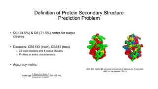
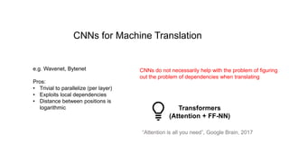
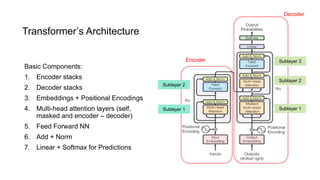
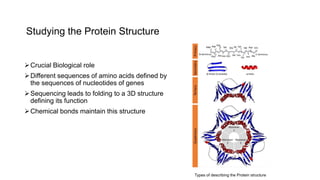
1) The document discusses using a Transformer model for protein secondary structure prediction (PSSP). Transformers use self-attention and avoid issues with long-term dependencies that RNNs face. 2) Several experiments were conducted to determine the best Transformer architecture for PSSP, varying number of layers (N), hidden sizes (d_model), attention heads (h), and other hyperparameters. The best results were around 63-64% accuracy with N=2, d_model=128-256, and h=8. 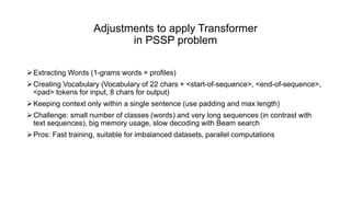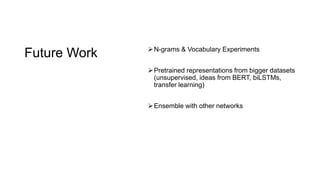3) Future work proposed includes exploring n-gram representations, pretraining on larger datasets, and ensembling with other models.

1. Protein Secondary Structure Prediction using Deep Learning
techniques
National Technical University of Athens
School of Electrical and Computer Engineering
Department of Information Technology and Computers
THESIS
CHRYSOULA KOSMA
Supervisor: Georgios Stamou
Associate Professor NTUA Athens, November 2019

2. Dealing with Biological Sequences
Importance
Different types of problems studied by the genomics group (pathogenicity, species
identification from rRNA sequences, promoter's identification)
Challenges: limited data, long sequences → difficult to process with simple NN
architectures
Approaches: deep CNNs (with dilated convolutions), ideas NLP models (attention layers,
encoder-decoder architectures for sequence prediction)

3. Common Types of biological
sequences
1. DNA seq - Genomics
2. RNA seq - Transcriptomics
3. Protein Seq - Proteomics

4. Dealing with Biological Sequences
Taxonomic hierarchy derives by the whole DNA of an organism.
Shorter sequences - ML approaches.
(Google Brain: A deep learning approach to pattern recognition for
short DNA sequences.)
SPECIES IDENTIFICATION
Chemical bonds between the amino acid residues give proteins their
complex structure.
PROTEIN STRUCTURE PREDICTION

5. Studying the Protein Structure
Crucial Biological role
Different sequences of amino acids defined by
the sequences of nucleotides of genes
Sequencing leads to folding to a 3D structure
defining its function
Chemical bonds maintain this structure
Types of describing the Protein structure

6. Definition of Protein Secondary Structure
Prediction Problem
• Q3 (84.5%) & Q8 (71.5%) codes for output
classes
• Datasets: CB6133 (train), CB513 (test)
o 22 input classes and 8 output classes
o Profiles as extra characteristics
• Accuracy metric:
Average
#Correct chars
sequence length
for all seq
(left) Q3, (right) Q8 secondary structure of spheres for the protein
1AKD in the dataset CB513.

7. State-of-the-art PSSP Q8
Method Accuracy(%)
Ensemble 70.7
Bidirectional GRU with
convolution blocks
69.8
U-Net with convolution blocks 69.2
Temporal convolutional network 68.7
Bidirectional LSTMs with
attention
68.4
Convolutions and Bidirectional
LSTM
67.8
Bidirectional GRUs 67.4
High Quality Protein Q8 Secondary Structure
Prediction by Diverse Neural Network
Architectures, 2018

8. Method Accuracy(%)
2-block CNN† 69.7
2- block EINN† 69.8
2-block CNN∗† 69.8
4-block CNN∗† 70.6
8-block CNN∗† 71.2
12-block CNN∗† 71.5
16-block CNN∗† 71.3
8-block MCNN∗† 71.3
12-block MCNN∗† 71.5
State-of-the-art PSSP Q8
Neural Edit Operations for Biological Sequences, 2018
(left) ConvBlock, (right) Modified ConvBlock
† for data augmentation, * for multitasking

9. Introduction in Neural
Machine Translation
 Input Sequence → Output Sequence (not necessarily of the same length) e.g. speech recognition,
text-to-speech, language modelling
 Need for capturing dependencies within sequences (Context)
Sequence-to-
sequence model
You are awesome Ti si super
You are awesome Ti si superEncoder Decoder
Context

10. Recurrent Neural
Networks
→ The problem of long-term dependencies
Traditional Sequence-to-
sequence architectures

11. LSTMs
Traditional Sequence-to-
sequence architectures
• Sequential computation inhibits parallelization
• No explicit modeling of long and short range dependencies
• Distance between positions is linear

12. Introducing Attention Layers to
RNNs
You are awesome
Ti si super
Encoder
RNN
Hidden
State1
Encoder
RNN
Hidden
State2
Encoder
RNN
Hidden
State3
Hidden
State1
Hidden
State2
Attention
Decoder
RNN
Attention
Decoder
RNN
Attention
Decoder
RNN
Sequence-to-sequence with Attention

13. e.g. Wavenet, Bytenet
Pros:
• Trivial to parallelize (per layer)
• Exploits local dependencies
• Distance between positions is
logarithmic
CNNs for Machine Translation
CNNs do not necessarily help with the problem of figuring
out the problem of dependencies when translating
Transformers
(Attention + FF-NN)
“Attention is all you need”, Google Brain, 2017

14. Transformer’s Architecture
Basic Components:
1. Encoder stacks
2. Decoder stacks
3. Embeddings + Positional Encodings
4. Multi-head attention layers (self,
masked and encoder – decoder)
5. Feed Forward NN
6. Add + Norm
7. Linear + Softmax for Predictions
Encoder
Decoder
Sublayer 1
Sublayer 2
Sublayer 1
Sublayer 2
Sublayer 3

15. Encoder and Decoder stacks

16. Input Vectors
 Word Embeddings:
• Embedding Layer
• Weight matrix W(num_embeddings, embedding_dim)
• Random initialization for the PSSP problem
• Learnable
 Positional Encodings:
• Relative order of words in the sequence
• Added to the word embedding to create the final word representation
• Calculated by the equation:
PE(pos,2i) = sin(pos/10002i/dmodel)
PE(pos,2i+1) = cos(pos/10002i/dmodel)
Vocab size dmodel parameter

17. Self-Attention
trainable
Queries
Keys
Values
query = linear(x)
key = linear(x)
value = linear(x)

18. Self-Attention
Calculation
Attention Q, V, K = softmax
QKT
dk
V
Q: queries matrix
K: keys matrix
V: values matrix
dk: dimension of keys

19. Multi-Head Attention
h: number of Attention heads (h=8 in the paper)

20. Attention Layers
1. Self-Attention (Encoder)
2. Masked Self-Attention (Decoder)
3. Encoder-Decoder Attention
Attention(Q, V, K) = softmax
QKT
dk
V
MultiHead Q, K, V = Concat head1, … , headh WO
headi = Attention(QWi
Q
, KWi
K
, VWi
V
)
Wi
Q
∈ ℝdmodel×dk, Wi
K
∈ ℝdmodel×dk,
Wi
V
∈ ℝdmodel×dv, WO
∈ ℝhdv×dmodel

21. Attention Layers & other details
• Masked Self-Attention (Decoder)
o Masks future positions
• Encoder-Decoder Attention
• Queries come from decoder stack
• Keys and Values from the output of the
Encoder Stack
• FFN(x) = max(0, xW1 + b1)W2 +
b2
• Residual Connections & Layer
Normalization

22. Training Process
• Input = Embeddings + positional encodings
• Linear & Softmax for output
• Adam Optimizer with variable learning rate
• Label Smoothing option
• Cross entropy for loss function

23. Translation
• Process:
1. Creating the encodings of test set using the checkpoint (run Encoder)
2. Run decoder
• Start with <start-of_sentence> and decode
• Feed the previous predictions into the decoder
• Decode until an <end-of-sentence> is produced
• Two decoding techniques:
1. Greedy Decoding
2. Beam Search (keep k possible predictions for each word)

24. Adjustments to apply Transformer
in PSSP problem
Extracting Words (1-grams words + profiles)
Creating Vocabulary (Vocabulary of 22 chars + <start-of-sequence>, <end-of-sequence>,
<pad> tokens for input, 8 chars for output)
Keeping context only within a single sentence (use padding and max length)
Challenge: small number of classes (words) and very long sequences (in contrast with
text sequences), big memory usage, slow decoding with Beam search
Pros: Fast training, suitable for imbalanced datasets, parallel computations

25. Experiments and Results
Number of Parameters to tune:
• N, h
• d_model, d_k, d_v, d_inner_hid
• batch_size, epochs, dropout
• label_smoothing(True/False, 𝑒𝑙𝑠),
learning rate
• Adam’s Optimizer (3 parameters)
Organizing Experiments:
1. Random Search:
• epoch = 200
• patience = 10, 20
• warmup_steps = 4000
• lrate = dmodel
−0.5
∙
min(step_num−0.5, step_num ∙
warmup_steps−1.5
)
• β1 = 0.9, β2 = 0.98, e = 10−9
(Adam)
• els = 0.1 for Label smoothing
2. Tests for specific combinations
15
total

26. Experiments and Results
1. 1st set: h = 8,16, d_inner_hid = 4 ∙ d_model, d_k = d_v = d_model/4, dropout = 0.01,0.1,0.6, N =
1,2,3,4,5,6, d_model = 32,64,128,256,512, label_smoothing = True, False,batch_size = 10,18.
2. 2nd set: h = 8, d_inner_hid = 4 ∙ d_model, d_k = d_v = d_model/2, dropout = 0.01,0.1, N = 1,2,
d_model = 32,64,128,256,512, label_smoothing = False, batch_size = 20.
 Early stopping technique was applied with specific patience regarding validation loss

27. N d_model d_k,d_v d_inner h dropout LabelS.
acc(%),
beam_s=1
acc(%),
beam_s=5
acc(%),
beam_s=10
1 32 8 128 8 0.1 False 60.17 ↑ 61.11 60.92
2 128 32 512 8 0.1 False 44.55 49.93 49.56
1 256 64 1,024 8 0.01 False 59.4 ↑ 60.53 60.41
1 64 16 256 8 0.01 False 59.19 60.80 60.76
1 64 16 256 8 0.01 False 61.27 ↑ 62.49 62.4
1 128 32 512 8 0.01 False 58.22 59.35 58.93
1 128 32 512 8 0.1 False 61.03 ↑ 62.12 62.0
1 512 128 2,048 8 0.01 False 58.24↑ 60.1 59.74
Results (1st set) with increased batch size
ℎ = 8, 𝑏𝑎𝑡𝑐ℎ_𝑠𝑖𝑧𝑒 = 18, 𝑝𝑎𝑡𝑖𝑒𝑛𝑐𝑒 = 10

28. N d_model d_k,d_v d_inner h dropout LabelS. acc(%), beam_s=1 acc(%), beam_s=5
1 512 256 2,048 8 0.1 False 58.39 60.12
1 512 256 2,048 8 0.01 False 58.36 59.39
1 256 128 1,024 8 0.1 False 58.36 58.87
1 256 128 1,024 8 0.01 False 57.07 59.21
1 128 64 512 8 0.1 False 56.81 58.86
1 128 64 512 8 0.01 False 56.75 58.39
1 64 32 256 8 0.1 False 58.96 60.6
1 64 32 256 8 0.01 False 59.35 60.55
1 32 16 128 8 0.1 False 62.03 63.04
1 32 16 128 8 0.01 False 59.54 62.72
Results (2nd set)
ℎ = 8, 𝑏𝑎𝑡𝑐ℎ_𝑠𝑖𝑧𝑒 = 20, 𝑝𝑎𝑡𝑖𝑒𝑛𝑐𝑒 = 20

29. N d_model d_k,d_v d_inner h dropout LabelS.
acc(%),
beam_s=5
acc(%),
beam_s=10
2 512 256 2,048 8 0.1 False 33.63 29.77
2 512 256 2,048 8 0.01 False 29.36 28.24
2 256 128 1,024 8 0.1 False 60.43 60.51
2 256 128 1,024 8 0.01 False 64.22 64.36
2 128 64 512 8 0.1 False 63.30 63.22
2 128 64 512 8 0.01 False 62.34 62.55
2 64 32 256 8 0.1 False 62.85 62.59
2 64 32 256 8 0.01 False 58.96 58.45
2 32 16 128 8 0.1 False 63.7 63.5
Best Results (2nd set)
ℎ = 8, 𝑏𝑎𝑡𝑐ℎ_𝑠𝑖𝑧𝑒 = 20, 𝑝𝑎𝑡𝑖𝑒𝑛𝑐𝑒 = 20

30. Conclusions
• Overfitting for N ≥ 3 encoder and decoder stacks (lack of
data?)
• Smooth training for N = 1,2 stacks (training takes ~40-
60min, less than 100 epochs)
• Large input spaces capture better dependencies
(dmodel, d_k = d_v = d_model/2)
• h = 8 attention heads handle better the long input
sequences (less are not sufficient)
• Small dropout rate for small networks helps training
• Decoding with beam search is slow (as the beam_size
increases, beam_size = 10 takes 1hour)
• Label smoothing didn’t show improvements
• Larger batch_size (~20) helps training but there are
memory limits

31. Future Work N-grams & Vocabulary Experiments
Pretrained representations from bigger datasets
(unsupervised, ideas from BERT, biLSTMs,
transfer learning)
Ensemble with other networks