Download to read offline


![1.2 Objectives
In this section we outline the objectives of this thesis.
• To develop an optimization model for the transmission of multicast applications. The
main objective function in the development of the model is to minimize the maximum link
utilization. The solution obtained by this model can distribute traffic between multiple
trees by using a multi-path scheme from the ingress node to each egress node. Using this
scheme it is possible to transmit the information through more than one path between
ingress node and egress node. For the multicast case, which is the topic of this thesis, it
would consist in transmitting information flow through more than one tree. The
contribution is that the current multicast routing protocols such as DVMRP [WAI88]
[PUS00], MOSPF [MOY94], PIM-DM [DEE98], PIM-SM [EST98], CBT [BAL97] [BAL97a]
and BGMP [THA00], transmit the information through just one tree.
• To broaden the possibilities of the above model with other objectives (total hop count,
end-to-end delay and bandwidth consumption). As this model uses a load-balancing
technique it is possible, in this case, that very long paths can be found.
• To make the model appropriate for dynamic connections. As in multicast
transmissions, egress nodes can go in and out of the connection during the life-time
connection, another objective is to present a new model solving the problem of dynamic
nodes.
• To specify the way of creating paths between ingress nodes and egress ones by using
MPLS technology, that is Label Switched Paths (LSPs) based on solutions found with the
analytical model previously proposed.
• To propose a taxonomy to classify related works and this thesis contributions.
• To define a generalized model in order to be able to consider and cover most of different
models and their objectives, found in bibliographical reviews.
• To find a solution to the problem by using MOEA.
• To analyze the validity of the proposed models through simulations.
3](https://image.slidesharecdn.com/programacionmultiobjetivo-121118123824-phpapp02/85/Programacion-multiobjetivo-23-320.jpg)


![user(s) of the network. QoS requirements of a specific flow can be specified in terms of packet
loss probability, bandwidth, end-to-end delay, reliability, etc. The customers of the network
may agree with the service providers on the QoS requirements via Service Level Agreements
(SLAs).
Quality of Services, in its simplest form, is defined as the mechanism that fulfils the
requirements of the applications in a network, that is, one or some elements of the network
that can guarantee, to a certain extent, that the traffic needs are fulfilled. All the layers of the
network are involved in these elements of quality of service. QoS works by assigning priorities
according to network traffic needs, and by managing in this way the network bandwidth
[WAN01].
The following parameters have been widely used to describe the requirements of Quality of
Service:
• Minimum bandwidth: the minimum amount of bandwidth requested by an application
flow. The time interval for measuring the bandwidth must be specified because
different intervals may give different results. The algorithms of packet scheduling
guarantee bandwidth assignment.
• Delay: Delay requesting can be specified as the average delay or the delay in the worst
case. The delay experimented by a package consists of three components: propagation
delay, transmission delay, and queue delay. Propagation delay is caused by light speed
and is directly related to the distance. Transmission delay is the time taken to send a
package across a link. Queue delay is the time that packages have to wait.
• Delay jitter: a delay jitter request can be said to specify the maximum difference
between the longest delay and the shortest one experienced by the packages. This
should not be longer than the transmission in the worst case and the delay in a queue.
• Loss rate: This is the rate of lost packages and the total amount of transmitted
packages. Package loss in Internet is often caused by congestion. By assigning enough
bandwidth and buffers for traffic flow these losses can be prevented.
One of the causes of low performance in networks is congestion, which is the inability to
transmit a volume of information with the established capacities for a particular equipment or
network.
8](https://image.slidesharecdn.com/programacionmultiobjetivo-121118123824-phpapp02/85/Programacion-multiobjetivo-28-320.jpg)

![Traffic engineering in MPLS networks is similar to those arising in Asynchronous Transfer
Mode (ATM) networks. To bring guaranteed QoS (lacking in connectionless IP networks),
MPLS provides connection-oriented capabilities, as in ATM networks. LSPs coincide with the
circuit-switched paths in ATM networks [CER04].
Several advantages of using multipath routing are discussed in [CHE01] and [IZM02]. Links
do not get overused and therefore do not get congested, and so they have the potential to
aggregate bandwidth, allowing a network to support a higher data transfer than is possible
with any single path. Several paths can be used as backup paths for one primary path when
paths are configured maximally disjoint. Each working path is protected by an alternative
disjoint path. If the primary path goes down, alternative paths can quickly be deployed.
Therefore, load balancing emerges as a fast response path protection mechanism.
Furthermore, some authors have expanded this idea by proposing to split each flow into
multiple subflows in order to achieve better load balancing [DON04], [DON03], [KIM04] and
[KIM02]. The flow splitting approach can be used for the protection path. Splitting the
working path has the advantage of reducing the amount to be protected [IZM02].
The per-packet overhead therefore has to be small, and to reduce implementation complexity,
the system should keep no or little state information. Second, traffic–splitting schemes
produce stable traffic distribution across multiple outgoing links with minimum fluctuation.
Last but not least, the traffic–splitting algorithms must maintain per-flow packet ordering.
Packet misordering within a TCP flow can produce a false congestion signal and cause
unnecessary throughput degradation.
Simple schemes for traffic splitting are based on packet–by–packet round robin results in low
overheads and good performance. They may, however, cause per–flow ordering. Sequence
numbers or state may be added to reordering, but these additional mechanisms drastically
increase complexity, and in many cases they only work in point–to-point links.
Hashing based traffic–splitting algorithms are stateless and easy to implement, particularly
with hardware assistance. For hash functions that use any combination of the five-tuple as
input, per–flow ordering can be preserved; all packets within the same TCP flow have the
same five–tuple, and so the output of the hash function with the five–tuple as input should
always be the same.
12](https://image.slidesharecdn.com/programacionmultiobjetivo-121118123824-phpapp02/85/Programacion-multiobjetivo-32-320.jpg)
![A simple method to divide the input traffic is on a per-packet basis, for example in a round-
robin fashion. However, this method could result in excessive packet reordering and is not
recommended in practice. [VIL99] tries to balance the load among multiple LSPs according to
the loading of each path. In MPLS networks [ROS01] multiple paths can be used to forward
packets belonging to the same “forwarding equivalent class” (FEC) by explicit routing. Once
the explicit path is computed, the signaling protocol Constraint-Based Routing Label
Distribution Protocol (CR-LDP) [ASH02] [ASH02a] or Resource Reservation Protocol with
Traffic Engineering extension (RSVP-TE) [AWD01] is responsible for establishing forwarding
state and reserve resources along the route in both last protocols. How the load is distributed
between a set of alternate paths is determined by the amount of number space from a hash
computation that is allocated to each path. Effective use of load balancing requires good traffic
distribution schemes. In [CAO00] the performance of several hashing schemes for distributing
traffic between multiple links while preserving the order of packets within a flow is studied.
Although hashing-based load balancing schemes have been proposed in the past, [CAO00] is
the first comprehensive study of how the schemes perform using real traffic traces. The
current configurations in computer networks provide an opportunity for dispersing traffic over
multiple paths to decrease congestion. In this work dispersion involves (1) splitting and (2)
forwarding the resulting portions of aggregate traffic along alternate paths. The authors
concentrate on (1), methods that allow a network node to subdivide aggregate traffic, and they
offer a number of traffic splitting policies which divide traffic aggregates according to the
desired fractions of the aggregate rate. Their methods are based on semi-consistent hashing of
packets to hash regions as well as prefix-based classification [CAO00a]. The analysis of
hashing methods is out of these thesis topics.
2.2.3 Load Balancing of Unicast Flows
In the Unicast case the network is modeled as a directed graph G = ( N , E ) , where N is the set
of nodes and E is the set of links. We use n to denote the number of network nodes, i.e. n = N .
Among the nodes, we have a source s ∈ N (ingress node) and a destination t ∈ N (egress
node). Let (i , j ) ∈ E be the link from node i to node j. Let f ∈ F be any unicast flow, where
F is the flow set. We denote the number of flows by |F|. Let X ijf be the fraction of flow f
assigned to link (i,j). The problem solution, X ijf variables, provides optimum flow values. Let cij
be the capacity of each link (i,j). Let bwf be the traffic demand of a flow f. The problem of
minimizing |F| unicast flows from ingress node s to egress node t is formulated as follows
[WAN01]:
13](https://image.slidesharecdn.com/programacionmultiobjetivo-121118123824-phpapp02/85/Programacion-multiobjetivo-33-320.jpg)

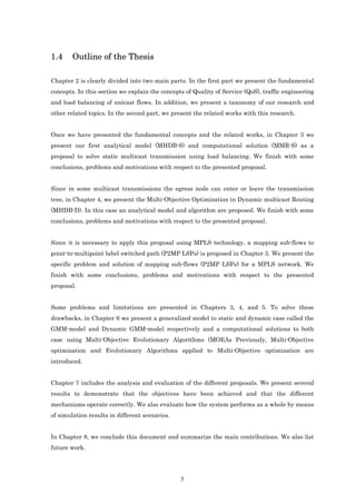
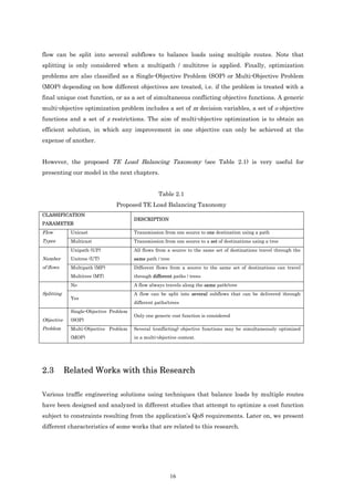
![X = 0 .5
LSP1 24 2
X 1 2 = 0 .5 2
1 4
1 4
LSP 2
3 X 13 = 0.5 3
X 34 = 0.5
Fig 2.2. 1st Transmission Path in Unicast Fig 2.3. 2nd Transmission Path in Unicast
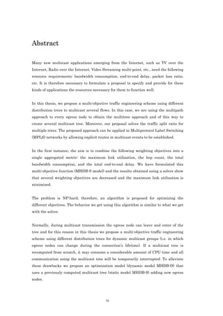
Constraint (2.4) ensures that the total flow coming from an egress node t of flow f is 1.
Constraint (2.5) ensures that for any intermediate node that is different from the ingress node
(i ≠ s) and egress nodes (i ≠ t ) , the sum of its output flows minus the input flows with a
f
( f f
)( f
destination at egress node t of flow f is 0. i.e. x 24 − x12 = 0 , x 34 − x13 = 0 . )
Constraint (2.6) is the MLU constraint. The total amount of bandwidth consumed by all the
flows in the link (i,j) must not exceed the maximum utilization (α) per link capacity cij.
Expression (2.7) shows that the X ijf variables must be real numbers between 0 and 1 because
they represent the fraction of each flow that is transmitted. These variables form multiple
trees to transport a multicast flow. The demand between the ingress node and egress node t
may be split between multiple routes. When the problem is solved without load balancing, this
variable is only able to take values 0 and 1, which show, respectively, whether or not the link
(i,j) is being used to carry information to egress node t.
In [WAN01] and [LEE02] a solution for unicast transmission has been presented.
2.2.4 Taxonomy
In this section we present a taxonomy that helps to clarify and better understand the problems
associated with multicast transmission, load balancing, traffic splitting and multi-objective
optimization.
First, the taxonomy considers the flow type when classifying reviewed works into a traditional
unicast flow type and a more general multicast flow type. Second, it categorizes load balancing
techniques considering the number of paths/trees employed. For instance, if different flows
going from a given source to the same set of destinations can be delivered (or not) through
different paths/trees, a flow could use a path/tree while another flow could go through a
different path/tree, both leave a given source node and go to the same set of destinations.
Moreover, load balancing techniques are classified in relation to splitting, i.e. whether a given
15](https://image.slidesharecdn.com/programacionmultiobjetivo-121118123824-phpapp02/85/Programacion-multiobjetivo-35-320.jpg)
![In [RAO98] the authors consider two generic routing algorithms that plan multipaths
consisting of possibly overlapping paths. Therefore, bandwidth can be reserved and
guaranteed once it is reserved in the links. The first problem deals with transmitting a
message of finite length from the ingress node to the egress node within r units of time. A
polynomial-time algorithm is proposed and the results of a simulation are used to illustrate its
applicability. The second problem deals with transmitting a sequence of some units at such a
rate that the maximum time difference between the two units received out of order is limited.
The authors show that this second problem is computationally intractable, and propose a
polynomial-time approximation algorithm. Therefore, a Quality of Service Routing (QoSR)
routing along multiple paths under a time constraint is proposed when the bandwidth can be
reserved.
[RAO98] Characteristics
Reference Year Objective functions Constraints Taxonomy Heuristic
Flow Type: Unicast
Delay Number of flows: Multipath Ford-Fulkason
[RAO98] 1998 Bandwidth
Splitting: No method
Single-Objective
Objective problem:
Problem
In [ABO98] the authors propose a fuzzy optimization model for routing in Broadband
Integrated Service Digital Network (B-ISDN) networks. The challenge of the proposed model is
to find routes for flows using paths that are not hideously expensive, fulfill the required QoS
and do not penalize the other flows that already exist or that are expected to arrive in the
network. The model is analyzed in terms of performance in different routing scenarios. The
authors obtained good improvements in performance compared with the traditional single
metric routing techniques (number of hops or delay based routing). This improvement was
achieved while maintaining a sufficiently low processing overhead. Throughput was increased
and the probability of congestion was decreased by balancing the load over all the network
links.
[ABO98] Characteristics
Reference Year Objective functions Constraints Taxonomy Heuristic
Flow Type: Unicast
Link Utilization
Hop Count Bandwidth Number of flows: Multipath Fuzzy logic,
[ABO98] 1998
Delay Splitting: No Weighted Sum
Single-Objective
Objective problem:
Problem
17](https://image.slidesharecdn.com/programacionmultiobjetivo-121118123824-phpapp02/85/Programacion-multiobjetivo-37-320.jpg)
![In [FOR02] the authors propose optimizing the weight setting based on the projected demands.
They show that optimizing the weight settings for a given set of demands is NP-hard, so they
resort to a local search heuristic. They found weight settings that performed to within a few
percent of the optimal general routing, where the flow for each demand is optimally
distributed over all paths between the source and destination. This contrasts with the common
belief that Open Shortest Path First (OSPF) routing leads to congestion and shows that for the
network and demand matrix studied it is not possible to get substantially better load
balancing by switching to the proposed more flexible MPLS technologies.
[FOR02] Characteristics
Reference Year Objective functions Constraints Taxonomy Heuristic
Flow Type: Unicast
Number of flows: Multipath Linear
Link Utilization Bandwidth
[FOR02] 2002 programming and
Splitting: No shortest path
Single-Objective
Objective problem:
Problem
In [SRI03] the authors propose an approach that remedies two main difficulties in optimal
routing. The first is that these protocols use shortest path routing with destination based
forwarding. The second is that when the protocols generate multiple equal cost paths for a
given destination routing prefix, the underlying forwarding mechanism balances the load
across these paths by splitting traffic equally between the corresponding set of next hops.
These added constraints make it difficult or impossible to achieve optimal traffic engineering
link loads. It builds links by taking advantage of the fact that shortest paths can be used to
achieve optimal link loads, but it is compatible with both destination based forwarding and
even splitting of traffic over equal cost paths. Compatibility with destination based forwarding
can be achieved through a very minor extension to the result obtained in [WAN01a], simply by
taking advantage of a property of shortest paths and readjusting traffic splitting ratios
accordingly. Accommodating the constraint of splitting traffic evenly across multiple shortest
paths is a more challenging task. The solution we propose stems from the fact that current day
routers have thousands of route entries (destination routing prefixes) in their routing table.
Instead of changing the forwarding mechanism responsible for distributing traffic across equal
cost paths, we plan to control the actual (sub)set of shortest paths (next hops) assigned to
routing prefix entries in a router’s forwarding table(s).
18](https://image.slidesharecdn.com/programacionmultiobjetivo-121118123824-phpapp02/85/Programacion-multiobjetivo-38-320.jpg)
![[SRI03] Characteristics
Reference Year Objective functions Constraints Taxonomy Heuristic
Flow Type: Unicast
Link Utilization Number of flows: Multipath Linear
Bandwidth
[SRI03] 2003 Bandwidth programming and
Splitting: No shortest path
Single-Objective
Objective problem:
Problem
In [SON03] the author proposes an adaptive multipath traffic engineering mechanism called
Load Distribution over Multipath (LDM). The main goal of LDM is to enhance the network
utilization as well as the network performance by adaptively splitting the traffic load among
multiple paths. LDM takes a pure dynamic approach that does not require any previous traffic
load statistics. Routing decisions are made at the flow level and traffic proportioning reflects
both the length and the load of a path. Moreover, LDM dynamically selects a few good Label
Switched Paths (LSPs) according to the state of the entire network.
[SON03] Characteristics
Reference Year Objective functions Constraints Taxonomy Heuristic
Flow Type: Unicast
(Linear) multi-
Hop Count Number of flows: Multipath
Hop Count commodity
[SON03] 2003 Bandwidth
Splitting: No network flow
Single-Objective problem
Objective problem:
Problem
In [VUT00] the authors propose a traffic engineering solution that adapts the minimum-delay
routing to the backbone networks for a given long-term traffic matrix. This solution is practical
and is suitable to implement in a Differential Services framework. In addition, they introduce
a simple scalable packet forwarding technique that distinguishes between datagram and
traffic that requires in-order delivery and forwards them accordingly and efficiently.
[VUT00] Characteristics
Reference Year Objective functions Constraints Taxonomy Heuristic
Flow Type: Unicast
Delay Bandwidth Number of flows: Multipath Non linear
[VUT00] 2000
Splitting: Yes programming
Single-Objective
Objective problem:
Problem
In [CHE01] the authors propose an algorithm to carry out the unicast transmission of
applications requiring minimum bandwidth through multiple routes. The algorithm consists of
19](https://image.slidesharecdn.com/programacionmultiobjetivo-121118123824-phpapp02/85/Programacion-multiobjetivo-39-320.jpg)
![five steps: a) the multipath P set is initialized as empty, b) the maximum flow graph is
obtained, c) the shortest route from the ingress node to the egress node is obtained, d) the
bandwidth consumption obtained in the maximum flow of step b is decreased, and e) step (d) is
repeated until the required bandwidth for transmission is reached. The results presented show
very similar end-to-end delay values to those obtained independently whether the load
balancing is applied or not. However, link utilization is improved when load balancing is
applied.
[CHE01] Characteristics
Reference Year Objective functions Constraints Taxonomy Heuristic
Flow Type: Unicast
Delay Bandwidth Number of flows: Multipath Max-flow and
[CHE01] 2001
Splitting: Yes shortest path
Single-Objective
Objective problem:
Problem
In [WAN01a] the authors present a multi-objective optimization scheme to transport unicast
flows. In this scheme they consider the MLU (α) and the selection of best routes based on the
flow assigned to each link. In this paper the authors consider a new approach that
accomplishes traffic engineering objectives without full mesh overlaying. Instead of overlaying
IP routing over the logical virtual network traffic engineering objectives such as balancing
traffic distribution are achieved by manipulating link metrics for IP routing protocols such as
OSPF. In this paper, they present a formal analysis of the integrated approach, and propose a
systematic method for deriving the link metrics that convert a set of optimal routes for traffic
demands into the shortest path with respect to the link weights that pass through them. The
link weights can be calculated by solving the dual of a linear programming formulation.
[WAN01a] Characteristics
Reference Year Objective functions Constraints Taxonomy Heuristic
Flow Type: Unicast
Link Utilization Linear
Bandwidth Bandwidth Number of flows: Multipath
[WAN01a] 2001 Programming,
Flow assignation Splitting: Yes Weighted Sum
Single-Objective
Objective problem:
Problem
In [LEE02] the authors propose a method for transporting unicast flows. The constraint of a
maximum number of hops is added to the minimization of the MLU (α). Moreover, the traffic is
divided between multiple routes in a discrete way. This division simplifies implementing the
solution. The behavior of five approaches are analyzed: Shortest path based on non-
20](https://image.slidesharecdn.com/programacionmultiobjetivo-121118123824-phpapp02/85/Programacion-multiobjetivo-40-320.jpg)
![bifurcation, Equal Cost Multiple Paths (ECMP), Traffic bifurcation, H Hop-constrained traffic
bifurcation and H Hop-constrained traffic bifurcation with node affinity. Through the
approaches of Hop-constrained traffic bifurcation, a minimum value of the MLU (α) is
obtained.
[LEE02] Characteristics
Reference Year Objective functions Constraints Taxonomy Heuristic
Flow Type: Unicast
Number of flows: Multipath Mixed-integer
Hop Count
[LEE02] 2002 Link Utilization
Bandwidth Splitting: Yes programming
Single-Objective
Objective problem:
Problem
In [ABR02] the authors propose an intra-domain routing algorithm based on multi-commodity
flow optimization which allows load sensitive forwarding over multiple paths. It is not
constrained by weight-tuning of the legacy routing protocols, such as OSPF, and it does not
require a totally new forwarding mechanism, such as MPLS. These characteristics are
accomplished by aggregating the traffic flows destined for the same egress into one commodity
in the optimization and using a hash based forwarding mechanism. The aggregation also
reduces computational complexity, which makes the algorithm feasible for on-line load
balancing. Another contribution is the optimization objective function, which allows precise
tuning of the tradeoff between load balancing and total network efficiency.
[ABR02] Characteristics
Reference Year Objective functions Constraints Taxonomy Heuristic
Flow Type : Unicast
(Linear) multi-
Link Utilization Number of flows: Multipath commodity
[ABR02] 2002
Splitting: Yes network flow
Single-Objective problem
Objective problem:
Problem
In [CHO03] the authors propose two multi-path constraint based routing algorithms for
Internet traffic engineering using MPLS. In a normal Constraint-based Shortest Path First
(CSPF) routing algorithm, there is a high probability that it cannot find a feasible path
through networks for a large bandwidth constraint. This is one of the most significant
constraints of traffic engineering. The proposed algorithms can divide the bandwidth
constraint into two or more sub constraints and find a constrained path for each sub
constraint, providing there is no single path satisfying the whole constraint. Extensive
21](https://image.slidesharecdn.com/programacionmultiobjetivo-121118123824-phpapp02/85/Programacion-multiobjetivo-41-320.jpg)
![simulations show that they enhance the success probability of path setup and the utilization of
network resources.
[CHO03] Characteristics
Reference Year Objective functions Constraints Taxonomy Heuristic
Flow Type: Unicast
Bandwidth Bandwidth Number of flows: Multipath Max-flow and
[CHO03] 2003
Subflows Splitting: Yes Shortest Path
Single-Objective
Objective problem:
Problem
In [CET04] the authors introduce Opportunistic Multipath Scheduling (OMS), a technique for
exploiting short term variations in path quality to minimize delay, while simultaneously
ensuring that the splitting rules dictated by the routing protocol are fulfilled. In particular,
OMS uses measured path conditions in time scales of up to several seconds to
opportunistically favor low-latency high-throughput paths. However, a naive policy that
always selects the highest quality path would violate the routing protocol’s path weights and
potentially lead to oscillation. Consequently, OMS ensures that over longer time scales
relevant for traffic management policies, traffic is split according to the ratios determined by
the routing protocol. A model of OMS is developed and an asymptotic lower bound on the
performance of OMS as a function of path conditions (mean, variance, and Hurst parameter)
for self-similar traffic is derived.
[CET04] Characteristics
Reference Year Objective functions Constraints Taxonomy Heuristic
Flow Type: Unicast
Delay Number of flows: Multipath
Bandwidth Scheduling
[CET04] 2004 Queue Size
Splitting: Yes Algorithm
Single-Objective
Objective problem:
Problem
In [KIM04] the author suggests a method to improve network performance by appropriately
distributing traffic in accordance with the state of the paths in a dynamic traffic pattern
occurring in a short time in a multipath environment. TE using an Adaptive Multipath-
forwarding (TEAM) is a traffic engineering (TE) algorithm that aims to improve network
performance by properly distributing traffic in dynamic traffic patterns occurring in a short
time scale. This method monitors the state of the paths by using a probe packet in the ingress
node of the network, and computes the cost of the paths with monitored values. Path cost
consists of weights given in the paths, such as packet delay and loss rate, the number of hops
22](https://image.slidesharecdn.com/programacionmultiobjetivo-121118123824-phpapp02/85/Programacion-multiobjetivo-42-320.jpg)
![and the number of LSPs. This enables it to adapt to the state of the network without a sudden
change by tracing neighboring solutions from an existing solution. Therefore, it can be seen
that network performance is improved when the total cost of paths of the whole network are
minimized. In addition, by distributing traffic into each interface using a table-based hashing
method, the problem of ordering packets is solved.
[KIM04] Characteristics
Reference Year Objective functions Constraints Taxonomy Heuristic
Flow Type: Unicast
Hop Count
Delay Number of flows: Multipath
[KIM04] 2004 Flow assignation Shortest path
Number of LSPs Splitting: Yes
Single-Objective
Objective problem:
Problem
In [SEO02] the authors propose non-bifurcation and bifurcation methods to transport
multicast flows with hop-count constraints. When analyzing results and simulations, they only
consider the non-bifurcation methods. The constraint of consumption bandwidth is added to
the constraints considered in [RAO98]. In [LEE02] a heuristic is proposed. The proposed
algorithm consists of two parts: 1) modifying the original graph to the hop-count constrained
version, 2) finding a multicast tree to minimize the MLU (α).
[SEO02] Characteristics
Reference Year Objective functions Constraints Taxonomy Heuristic
Flow Type: Multicast
Link Utilization Hop Count Number of flows: Unitree Mixed-integer
[SEO02] 2002 Bandwidth Bandwidth programming,
Subflows Splitting: Not Applicable Weighted Sum
Single-Objective
Objective problem:
Problem
In [ROY02] the authors propose a new multicast tree selection algorithm based on a non-
dominated sorting technique of a genetic algorithm to simultaneously optimize multiple QoS
parameters. Simulation results demonstrate that the proposed algorithm is capable of
obtaining a set of QoS-based near optimal, non-dominated multicast routes within a few
iterations. In this paper, the authors use a Non-dominated Sorting based Genetic Algorithm
(NSGA) technique to develop an efficient algorithm which determines multicast routes on-
demand by simultaneously optimizing end-to-end delay guarantee, bandwidth requirements
and bandwidth utilization without combining them into a single scalar objective function.
23](https://image.slidesharecdn.com/programacionmultiobjetivo-121118123824-phpapp02/85/Programacion-multiobjetivo-43-320.jpg)
![[ROY02] Characteristics
Reference Year Objective functions Constraints Taxonomy Heuristic
Flow Type: Multicast
Delay
Bandwidth Number of flows: Unitree MOEA based on
[ROY02] 2002
Flow assignation Splitting: Not Applicable NSGA
Multiple-Objective
Objective problem:
Problem
In [CUI03a] the authors propose algorithm MEFPA (Multi-constrained Energy Function based
Precomputation Algorithm) for a multi-constrained QoSR problem based on analyzing linear
energy functions (LEF). They assume that each node s in the network maintains a consistent
copy of the global network state information. This algorithm fulfills each QoS metric to b
degrees. It then computes B
(B = C k −1
b+ k −2 ) coefficient vectors that are uniformly distributed in
the k-dimensional QoS metric space, and constructs one LEF for each coefficient vector. Then
based on each LEF, node s uses Dijkstra's algorithm to calculate a least energy tree rooted by s
and a part of the QoS routing table. Finally, s combines the B parts of the routing table to form
the complete QoS routing table it maintains. For distributed routing, for a path from s to t, in
addition to the destination t and k weights, the QoS routing table only needs to save the next
hop of each path. For source routing, the end-to-end path from s to t along the least energy
tree should be saved in the routing table. Therefore, when a QoS connection request arrives, it
can be routed by looking up a feasible path satisfying the QoS constraints in the routing table.
[CIU03a] Characteristics
Reference Year Objective functions Constraints Taxonomy Heuristic
Flow Type: Multicast
Hop Count
Delay Number of flows: Multitree
[CUI03a] 2003 Cost Shortest Path Tree
Bandwidth Splitting: No
Subflows
Single-Objective
Objective problem:
Problem
In [DON03] we presented several static models which are analyzed by comparing some
particular one-objective optimization functions with the multi-objective optimization function.
24](https://image.slidesharecdn.com/programacionmultiobjetivo-121118123824-phpapp02/85/Programacion-multiobjetivo-44-320.jpg)
![[DON03] Characteristics
Reference Year Objective functions Constraints Taxonomy Heuristic
Flow Type: Multicast Non Linear
Link Utilization
Hop Count Number of flows: Multitree programming,
Bandwidth
[DON03] 2003 Delay max-flow and
Subflows Splitting: Yes
Bandwidth shortest path tree,
Single-Objective Weighted Sum
Objective problem:
Problem
In addition, some master or doctoral theses have worked in the same area, for example the
thesis [CER04] focuses on the multi-objective optimization of Label Switched Path design
problem in MPLS networks. Minimal routing cost, optimal load-balance in the network, and
minimal splitting of traffic form the objectives. The problem is formulated as a zero-one mixed
integer program and aims at exploring the trade-offs among the objectives. The integer
constraints make the problem NP-hard. In this thesis first both the exact and heuristic multi-
objective optimization approaches are discussed, and then a heuristic framework based on
simulated annealing is developed to give a solution to this proposal.
[CER04] Characteristics
Reference Year Objective functions Constraints Taxonomy Heuristic
Flow Type: Unicast
Cost
Link Utilization Bandwidth Number of flows: Multipath Simulated
[CER04] 2004
Splitting (LSPs) Splitting: Yes Annealing
Multi-Objective
Objective problem:
Problem
While [RAO98], [ABO98], [SRI03], [FOR02] and [SON03] consider unicast flow, in [CHE01],
[WAN01a], [LEE02], [CHO03], [ABR02], [CET04] and [VUT00] this unicast flow is split, and
in [SEO02], [ROY02] and [CUI03a] the flow is multicast but not split, thus our proposal solves
the traffic split ratio for multicast flows. The major differences between our work and the other
multicast works are:
• First, from an objectives and function point of view, we propose a multi-objective
scheme to solve the optimal multicast routing problem with some constraints, while
[ROY02] and [CUI03] propose a scheme without constraints.
• Second, in relation to how many trees are used, we propose a multitree scheme to
optimize resource utilization of the network, while [SEO02] and [ROY02] only propose
one tree to transmit the flow information.
25](https://image.slidesharecdn.com/programacionmultiobjetivo-121118123824-phpapp02/85/Programacion-multiobjetivo-45-320.jpg)
![• Third, in relation to traffic splitting, we propose that the traffic split can transmit the
multicast flow information through load balancing using several trees for the same
flow, while [SEO02], [ROY02] and [CUI03a] do not propose this characteristic.
It should be noted that the proposals in [SON03], [WAN01a], [LEE02], [CHO03], [VUT00],
[KIM04] and [SEO02] can be applied to MPLS networks.
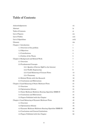
Table 2.2 classifies the papers that could be considered as the most inspired for this research
area. Note that [XIA99] is repeated because it considers unicast and multicast flows. The last
column of Table 2.2 shows the methodologies/heuristics proposed in publications. Clearly, most
publications consider the load balancing problem as a SOP, therefore, they have mainly
proposed using traditional SOP heuristics such as linear programming, shortest path, non-
linear programming and even evolutionary approaches such as genetic algorithms. This last
evolutionary approach is dominant when considering MOPs, where all works surveyed use
some kind of MOEA.
It can be seen that, initially, most papers only considered multipath (and not splitting) for
unicast traffic in a single-objective context. Immediately after, multicast flow was also
considered in the same single-objective context (splitting was still not considered). In the year
2000 papers considering splitting began to appear. Lately, the multiobjective context of the TE
problem has slowly been recognized [ROY02], with an increased number of publications since
2003 (see Table 2.2 in bold for the aims of this thesis).
26](https://image.slidesharecdn.com/programacionmultiobjetivo-121118123824-phpapp02/85/Programacion-multiobjetivo-46-320.jpg)
![Table 2.2
Proposed taxonomy applied to reviewed papers including objective functions, constraints and heuristics
Constraint
Objective functions (OF) Taxonomy
(C)
Flow assignation
Number of LSPs
Link Utilization
Packet Loss
Queue Size
Hop Count
Bandwidth
Bandwidth
Flow Type
Number of
Objective
Heuristic
Hop Count
Splitting
problem
Subflows
Reference
Delay
Delay
flows
Jitter
Cost
Year
[XIA99] 1999 X X X X X X SOP Genetic algorithms, Weighted Sum
UP NA
[KOY04] 2004 X X MOP MOEA
[RAO98] 1998 X X Ford-Fulkason method
[ABO98] 1998 X X X X Fuzzy logic, Weighted Sum
[FOR02] 2002 X X Linear programming and shortest path
No SOP
[SRI03] 2003 X X X Linear programming and shortest path
(Linear) multi-commodity network flow
[SON03] 2003 X X X
problem
[VUT00] 2000 X X Non Linear programming
Unicast
[CHE01] 2001 X X Max-flow and shortest path
[WAN01a] 2001 X X X X MP Linear programming, Weighted Sum
[LEE02] 2002 X X X Mixed-integer programming
(Linear) multi-commodity network flow
[ABR02] 2002 X SOP
Yes problem
[CHO03] 2003 X X X Max-flow and Shortest Path
[CET04] 2004 X X X Scheduling algorithm
[KIM02] 2002
X X X X Shortest Path
[KIM04] 2004
[CER04] 2004 X X X X MOP Simulated Annealing
[XIA99] 1999 X X X X X X Genetic algorithms, Weighted Sum
[LEU98] 1998
[INA99] 1999 X Genetic algorithms
[LI99] 1999
[SUN99] 1999 X X SOP Genetic algorithms
[BAN01] 2001 X X Genetic algorithms, Weighted Sum
Mixed-integer programming, Weighted
[SEO02] 2002 X X X X X UT NA Sum
[ROY02] 2002 X X X MOEA based on NSGA
[CUI03] 2003 X X X X MOEA
[ROY04] 2004 X X X MOEA based on NPGA
MOP
Multicast
[CRI04] 2004 X X MOEA based on SPEA
[CRI04a]
2004 X X X MOEA based on SPEA
[CRI04b]
[CUI03a] 2003 X Shortest Path Tree
[LAY04] 2004 X X X X X SOP Genetic algorithms, Weighted Sum
No
[POM04] 2004 X DIMRO Heuristic
[FAB04] 2004 X X X X MOP MOEA based on NSGA
[DON04] 2004
MT
[DON03] 2003
Non-linear programming, max-flow and
[FAB04a] 2004 X X X X X X SOP
Yes shortest path tree, Weighted Sum
[DON04a] 2004
[DON04b] 2004
[BAR04] 2004 X X X X X X X X X X MOP MOEA based on SPEA
UP: Unipath UT: Unitree SOP: Single-Objective Problem
NA: Not Applicable
MOP: Multi-Objective Problem
MP: Multipath MT: Multitree
27](https://image.slidesharecdn.com/programacionmultiobjetivo-121118123824-phpapp02/85/Programacion-multiobjetivo-47-320.jpg)
![TE Load Balancing Taxonomy proposed (see Table 2.1) could be extended with other kind of
concepts like whether the connections are static or dynamic. All works presented previously
(Table 2.2) consider static case. With respect to the dynamic case, some works have been
realized.
One of the important distinctions between unicast and multicast connections is the possibility
of connection dynamics. Now, two categories of multicast routing algorithms, static and
dynamic are identified. If the network topology does not change and that group membership is
fixed during a session, static algorithm is sufficient. However, in a real network environment,
network links and nodes can fail (or be removed) or be recovered (or be added) frequently. In
addition, the group membership can change dynamically during a multicast session. It is
essential to design efficient dynamic multicast routing algorithm operating under dynamic
network environment. This variability adds further complexity to the already difficult problem
of traffic engineering. This kind of problem is known as a dynamic Steiner tree problem
[IM95]. The main different between the static and dynamic cas in multicast transmission is
that in the static case, the group of egress nodes is fixed during set up and the identities of all
egress nodes are available simultaneously. Once a static group has been established,
individual membership remains unmodified until it is discarded. Paths from the ingress node
to all egress nodes are computed at the same time. In the dynamic case, the group of egress
nodes can change during the connection and the identities of the egress nodes are revealed one
by one. Note that the dynamic problem can be reduced to the static problem, if the multicast
tree is recomputed from scratch each time there is a membership change. But, since the
optimal solution obtained is ephemeral, because of the dynamic nature of multicast
connections, the computation of an optimal tree for each membership group change may not be
the best way forward. In the optimization process it is possible to have a solution like the best
path to the new egress node is a direct connection between the ingress node to the egress node.
There are two main design objectives for the dynamic problem. The first is to minimize the
computational complexity required to update a multicast tree. The second is to maintain
routing stability by making minimal changes to the topology of an existing multicast tree,
because multicast sessions cannot tolerate the disturbances and disruptions caused by
excessive changes. As recomputing the multicast tree from scratch is computationally
expensive, it makes sense to compute a near-optimal multicast tree which is minimally
disturbed after each change in the membership group.
28](https://image.slidesharecdn.com/programacionmultiobjetivo-121118123824-phpapp02/85/Programacion-multiobjetivo-48-320.jpg)
![If designing an optimal tree is a complex problem, maintaining this tree optimality after
changes in the membership group may be even more complex. The GREEDY algorithm is a
simple, non-rearrangeable heuristic proposed by Vaxman, with the aim of minimizing the
perturbation to the existing tree. To add a node, i.e. Nnew, to an existing multicast group, a
closest node, i.e. Ntree, already in the tree is chosen and Nnew is attached to the Ntree via the
least cost path. For a delete request, if the node being removed is a leaf node, then the branch
of the tree supporting only that node is pruned. For the case of a nonleaf node, no action is
taken.
In [STR02] present a multicast “life cycle” model that identifies the various issues involved in
a typical multicast session. During the life cycle of a multicast session, three important events
can occur: group dynamics, network dynamics and traffic dynamics. The first two aspects are
concerned with maintaining a good quality (e.g., cost) multicast tree taking into account
member join/leave and changes in the network topology due to link/node failures/additions,
respectively. The third aspect is concerned with flow, congestion, and error control. In this
paper they examine various issues and solutions for managing group dynamics and failure
handling in QoS multicasting, and outline several future research directions.
The dynamic case in multicast transmission can be worked in different ways. In [STR02] the
authors are identifying the different ways, in the Figure 2.4 are shown.
Fig 2.4 Issues in multicast group dynamics
In this thesis, in the dynamic case, we are working with QoS of new members. Te tree type are
build through a combination of shortest path, maximum flow and breadth first search
probabilistic algorithms. We respect to the routing method we are working with multiple path.
29](https://image.slidesharecdn.com/programacionmultiobjetivo-121118123824-phpapp02/85/Programacion-multiobjetivo-49-320.jpg)
![In [RAG99] the authors propose the problem of modifying such a delay-constrained multicast
tree, when new nodes enter or existing members leave the multicast group. They present a
new algorithm called controlled rearrangement for constrained dynamic multicasting
(CRCDM) for on-line updating of delay-constrained multicast trees with the aim of minimizing
the cost of constructing the trees.
In [TRA03] address the problem of rearranging a part of the existing multicast tree, so that
the tree cost is reduced, while the source-to-destination delay and inter-destination delay
constraints remain satisfied. They propose a genetic algorithm for which the tradeoff between
tree cost and running time is tunable.
In [ALO02] the authors propose an efficient on-line estimation algorithm for determining the
size of a dynamic multicast group. By using diffusion approximation and Kalman filter, they
derive an estimator that minimizes the mean square of the estimation error. As opposed to
previous studies, where the size of the multicast group is supposed to be fixed throughout the
estimation procedure, they consider a dynamic estimation scheme that updates the estimation
at every observation step. The robustness of our estimator to violation of the assumptions
under which it has been derived is addressed via simulations. Further validations of our
approach are carried out on real audio traces.
In [CHA03] the authors propose a QoS-based routing algorithm for dynamic multicasting. The
complexity of the problem can be reduced to a simple shortest path problem by applying a
Weighted Fair Queuing (WFQ) service discipline. Using a modified Bellman–Ford algorithm,
the proponed routing builds a multicast tree, where a node is added to the existing multicast
tree without re-routing and satisfying QoS constraints. With user defined life-time of
connection this heuristic algorithm builds multicast tree which is near optimum over the
whole duration of session. Simulation results show that tree costs are nearly as good as other
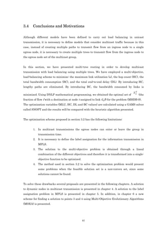
dynamic multicast routings that does not consider QoS.
2.4 Conclusions and Motivations
In this section, we have presented some fundamental concepts and different related works
with this research. The concepts presented in this chapter allow us to put our research into a
context and understand the different related works helping us to make some proposals for
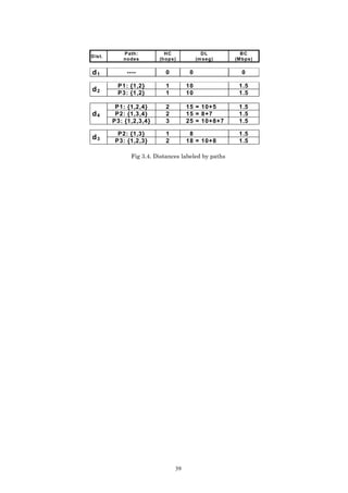
multicast transmissions in chapters 3, 4, 5 and 6.
30](https://image.slidesharecdn.com/programacionmultiobjetivo-121118123824-phpapp02/85/Programacion-multiobjetivo-50-320.jpg)
![Chapter 3 Load Balancing of Static Multicast Flows
3.1 Overview
Although different models have been defined, which fulfill load balancing in unicast
transmission, it is necessary to define other models that consider multicast transmission,
because in this case, instead of creating multiple paths to transmit the flow from the ingress
node to just one egress node it is necessary to create multiple trees to transport the flow from
the ingress node to the egress node set of the multicast group.
In this chapter we propose a load-balancing scheme using several objectives to create multiple
trees based on weighting methods. The scheme includes the maximum link utilization (MLU),
the hop count (HC), the total bandwidth consumption (BC), and the total end-to-end delay
(DL). In this model, we have included a constraint with the aim of solving the scalability
problem, because without this constraint it would be possible to create too many trees.
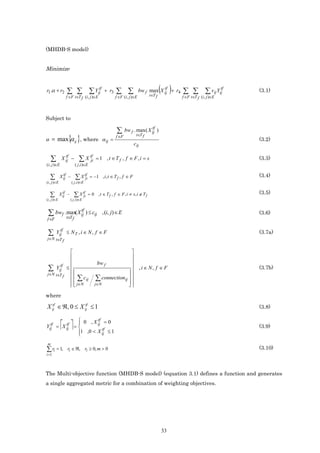
3.2 Optimization Scheme
In this multi-objective proposal the network is modeled as a directed graph G = ( N , E ) , where
N is the set of nodes and E is the set of links. We use n to denote the number of network nodes,
i.e. n = N . Among the nodes, we have a source s ∈ N (ingress node) and some destinations T
(the set of egress nodes). Let t ∈ T be any egress node. Let (i, j ) ∈ E be the link from node i
to node j. Let f ∈ F be any multicast flow, where F is the flow set and T f is the egress node
subset for the multicast flow f. We use |F| to denote the number of flows. Note that
T= UT f .
f ∈F
tf
Let X ij be the fraction of flow f to egress node t assigned to link (i,j). Note that these variables
include egress node t, which is not considered in previous works [KIM02] [LEE02] [ROY02]
[SEO02] [WAN01]. Including the egress nodes permits us to control the bandwidth
consumption in each link with a destination at the set of egress nodes. Therefore, it is possible
to maintain the flow equilibrium constraint at the intermediate nodes exactly. The problem’s
tf
solution, X ij variables, provides optimum flow values.
31](https://image.slidesharecdn.com/programacionmultiobjetivo-121118123824-phpapp02/85/Programacion-multiobjetivo-51-320.jpg)

![The main objective consists in minimizing the maximum link utilization (MLU), which is
represented by α in (3.1). The value of α is directly related to the utilization in each link (i,j).
However with this objective the solution obtained may involve long routes. In order to
eliminate these routes and to minimize hop count (HC), the term ∑ ∑ ∑ Y tf
ij is added.
f ∈F t∈T f ( i , j )∈E
This is necessary because the objective function may report only the most congested link and
the optimal solution may include unnecessarily long paths in order to avoid the bottleneck link
[KIM02].
In addition, in the hop count function it is possibly to optimize other objective functions, for
example, in order to minimize the total bandwidth consumption (BC) over all links, the term
∑ ∑ tf
bw f max X ij
t∈T f
( ) is also added. Remember that in a unicast connection, the total amount
f ∈F t (i , j )∈E
of bandwidth consumed by all the flows with a destination at egress node t must not exceed
the maximum utilization (α) per link capacity cij, that is, ∑ bwf ∑.Xij ≤ cij.α, (i, j) ∈ E . However in a
tf
f ∈F t∈T
multicast connection it is necessary to consider only the maximum value because the same
packet is never sent twice in a link.
Furthermore, in order to minimize the total end-to-end propagation delay (DL) over all links,
the term ∑ ∑ ∑ vij Y tf is also added. In [ABO98] the authors showed that the delay has
ij
f ∈F t∈T f ( i , j )∈E
three basic components: switching delay, queuing delay and propagation delay. The switching
delay is a constant value and can be added to the propagation value. The queuing delay is
already reflected in the bandwidth consumption. The authors state that the queuing delay is
used as an indirect measure of buffer overflow probability (to be minimized). Other
computational studies (e.g. [ABO98]) have shown that it makes little difference whether the
cost function used in routing includes the queuing delay or the much simpler form of link
utilization.
Equation (3.2) calculates the maximum link utilization (MLU), also called α, in function of the
maximum utilization in every link (i,j) in which a fraction of the multicast flow is being
transmitted.
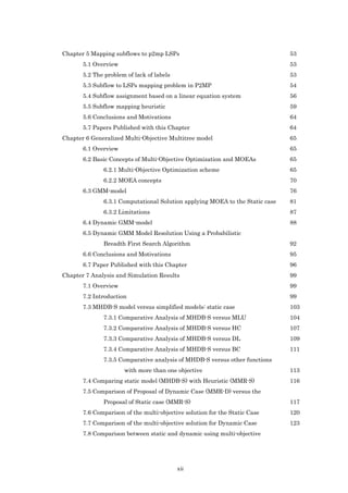
Constraints (3.3), (3.4) and (3.5) are flow conservation constraints. Constraint (3.3) ensures
that the total flow emerging from the ingress node to any egress node t at flow f is 1. In Fig 3.1
34](https://image.slidesharecdn.com/programacionmultiobjetivo-121118123824-phpapp02/85/Programacion-multiobjetivo-54-320.jpg)
![and Fig 3.2 we show that the sum of the X values leaving the ingress node (Node 1) with
destinations at every egress node (Nodes 5 and 6) is 1. In the Figures 3.1 and 3.2 we show an
example of the creation of two trees to transmit one multicast flow. In this example the ingress
node is node 1 and the egress nodes are nodes 5 and 6. In this example using the proposal
presented in this chapter, it is possible to create two trees to transmit the multicast flow. In
this case, the variable X represents the fraction of flow transmitted in every link with a
destination at one particular egress node.
5
X 25 = 0.5 LSP3
LSP1 2 5
X
5
= 0.5 2 5
12
5
X 45 = 0.5
5
LST1
1
LST2
1
X 14 = 0.5
4 4
6
X 14 = 0.5
6
LSP2 6
X 46 = 0.5
X 13 = 0.5 3 6 LSP4
6 3 6
X 36 = 0.5
Fig 3.1. 1st Transmission Tree in Multicast Fig 3.2. 2nd Transmission Tree in Multicast
Constraint (3.4) ensures that the total flow coming from an egress node t at flow f is 1.
Constraint (3.5) ensures that for any intermediate node that is different from the ingress node
(i ≠ s) and egress nodes (i ∉ T ) , the sum of its output flows to egress node t minus the input
flows with a destination at egress node t at flow f is 0. i.e.
(x 5
25
5 6
)( 6 5 5
)( 6 6
− x12 = 0 , x36 − x13 = 0 , x 45 − x14 = 0 , x 46 − x14 = 0 . )( )
Constraint (3.6) is the maximum link utilization constraint. Remember that in an unicast
connection, the total amount of bandwidth consumed by all the flows with a destination at
egress node t must not exceed the maximum utilization (α) per link capacity cij, that is,
∑ bwf ∑.Xij ≤ cij.α, (i, j) ∈ E .
tf
f ∈F t∈T
Nevertheless, in constraint (3.6) only the maximum value of X ij for t ∈ T f must be considered.
tf
Though several subflows of flow f in link (i,j) with destinations at different egress nodes are
sent, in multicast IP specification just one subflow will be sent.
The function max in expressions (3.1), (3.2) and (3.6) generates discontinuous derivatives. For
this reason, the problem should be solved using a GAMS tool to solve DNLPs (Nonlinear
programming with discontinuous derivatives) such as MINOS, MINOS5, COMOPT,
COMOPT2, and SNOPT [GAM04]. The DNLP problem is the same as the NLP (Nonlinear
Programming) problem, except that non-smooth functions (abs, min, max) can appear.
35](https://image.slidesharecdn.com/programacionmultiobjetivo-121118123824-phpapp02/85/Programacion-multiobjetivo-55-320.jpg)
![Our model is a nonlinear programming problem because some equations use the nonlinear
function max (3.1), (3.2), (3.6). Usually the models can be relaxed by introducing a new
constraint variable which reaches the greatest value of the max function. One way to give a
solution to this kind of problem is the linearization. For example: min y, where y = max xi,
such model can be rewritten as: min y, where y ≥ xi. But sometimes, such relaxation can
introduce new variables in the model and this kind of solution (called e-constraint) has
problems when in multi-objective optimization problem the solution space is not convex:
Moreover, another difficult it is to know the maximum values of these new constraints. This
kind of method to convert a nonlinear problem into a linear problem is good when the problem
is a single-objective problem. And this kind of solution is good when it is impossible to have a
nonlinear solver.
The constraints (3.7a) and (3.7b) limit the maximum number of subflows in each node by
means of the capacity of each link and the traffic demand. This formulation represents the
number of links necessary for a traffic demand, without this constraint the model could have
scalability problems, i.e. the label space used by the LSPs would be too high.
A first approach towards achieving this aim is to use constraint (3.7a), in this case, the
maximum number of necessary links is given by a constant value NT [DON03]. However, this
expression has a problem; what is the right value of NT? To solve this drawback constraint
(3.7b), which depends on network characteristics (flow demand, bandwidth in every link and
number of connections in every node), is defined.
tf
Expression (3.8) shows that the X ij variables must be real numbers between 0 and 1 because
they represent the fraction of every flow that is transmitted. These variables form multiple
trees to transport multicast flow. The demand between the ingress node and egress node t can
be split over multiple routes. When the problem is solved without load balancing, this variable
can only take the values 0 and 1, which show, respectively, whether or not link (i,j) is being
used to carry information to egress node t.
tf tf tf
Expression (3.9) calculates Yij as a function of X ij . Note that the variables Yij are integers.
Finally, expression (3.10) shows that the weighting coefficients, ri, assigned to the objectives
are normalized. These values are used to solve the optimization problem.
36](https://image.slidesharecdn.com/programacionmultiobjetivo-121118123824-phpapp02/85/Programacion-multiobjetivo-56-320.jpg)


![3.5 Papers Published with this Chapter
International Journals
• [DON05] Y. Donoso, R. Fabregat, JL. Marzo. “Multicast Routing With Traffic Engineering:
A Multi-Objective Optimization Scheme And A Polynomial Shortest Path Tree Algorithm
With Load Balancing.” Annals of Operations Research. Kluwer Publisher. 2005.
• [DON04c] Y. Donoso, R. Fabregat, JL. Marzo. “Multi-Objective Optimization Algorithm for
Multicast Routing with Traffic Engineering.” Telecommunication Systems Journal. Kluwer
Publisher. 2004.
International Conference
• [FAB04a] R. Fabregat, Y.Donoso, JL. Marzo, A. Ariza. “A Multi-Objective Multipath
Routing Algorithm for Multicast Flows.” International Symposium on Performance
Evaluation of Computer and Telecommunication Systems (SPECTS'04). San Jose, USA.
July 2004.
• [DON04] Y. Donoso, R. Fabregat, JL. Marzo. “Multi-Objective Optimization Algorithm for
Multicast Routing with Traffic Engineering”. IEEE 3rd International Conference on
Networking ICN'04, Guadeloupe, French Caribbean, March 2004. Selected as Best Papers.
• [DON04d] Y. Donoso, R. Fabregat, JL. Marzo. “Multi-Objective Optimization Model and
Heuristic Algorithm for Multipath Routing of Static and Dynamic Multicast Group.” III
Workshop on MPLS Networks. Girona, Spain. March 2004.
• [DON04e] Y. Donoso, R. Fabregat, JL. Marzo. “Multicast Routing with Traffic
Engineering: a Multi-Objective Optimization Scheme and a Polynomial Shortest Path Tree
Algorithm with Load Balancing”. Proceedings of CCIO -2004 Cartagena de Indias,
Colombia, March 2004. Operation Research National Award given by the Colombian
Operations Research Society. March 2004.
• [DON03] Y. Donoso, R. Fabregat. “Multi-Objective Scheme over Multi-Tree Routing in
Multicast MPLS Networks”. IFIP/ACM Latin America Networking Conference 2003
(LANC03), IFIP-TC6 and ACM SIGCOMM, La Paz (Bolivia). October 2003.
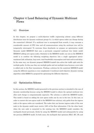
42](https://image.slidesharecdn.com/programacionmultiobjetivo-121118123824-phpapp02/85/Programacion-multiobjetivo-62-320.jpg)
![In the next paper a simplified model for solving the SOP (single-objective problem) for
minimizing α is presented.
• [DON03a] Y. Donoso, R. Fabregat. “Ingeniería de Tráfico aplicada a LSPs Punto-
Multipunto en Redes MPLS”. CLEI (Congreso Latinoamericano de Estudios en
Informática) 2003. La Paz, Bolivia. October 2003.
43](https://image.slidesharecdn.com/programacionmultiobjetivo-121118123824-phpapp02/85/Programacion-multiobjetivo-63-320.jpg)


![transmitted through each one. With regards to limitation 4 in the GMM-model, 11 objective
functions for optimization have been included.
4.5 Papers Published with this Chapter
International Conference
• [DON04a] Y. Donoso, R. Fabregat, JL. Marzo. “Multi-Objective Optimization Model and
Heuristic Algorithm for Dynamic Multicast Routing”. IEEE & VDE Networks 2004.
Vienna, Austria. June 2004.
• [DON04b] Y. Donoso, R. Fabregat, JL. Marzo. “Multi-Objective Optimization Scheme for
Dynamic Multicast Groups”. IEEE ISCC (The 9th IEEE Symposium on Computers and
Communications). Alexandria, Egypt. June 2004.
• [DON04e] Y. Donoso, R. Fabregat, JL. Marzo. “Multi-Objective Optimization Model and
Heuristic Algorithm for Multipath Routing of Static and Dynamic Multicast Group”. III
Workshop on MPLS Networks. Girona, Spain. March 2004.
52](https://image.slidesharecdn.com/programacionmultiobjetivo-121118123824-phpapp02/85/Programacion-multiobjetivo-72-320.jpg)
![Chapter 5 Mapping subflows to P2MP LSPs
5.1 Overview
In this chapter we focus on the specific problem of mapping subflows to point-to-multipoint
(P2MP) LSPs for MPLS network implementations. The aim is to obtain an efficient solution to
formulate P2MP LSPs given a set of optimum subflow values. In [SOL04] the author presents
a subflow mapping solution based on a linear equation system that requires a large number of
equations and variables. To solve this problem, a subflow mapping heuristic for creating
multiple P2MP LSPs based on the optimum subflow values obtained with the MHDB-S model
is proposed in this sub-section.
5.2 The problem of lack of labels
A general problem of supporting multicasting in MPLS networks is the lack of labels. The
MPLS architecture allows aggregation in point-to-point (P2P) LSPs. Aggregation reduces the
number of labels that are needed to handle a particular set of flows, and may also reduce the
amount of label distribution control traffic needed [ROS01]. Adding new LSPs increases the
label space and hence the lookup delay. Therefore, reducing the number of labels used is a
desirable characteristic for any algorithm that maps flows to LSPs.
As pointed out in [ROS01], the label based forwarding mechanism of MPLS can also be used to
route along multi-point to point (MP2P) LSPs. In [SAI00] and [BHA02], aggregation
algorithms that merge P2P LSPs into a minimal number of MP2P LSPs are considered. In this
case, labels assigned to different incoming links are merged into one label assigned to an
outgoing link. If two P2P LSPs follow the same path from an intermediate node to the egress
node, these aggregation algorithms allocate the same label to the two P2P LSPs and thus
reduce the number of labels used. In [APP03], an algorithm that reduces the number of MPLS
labels for |N| (number of nodes) + |E| (number of links) without increasing the link load is
presented. For differentiated services with K traffic classes with different load constraints,
their limit increases to K(|N|+|E|). Their stack-depth is only one, justifying MPLS
implementations with limited stack depths. To reduce the number of labels used for multicast
traffic, another label aggregation algorithm is presented in [OH03]. In this case, if two P2MP
53](https://image.slidesharecdn.com/programacionmultiobjetivo-121118123824-phpapp02/85/Programacion-multiobjetivo-73-320.jpg)
![LSPs follow the same tree from an ingress node to the egress node set, the aggregation
algorithm allocates the same labels to the two P2MP LSPs. Ingress nodes have a new table
(called the Tree Node Table), which saves node information from the P2MP LSP. Label
allocation is carried out using this table.
The label stack was introduced into the MPLS framework to allow multiple LSPs to be added
to a single LSP tunnel [ROS01]. In [GUP03], a comprehensive study of label size versus stack
depth trade-off for MPLS routing protocols in lines and trees is undertaken. This study shows
that, in addition to LSP tunneling, label stacks can also be used to dramatically reduce the
number of labels required to set up LSPs in a network. Their protocols have numerous
practical applications that include implementing multicast trees, and virtual private networks
using MPLS as the underlying signaling mechanism.
5.3 Subflow to LSPs mapping problem in P2MP
In this section, we detail the problem of mapping multiple P2MP LSPs based on the optimum
tf
subflow values X ij obtained with the MHDB-S model (3.1). However, this mapping is difficult
using the MHDB-S model because there is no index for identifying subflows [SOL04].
tf
Remember that X ij is the fraction of flow f with a destination at node t assigned to link (i,j). As
the presented algorithm applies only to one flow f, the index f will be omitted when it does not
cause confusion.
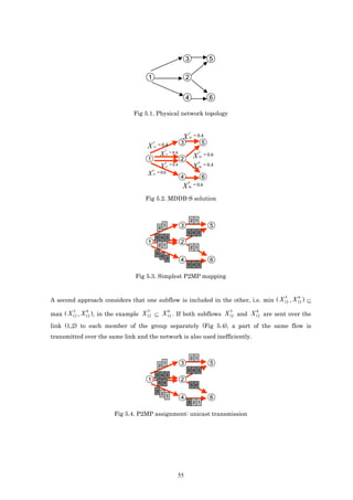
To explain the problem, the MHDB-S models have been applied to the topology of Fig 5.1, with
t
a single flow f, where s=N1 and T={N5, N6}. In this case, a possible subflow solution ( X ij )
obtained is shown in Fig. 5.2. The simplest solution (Fig. 5.3.) to create LSPs based on the
optimum subflow values is to send each subflow (0.4 and 0.6 fractions) to the group separately,
and in this case each subflow is mapped to one P2MP LPS. In Fig. 5.3, each packet represents
5 6
a 0.2 fraction of the flow. With this mapping, subflows X 12 and X 12 are different and the
maximum link utilization constraint (5) could be violated. Moreover, the network is used
inefficiently because multicast node capabilities are not considered. In section 3.2 the
difference between the multicast and unicast equations in the bandwidth consumption
constraint was explained.
54](https://image.slidesharecdn.com/programacionmultiobjetivo-121118123824-phpapp02/85/Programacion-multiobjetivo-74-320.jpg)


![5.6 Conclusions and Motivations
In this chapter, we have presented a proposal for finding a solution for label assignation and
the creation of LSPs in MPLS technology. With this proposal, we have given a solution for
limitation 2 presented at the end of chapter 4.
However, we still have the other limitations: solving the multi-objective problem is given
through lineal combination and this model does not cover some objective functions analyzed by
other authors.
In the next chapter we propose a generalized model with 11 different objective functions and
the solution is given in a real multi-objective context using MOEAs (Multi-Objective
Evolutionary Algorithms).
5.7 Papers Published with this Chapter
International Conference
• [SOL05] F. Solano, R. Fabregat, Y. Donoso, JL. Marzo. “Asymmetric Tunnels in P2MP
LSPs as a Label Space Reduction Method”. IEEE ICC 2005. Seoul, Korea. May 2005.
• [SOL04a] F. Solano, R. Fabregat, Y. Donoso, JL. Marzo. “Mapping subflows to P2MP
LSPs”. IEEE International Workshop on IP Operations & Management (IPOM 2004).
Beijing, China. October 2004.
• [SOL04] F. Solano, R. Fabregat, Y. Donoso. “Subflow assignment model of multicast
flows using multiple P2MP LSPs”. CLEI (Congreso Latinoamericano de Estudios en
Informática) 2004. Arequipa, Perú. October 2004.
64](https://image.slidesharecdn.com/programacionmultiobjetivo-121118123824-phpapp02/85/Programacion-multiobjetivo-84-320.jpg)
![Chapter 6 Generalized Multi-Objective Multitree
model
6.1 Overview
In the previous chapters we presented the proposal for solving the multi-objective problem
using load balancing in multicast transmissions. In the last chapters the problem was solved
using the weighted sum method. In addition, the limitations and problems of the proposals
were presented:
• The solutions found using the weighted sum method present problems when the space
of feasible solutions is not convex. Since this method works with linear combinations,
it is possible that many solutions cannot be found.
• In the dynamic case the solution found is sub-optimal.
• Only some objectives of those presented in other related works have been considered.
To overcome these drawbacks, in this chapter we propose a Generalized Multiobjective
Multitree model (GMM-model) in a pure multiobjective context that considers simultaneously
for the first time multicast flow, multitree, and splitting. A Multiobjective Evolutionary
Algorithm (MOEA) approach is proposed to solve the GMM-model.
6.2 Basic Concepts of Multi-Objective Optimization and MOEAs
6.2.1 Multi-Objective Optimization scheme
A general MOP includes a set of n parameters (decision variables), a set of k objective
functions and a set of m restrictions. The objective and restriction functions are functions of
the decision variables [COL03] [COH78]. Then the MOP can be expressed as:
65](https://image.slidesharecdn.com/programacionmultiobjetivo-121118123824-phpapp02/85/Programacion-multiobjetivo-85-320.jpg)


![Definition 6.5: Pareto Optimality. Given a decision vector x ∈ Xf and its corresponding
objective vector y = f(x) ∈ Yf , it is said that x is not dominated with respect to a set A ⊆ Xf if
and only if
∀ a ∈ A : (x ≻ a ∨ x ∼ a) (6.7)
In case x is not dominated with respect to the entire set Xf, and only in that case, it is said that
x is a Pareto optimal solution (x ∈ Xtrue, the real Pareto’s optimal set). While the
corresponding y is part of the real Pareto optimal front Ytrue. This is defined as follows.
Definition 6.6: Pareto optimal set and Pareto optimal front. Given the set of feasible decision
vectors Xf. Xtrue will be the set of non-dominated decision factors belonging to Xf. That is:
Xtrue = { x ∈ Xf | x is not dominated with respect to Xf } (6.8)
The set Xtrue is also known as the Pareto optimal set. While the corresponding set of objective
vectors Ytrue = f(Xtrue) constitutes the Pareto optimal front.
Now, the MOP involves two conceptually distinct tasks: search and decision making [HOR97].
Search is related to the processes where the feasible solutions are visited in order to find the
Pareto optimal solutions. Decision making refers to the ranking process of alternative
solutions. A rational human decision maker determines preferences among the conflicting
objectives. The methodologies in MOP can be classified into three primary groups, depending
on how the search and decision making tasks are handled. Horn [HOR97] discusses the state-
of-art approaches for each of these methodologies in detail [CER04]:
• Decision making before search: In this approach, the objectives are aggregated into
a single objective function where the preference information of the decision maker
is represented. The aggregation can be carried out in two ways: scalar combination
or lexicographical ordering (ranking according to the importance) of the objectives.
The aggregation of the objectives into a single objective function requires domain-
specific knowledge about the ranges and the behavior of the functions. However,
this kind of deep knowledge about the functions is usually not available, since the
functions and/or feasible set may be too complex. However, this methodology has
the advantage that the SOP strategies can be applied to the problem with the
aggregated objective.
69](https://image.slidesharecdn.com/programacionmultiobjetivo-121118123824-phpapp02/85/Programacion-multiobjetivo-89-320.jpg)
![• Search before decision making: The feasible set is searched to find a set of best
alternatives, without giving any information about preferences. Decision making
considers only the reduced set of alternatives. For most of the real-life problems,
gaining fundamental knowledge about the problem and alternative solutions can
be very helpful in realizing the conflicts that are inherent in the problem.
Performing the search before decision making makes this favorable circumstances
possible, however the search process becomes more difficult with the exclusion of
the preferences of the decision maker.
• Integrating search and decision making: This approach includes the interactive
methods where the preferences of the decision maker are used during the search
process. At each iteration, the result of the search is evaluated by the decision
maker in order to update the preferences. The search space is then reduced and the
direction of the search is restricted to some particular regions according to the
preferences of the decision maker. This last methodology integrates the theory of
decision making into optimization theory.
The interest of this thesis is in the first and in the second categories and comparisons between
these kinds of methodologies are shown in the chapter 7. The first categories are given by the
proposals presented in the chapters 3 and 4. The second category is given by the proposal
presented in this chapter. In the second category when the method obtain an optimal solution
set a rational human decision maker determines preferences among the conflicting objectives.
6.2.2 MOEA concepts
The term evolutionary algorithm (EA) refers to searching and optimization techniques
inspired by the evolution model proposed by Charles Darwin after his exploratory trips
[BAC00].
In nature individuals are characterized by chains of genetic material that are denominated by
chromosomes. All information related to the individual and his or her tendencies is coded in
the chromosomes. Each element making up the chromosome is called an allele. Each
individual has an adaptation level to the environment, which gives him or her a greater
survival capacity and possibility to generate descendants. This level of adaptation is linked to
the characteristics encoded in the chromosomes. As the genetic material can be passed from
parents to children as pairing occurs, the resulting children have chromosome chains
resembling those of their parents and they combine characteristics of both. So, if two parents
70](https://image.slidesharecdn.com/programacionmultiobjetivo-121118123824-phpapp02/85/Programacion-multiobjetivo-90-320.jpg)
![with good characteristics cross, they will probably generate equally good children or even
better ones [DEB01].
In order to solve a searching or optimization problem using evolutionary algorithms and the
suggested concepts first a given number of possible solutions to the problem are presented as
individuals of a finite population. This process is called coding. When coding an individual, all
the relevant information concerning the individual and considered to influence optimization or
searching must be present. Generally, the coding of an individual or its chromosome is a chain
of bits or round numbers, depending on the problem to be solved. In this chain the element
located in a given position is called an allele.
Next the ability or adaptation level of each individual is determined (fitness), depending on the
quality of the solution it represents. Later, the existing individuals generate new individuals
through genetic operators such as selection, crossing or mutation. The selection operator
chooses the parents that will be crossed. The probability that an individual is chosen as a
parent and/or that it survives up to the next generation is linked to its fitness or ability; the
greater the fitness, the greater the probability of surviving and having descendants, in the
same way that it occurs in natural processes.
After choosing the parents, their recombination or crossing occurs in order to obtain a new
generation. In this way, in every new generation there is a high probability that the new
population is composed of better individuals, since the offspring inherit the good
characteristics of their parents, which when combined will be better.
On the other hand, during recombination alterations (mutations) may occur in an individual’s
genetic information. If the alterations that occur are good, they will generate a good individual
with a high fitness and the alteration will be transmitted to the next generation; if, on the
contrary, the alteration is not beneficial, the altered individual will have a low fitness and very
few descendants or none at all. If this is so, this alteration will disappear with it. In this way,
after several generations, the population will have evolved genetically to be individuals with a
high ability level. That is to say, they represent good solutions to the proposed problem.
The operators described are called searching or genetic operators. Reproduction focuses its
attention on individuals with a high degree of fitness, and in this way, it takes advantage of
the information at hand concerning the adaptation of the individual to the environment.
Recombination and mutation somehow disturb individuals and they provide heuristics for the
exploration of searching spaces. This is why the Eas are said to use the concepts of exploitation
71](https://image.slidesharecdn.com/programacionmultiobjetivo-121118123824-phpapp02/85/Programacion-multiobjetivo-91-320.jpg)
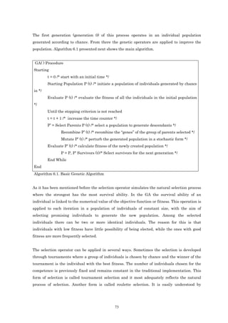
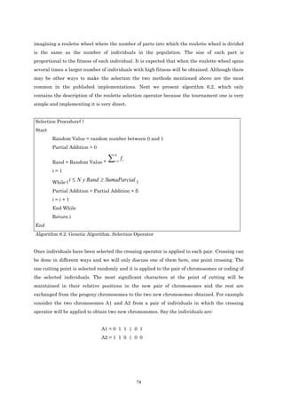
![Where the “|” symbol indicates the cut point. The characters on the left of the cutting point
are the most significant, so they remain in their corresponding positions in the new
chromosomes, while the characters to the right of the cutting point are crossed with the
parental chromosomes as shown in the example:
A’1 = 0 1 1 | 0 0
A’2 = 1 1 0 | 0 1
In this way A’1 and A’2 are the chromosomes resulting from applying the crossing operator to
the pair of parental chromosomes
In Algorithm 6.3 the crossing operator is described. In the already mentioned pseudo-code I
represents the length (in bits) of the chromosome; Jcross is the cutting point; the vectors
Descendant 1 and Descendant 2 are equivalent to the binary representation of a pair of
descendants; and Parent 1 and Parent 2 are the parents. The given crossing probability
indicates the probability that parents will cross and the probability of generating clones. In
this way not all selected individuals are destroyed by crossing.
CrossOver Procedure(Parent1, Parent2)
Start
Rand = random number between 0 and 1
If Rand is Lower than the given crossing probability
JCross = random number between 1 and l
If not
JCross = l
End Si
From i = 1 to i = JCross, i = i + 1
Offspring1[i] = Parent1[i]
Offspring2[i] = Parent2[i]
End From
From i = Jcross + 1 to i = l, i = i + 1
Offspring 1[i] = Parent2[i]
Offspring2[i] = Parent1[i]
End From
End
Algorithm 6.3. Genetic Algorithm. Crossover Operator
75](https://image.slidesharecdn.com/programacionmultiobjetivo-121118123824-phpapp02/85/Programacion-multiobjetivo-95-320.jpg)
![The crossing operator represents a form of local search in the regions next to the searching
space surrounding the parents. On the other hand the mutation process is basically an random
search. A specific position in the chromosome of the mutating individual is selected in an
random way, then, the content value in that position is changed.
In nature the probability of a mutation occurring is small in normal living conditions. In the
GA we try to represent the same probability with a very low occurrence value for the mutation
operator.
Evolutionary algorithms and multi-objective optimization
The Eas are interesting given the fact that at first glance they seem especially apt to deal with
the difficulties presented by MOPs. The reason for this is that they can return an entire set of
solutions after a simple run and they do not have any other of the limitations of traditional
techniques. In addition, some researchers have suggested that the Eas would behave better
than other blind searching techniques. This statement still needs a clear demonstration and it
should be considered in the light of the “no free lunch” theorems related with optimization,
which states that if a method behaves “better” than other methods in one set of problems, it
will perform “worse” in another set. The reality is that nowadays there are very few valid
alternatives concerning other possible solution methods. In fact, the most recent publications
on MOP resolutions using Eas (which are compiled in [DEB01]), seem to consider this fact and
they have opened the way to a whole new field of research: evolutionary algorithms applied to
multi-objective optimization (MOEA): Multiobjective Optimization Evolutionary Algorithm).
6.3 GMM-model
The proposed GMM-model considers a network represented as a graph G(N, E), with N
denoting the set of nodes and E the set of links. The cardinality of a set is denoted as |.|, thus
|N| represents the cardinality of N.
The set of flows is denoted as F. Each flow f ∈ F can be split into Kf subflows that after
normalization can be denoted as fk; k = 1, … |Kf|. In this case, fk indicates the fraction of f ∈ F
it transports, i.e.
Kf (6.9)
∑f
k =1
k =1
76](https://image.slidesharecdn.com/programacionmultiobjetivo-121118123824-phpapp02/85/Programacion-multiobjetivo-96-320.jpg)
![For each flow f ∈ F we have a source sf ∈ N and a set of destination or egress nodes Tf ⊂ N.
Let t be an egress node, i.e. t ∈Tf.
f t
Let X ij k denote the fraction of subflow fk to egress node t assigned to link (i,j) ∈ E, i.e.
f t f t
0≤ X ij k ≤1. In this way, the n components of decision vector X are given by all X ij k . Note that
X ijf k t uses five indexes: i, j, f, k and t for the first time, unlike previous publications that only
used a smaller subset of indexes because they did not deal with the same general problem
[KIM02] [LEE02] [ROY02] [SEO02] [WAN01]. In particular, the novel introduction of a
subflow index k gives an easy way to identify subflows and define LSPs in a MPLS
implementation.
Let cij be the capacity (in bps) of each link (i,j) ∈ E. Let bf be the traffic request (measured in
bps) of flow f ∈ F, traveling from source sf to Tf. Let dij be the delay (in ms) of each link (i,j) ∈
f t
E. The binary variables Yij k represent whether a link (i,j) is being used (value 1) or not (value
0) for transporting subflow fk to destination node t, i.e.
0, if X ijf k t = 0
Yijf k t = X ijf k t = (6.10)
1, otherwise
where
. denotes the ceiling function and consequently, . denotes the floor function.
Finally, let connectionij be an indicator of whether there is a link between nodes i and j.
Given the above notation and the multiobjective context already presented in equation (6.1),
the proposed GMM-model considers the following objective functions:
Maximal link utilization
F Kf
φ1 = max α ij { } where α ij =
1
cij
∑∑ b f { }
max X ijf k t (6.11)
f =1 k =1 t ∈T f
Hop count, in several different flavors such as:
Total hop count
φ2 = ∑ ∑ ∑ ∑Y
( )
i , j ∈E f ∈F k ∈K f t∈T f
ij
fkt
(6.12)
Hop count average
77](https://image.slidesharecdn.com/programacionmultiobjetivo-121118123824-phpapp02/85/Programacion-multiobjetivo-97-320.jpg)


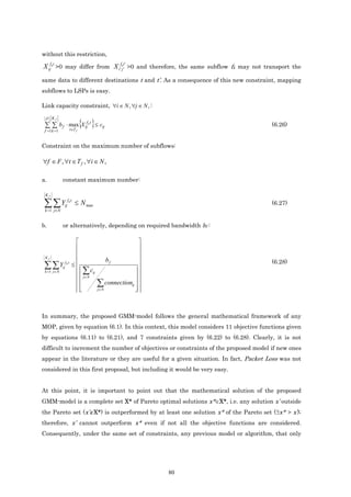
![considers a subset of the proposed objective functions, either as a SOP or MOP, can find one or
more solutions calculated with the GMM-model or dominated by solutions x*∈X* of this model.
In conclusion, by using the GMM-model it is possible to calculate the whole set of optimal
Pareto solutions. This includes any solution that has been found previously using most of the
already published alternatives that consider any subset of the proposed objective functions.
Now it is clear why we call this model generalized.
6.3.1 Computational Solution applying MOEA to the Static case
To solve the GMM-model, a Multiobjective Evolutionary Algorithm (MOEA) approach has been
selected because of its well recognized advantages when solving MOPs in general and TE load
balancing in particular [CRI04], [CRI04a], [CRI04b], [FAB04], [KOY04], [ROY02], [CUI03] and
[ROY04]. A MOEA, as a genetic algorithm, has been inspired by the mechanics of natural
evolution (based on the survival of the fittest) [VAN99].
At the beginning, an initial population of Pmax feasible solutions (known as individuals) is
created as a starting point for the search. In the next stages (or generations), a performance
metric, known as fitness, is calculated for each individual. In general, a modern MOEA
calculates fitness considering the dominance properties of a solution with respect to a
population. Based on this fitness, a selection mechanism chooses good solutions (known as
parents) for generating a new population of candidate solutions, using genetic operators like
crossover and mutation [GOL89]. The process continues iteratively, replacing old populations
with new ones, saving the best found solutions (a process known as elitism), until a stop
condition is reached.
In this chapter, an algorithm based on the Strength Pareto Evolutionary Algorithm (SPEA)
[ZIT99] is proposed. It has an evolutionary population P and an external set Pnd with the best
Pareto solutions found. Starting with a random population P, the individuals of P evolve to
optimal solutions that are included in Pnd. Old dominated solutions of Pnd are pruned each time
a new solution from P enters Pnd and dominates old ones.
Encoding
Encoding is the process of mapping a decision variable x into a chromosome (the
computational representation of a candidate solution). This is one of the most important steps
towards solving a TE load balancing problem using evolutionary algorithms. Fortunately, it
has been studied a lot in current literature. However, it should be mentioned that to our best
81](https://image.slidesharecdn.com/programacionmultiobjetivo-121118123824-phpapp02/85/Programacion-multiobjetivo-101-320.jpg)

![• A first subflow (k=1) transmits 40% of the total flow information through (Tree f,1)
which consists of two different paths, (Path f,1,5)={N1, N2, N5} and (Path f,1,6)={N1, N2,
N6}.
• A second subflow (k=2) transmits 20% of the total flow through (Tree f,2) using two
different paths, (Path f,2,5)={N1, N2, N5} and (Path f,2,6)={N1, N4, N6}.
• Finally, a third subflow (k=3) transmits the final 40% of the total flow through (Tree
f,3), which consist of two different paths, (Path f,3,5)={N1, N3, N5} and (Path f,3,6)={N1,
N4, N6}.
(Subflow f,1) (Subflow f,2) (Subflow f,2)
N3 N3 N3
N5 N5 N5
N2 N2 N2
N1 N1 N1
N4 N4 N4
N6 N6 N6
ff1=0.4 ff2=0.2 ff3=0.4
sf={N1} Tf ={N5 , N6}
[
(Flow f = /* Generic flow f split into 3 subflows
(Subflow f,1 = ( /* first subflow
Tree f,1=(
Path f,1,5 = (N1,N2,N5), /* path to destination N5
Path f,1,6 = (N1,N2,N6) ) ), /* path to destination N6
fraction f1 = 0.4 ) /* subflow 1 transmits 40% of flow
(Subflow f,2 = ( /* second subflow
Tree f,2=(
Path f,2,5 = (N1,N2,N5), /* path to destination N5
Path f,2,6 = (N1,N4,N6) ) ), /* path to destination N6
fraction f2 = 0.2 ) /* subflow 2 transmits 20% of flow
(Subflow f,3 = ( /* third subflow
Tree f,3)=(
Path f,3,5 = (N1,N3,N5), /* path to destination N5
Path f,3,6 = (N1,N4,N6) ) ), /* path to destination N6
fraction f3 = 0.4 ) /* subflow 3 transmits 40% of flow
)
]
Fig 6.3. Network topology and chromosome representation for a flow f with three subflows
83](https://image.slidesharecdn.com/programacionmultiobjetivo-121118123824-phpapp02/85/Programacion-multiobjetivo-103-320.jpg)
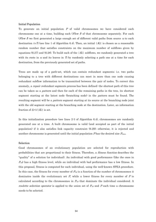
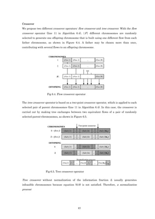

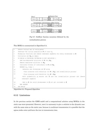


![The complexity of the algorithm is given by the first step. The Breadth First Search
probabilistic function has the next complexity O(nlogn). Every loop has an n as the maximum
number of iterations. Finally, the complexity of the algorithm is O(n3logn).
6.6 Conclusions and Motivations
Given that one of the main contributions of this chapter is to formalize the GMM-model as a
general model, it is interesting to compare it to another recently published model, like the
MHDB-model. When comparing them, we can mention the following advantages of the GMM-
model over the previous MHDB-model:
• The MHDB-model recognizes the multiobjective nature of the load balancing problem
considering four objective functions (φ1, φ2, φ6, φ10), but it only solves a SOP using a
weighted sum cost function, therefore only finding one solution for the whole Pareto
set.
• The MHDB-model simultaneously considers a weighted sum of objectives that are
highly correlated, like φ2 and φ6, which seems inefficient in a SOP context. On the other
hand, the GMM-model can also consider correlated objective functions, but only to
discriminate similar solutions in a multi-objective context.
• The weighted sum method proposed in the MHDB-model and several other papers (see
Table II), is not good enough for finding all the solutions of a Pareto set in
multiobjective non-convex problems, as stated in [VAN99].
• Given that the GMM-model clearly identifies each subflow (and even each subpath), it
is very easy mapping subflows to LSPs for MPLS implementations. However, this
mapping is difficult using the MHDB-model because there is no index for identifying
subflows [SOL04].
• Given that each subflow is identified clearly, it is easier and more efficient to extend
this generalized model to the dynamical case given that a node that wants to be
included in a flow only needs to find the “closer” nodes from which subflows can be
obtained.
In this chapter we have proposed a Generalized Multiobjective Multitree model (GMM-model)
that is able to consider any type of flow (unicast and multicast traffic), any number of flows
95](https://image.slidesharecdn.com/programacionmultiobjetivo-121118123824-phpapp02/85/Programacion-multiobjetivo-115-320.jpg)
![(unipath / multipath - unitree / multitree), considering (or not) splitting (or subflows) in a more
general multiobjective context.
If eventually a single-objective context is preferred, techniques like weighted sum may be used
to combine objective functions in a unique cost function that can be combined with restrictions
on some objectives, such as an upper bound on the delay, hop count, etc. However, any optimal
single objective solution, like the ones proposed in several previous papers, could be a solution
of the GMM-model or be dominated by one of its Pareto solutions when all analyzed objective
functions are simultaneously considered.
To solve the proposed model, a Multi-Objective Evolutionary Algorithm (MOEA) inspired by
the Strength Pareto Evolutionary Algorithm (SPEA) has been implemented, proposing a new
encoding process to represent multitree-multicast solutions using splitting.
Finally, we have proposed a dynamic-GMM-model to give a solution to multicast transmission
when the egress nodes can enter and leave in transmission time. A computational solution has
been presented using a Probabilistic Breadth First Search Algorithm. In this case, this
proposal is better than the proposal presented in chapter 4, because in this new proposal we
resolve the dynamic case using every node of the transmission trees, and the computational
solution is given in a real multi-objective context.
6.7 Paper Published with this Chapter
International Conference
• [DON05a] Y. Donoso, R. Fabregat, F. Solano, JL. Marzo, B. Baran. “Generalized
Multiobjective Multitree model for Dynamic Multicast Groups”. IEEE ICC. Seoul. Korea.
May 2005.
• [FAB04] R. Fabregat, Y. Donoso, F. Solano, JL. Marzo. “Multitree Routing for Multicast
Flows: A Genetic Algorithm Approach”. Setè Congrés Català d’Intel·ligència Artificial
(CCIA’2004), Universitat Autònoma de Barcelona, Barcelona (Spain). October 2004.
96](https://image.slidesharecdn.com/programacionmultiobjetivo-121118123824-phpapp02/85/Programacion-multiobjetivo-116-320.jpg)
![Research Reports
• [BAR04] B. Barán, R. Fabregat, Y. Donoso, F. Solano, JL. Marzo. “Generalized
Multiobjective Multitree model”. Proceedings of IIiA Research Report, ref. IIiA 04-08-RR,
Institut d'Informàtica i Aplicacions, University of Girona. September 2004.
97](https://image.slidesharecdn.com/programacionmultiobjetivo-121118123824-phpapp02/85/Programacion-multiobjetivo-117-320.jpg)

![Chapter 7 Analysis and Simulation Results
7.1 Overview
This chapter shows the experiments that have been carried out in order to evaluate the
different models and algorithms proposed (MHDB-S, MMR-S, MHDB-D, MMR-D, GMM-model
and Dynamic GMM-model). These experiments are focussed on testing the different models
and the algorithms in them, as well as taking into account other proposals. First the different
models (mono-objective models and the MHDB-S model) in the static case are tested, and then
the MHDB-S model is compared with the MMR-S algorithms. The results obtained with the
MMR-S algorithm and the MMR-D algorithm are compared. Finally, the results obtained of
the GMM-model through the MOEA solution and the Dynamic GMM-model through BFS
Probabilistic are compared.
The experiments were developed following the methodologies proposed by [MON04] and
[HER03]. These proposals define 7 steps to develop the research evaluation process:
identifying and stating the problem; selecting the factors, levels and ranks; selecting response
variables; choosing the experimental design; developing the experiment; a data statistical
analysis, and finally conclusions and recommendations.
7.2 Introduction
To analyse the performance in extended networks four network scenarios were considered:
NSF (National Science Foundation), SPRINT Network, UUNET Network and several random
networks. These topologies were mainly selected because they have been used in many
previous works.
The NSF network considered has 14 nodes (Fig. 7.1). The costs on the links represent the
delay and all links have 1.5 Mbps of bandwidth capacity.
99](https://image.slidesharecdn.com/programacionmultiobjetivo-121118123824-phpapp02/85/Programacion-multiobjetivo-119-320.jpg)
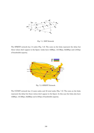
![Fig. 7.3. UUNET Network
Random topologies have been used following the scheme proposed by [MED01]. These
topologies are considered to prove the validity of the MMR-S and MMR-D algorithms proposed
in this thesis in larger topologies than those presented in the three preceding scenarios. Using
this generator several types of net topologies can be obtained by following the traditional
scheme of Internet interconnectivity. It is also possible to obtain other types of topologies using
this generator.
In short, the parameter values used in the tests were the following:
• Transmission rates ranging from 8% of the link capacity to 200%. Exactly 8%,
16%, 33%, 66%, 100%, 133%, 166% and 200%. In this case the flow demand
increases but the number of flows doesn’t.
• The selection of the ingress node was randomly generated.
• The selection of the egress nodes was randomly generated.
• The amount of egress nodes compared with the number of nodes in the network
topology for each flow changed from 20% to 95%. We did not work with 100%
because the ingress node or multicast flow transmitter was not the ingress
node or egress node at the same time.
• Each simulation was developed with one ingress node, which was randomly
selected. The number of egress nodes started at three nodes and in the case of
101](https://image.slidesharecdn.com/programacionmultiobjetivo-121118123824-phpapp02/85/Programacion-multiobjetivo-121-320.jpg)
![• This indicates that adding up GAMS, heuristics and MOEA and probabilistic
BFS 1736 tests were developed in order to establish the corresponding
comparisons.
7.3 MHDB-S model versus simplified models: static case
In this section, the MHDB-S model proposed in chapter 3, which considers four objective
functions, is compared with “traditional” multicast routing algorithms such as DVMRP, PIM-
DM and BGMP, which are mono-objective. In particular, the MHDB-S model is compared with
simple models which only consider one objective function: maximum link utilization in the
MLU-model (section 7.3.1), delay in the DL-model (section 7.3.2), bandwidth consumption in
the BC-model (section 7.3.3) and hop count in the HC-model (section 7.3.4). These models are
proposed in several works: MLU-model in [FOR02], [LEE02] and [ABR02]; DL-model in
[VUT00] and [CHE01]; BC-model in [CHO03] and one cost function which encompasses many
objectives in [LEU98], [INA99], [LI99] and [SUN99].
In section 7.3.5. model MHDB-S is compared with other models, which have more than one
objective and have been presented in other research works. Firstly model MHDB-S is
compared with model DL-BC, considered in [RAO98] and [BAN01], in which only delay and
bandwidth consumption are minimized. Later, model MHDB-S is compared with model HC-BC
considered in [SON03], in which only hop count and bandwidth consumption are minimized.
Finally model MHDB-S is compared with model MLU-HC-DL considered in [ABO98], in which
maximum link utilization, hop count and bandwidth are minimized.
To analyse the analytical model GAMS was used as an optimisation problem solving tool. The
testing consisted in using GAMS to numerically solve the MHDB-S model with the four
objective functions as well as simplified models with only one objective function, which have
been considered in other works ([FOR02], [LEE02], [ABR02] [VUT00], [CHE01], [CHO03],
[LEU98], [INA99], [LI99] and [SUN99]), and also with the models that consider combinations
of two or three objective functions ([RAO98], [BAN01], [SON03] and [ABO98]).
In the following sections the results for NSF are presented. For the SPRINT and UUNET
topologies the same behaviour was observed.
103](https://image.slidesharecdn.com/programacionmultiobjetivo-121118123824-phpapp02/85/Programacion-multiobjetivo-123-320.jpg)
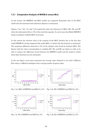
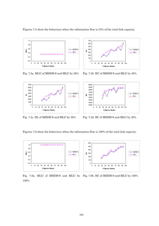

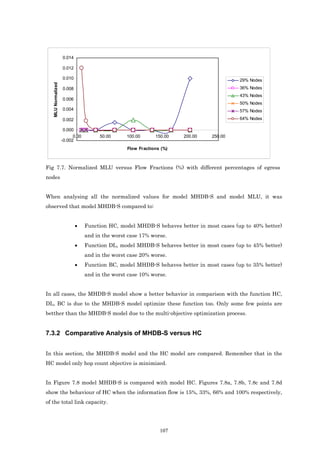
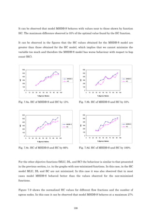
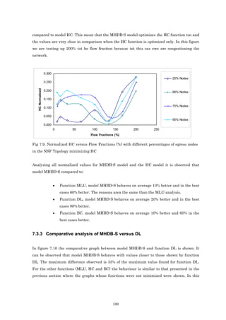
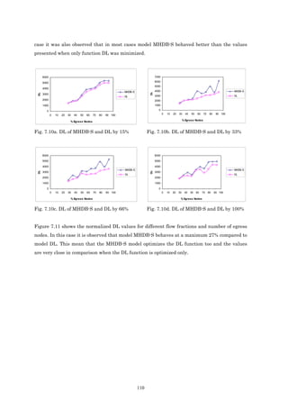
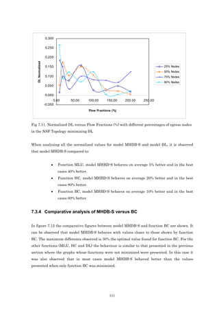
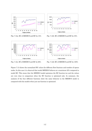
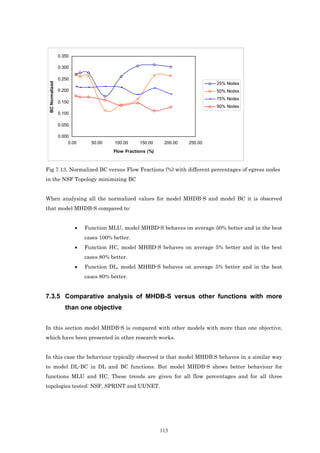
![1.0 800
700
0.8
600
0.6 500 MHDB-S
MHDB-S
MLU
HC
400 DL-BC
0.4 DL-BC
300
200
0.2
100
0.0 0
0 10 20 30 40 50 60 70 80 90 100 0 10 20 30 40 50 60 70 80 90 100
% Egress Nodes % Egress Nodes
Fig. 7.14a. MHDB-S vs DL-BC comparing Fig. 7.14b. MHDB-S vs DL-BC comparing HC
MLU
6000 6000
5000 5000
4000 4000
MHDB-S MHDB-S
DL
3000
BC
3000
DL-BC DL-BC
2000 2000
1000 1000
0 0
0 10 20 30 40 50 60 70 80 90 100 0 10 20 30 40 50 60 70 80 90 100
% Egress Nodes % Egress Nodes
Fig. 7.14c. MHDB-S vs DL-BC comparing DL Fig. 7.14d. MHDB-S vs DL-BC comparing BC
Secondly, model MHDB was compared with model HC-BC [SON03] in which only hop count
(HC) and Bandwidth consumption (BC) are minimized.
In this case the behaviour typically observed is that model MHDB-S behaves in a similar way
to model HC-BC in functions HC and BC. But model MHDB-S shows better behaviour for
functions MLU and DL. These trends are given for all flow percentages and for the three
typologies tested: NSF, SPRINT and UUNET.
1.0 600
0.8 500
400 MHDB-S
0.6 MHDB-S
MLU
HC
300 HC-BC
0.4 DL-BC
200
0.2
100
0.0 0
0 10 20 30 40 50 60 70 80 90 100 0 10 20 30 40 50 60 70 80 90 100
% Egress Nodes % Egress Nodes
Fig. 7.15a. MHDB-S vs HC-BC comparing MLU Fig. 7.15b. MHDB-S vs HC-BC comparing
HC
114](https://image.slidesharecdn.com/programacionmultiobjetivo-121118123824-phpapp02/85/Programacion-multiobjetivo-134-320.jpg)
![8000 60000
7000
50000
6000
5000 40000
MHDB-S MHDB-S
DL
4000
BC
30000
3000 HC-BC HC-BC
20000
2000
1000 10000
0 0
0 10 20 30 40 50 60 70 80 90 100 0 10 20 30 40 50 60 70 80 90 100
% Egress Nodes % Egress Nodes
Fig. 7.15c. MHDB-S vs HC-BC comparing DL Fig. 7.15d. MHDB-S vs HC-BC comparing
BC
Thirdly, model MHDB-S was compared with model MLU-HC-DL [ABO98] where maximum
link utilization (MLU), hop count (HC) and bandwidth consumption (BC) are minimized.
In this case the behaviour typically observed was that model MHDB-S behaved in a very
similar way to model MLU-HC-DL in functions MLU, HC and DL. But model MHDB-S had
better behaviour for functions MLU and DL. These trends remained the same for all the flow
percentages and for the three tested typologies: NSF, SPRINT and UUNET.
1.0 600
500
0.8
400
0.6
MHDB-S MHDB-S
MLU
HC
300
MLU-HC-DL MLU-HC-DL
0.4
200
0.2 100
0.0 0
0 20 40 60 80 100 0 20 40 60 80 100
% Egress Nodes % Egress Nodes
Fig. 7.16a. MHDB-S vs MLU-HC-DL Fig. 7.16b. MHDB-S vs MLU-HC-DL
comparing MLU comparing HC
115](https://image.slidesharecdn.com/programacionmultiobjetivo-121118123824-phpapp02/85/Programacion-multiobjetivo-135-320.jpg)
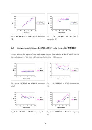
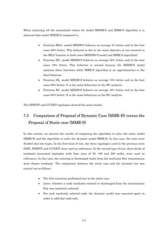
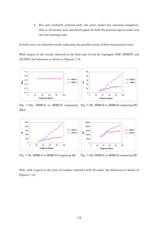
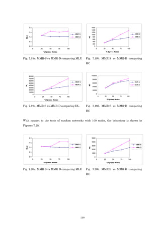
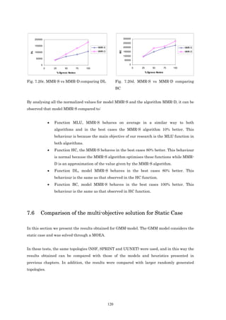

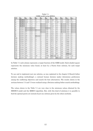
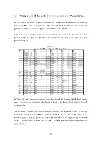
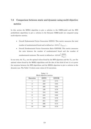


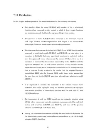


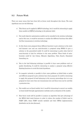
![References
[ABO98] E. Aboelela, C. Douligeris. “Fuzzy Generalized Network Approach for Solving an
Optimization Model for Routing in B-ISDN”. IEEE CCECE 1998/CCGEI 1998.
[ABR02] H. Abrahamsson, B. Ahlgren, J. Alonso, A. Andersson, P. Kreuger. “A Multi Path
Routing Algorithm for IP Networks based on Flow Optimisation”. LCNS 2511. QoFIS 2002.
[AHU97] R. Ahuja, M. Kodialam, A. Mishra, J. Orlin. “Theory and Methodology,
Computational Investigations of Maximum Flow Algorithms”. European Journal of
Operational Research. Published by Elsevier Science. 1997.
[AHU93] R. Ahuja, T. Magnanti, J. Orlin. “Network flows: Theory, algorithms and
applications”. Prentice-Hall. NJ. 1993.
[ALO02] S. Alouf, E. Altman, P. Nain. “Optimal on-line estimation of the size of a dynamic
multicast group”. IEEE Infocom. 2002.
[APP03] D. Applegate, M. Thorup. “Load optimal MPLS routing with N+M labels”. IEEE
INFOCOM 2003.
[ASH02] J. Ash, M. Girish, E. Gray, B. Jamoussi, G. Wright. “Applicability statement for CR-
LDP”. RFC 3213. Enero 2002.
[ASH02a] J. Ash, Y. Lee, P. Ashwood-Smith, B. Jamoussi, D. Fedyk, D. Skalecki, L. Li. “LSP
modification using CR-LDP”. RFC 3214. Enero 2002.
[AWD01] D. Awduche, L. Berger, D. Gan, T. Li, V. Srinivasan, G. Swallow. “RSVP-TE:
Extensions to RSVP for LSP tunnels”. RFC 3209. Diciembre 2001.
[BAC00] T. Back, D. Fogel, T. Michalewicz. “Evolutionary Computation 1”. IOP Publishing.
2000.
[BAL97] A. Ballardie. “Core Based Trees (CBT version 2) Multicast Routing”. RFC 2189.
Septiembre 1997.
132](https://image.slidesharecdn.com/programacionmultiobjetivo-121118123824-phpapp02/85/Programacion-multiobjetivo-152-320.jpg)
![[BAL97a] A. Ballardie. “Core Based Trees (CBT) Multicast Routing Architecture”. RFC 2201.
Septiembre 1997.
[BAN01] N. Banerjee, S. Das. “Fast Determination of QoS Multicast Routes in Wireless
Networks using Genetic Algorithm”. IEEE ICC 2001.
[BAR04] B. Baran, R. Fabregat, Y. Donoso, F. Solano, JL. Marzo. “Generalized Multiobjective
Multitree model”. Research Report Girona University 2004.
[BAZ90] M. Bazaraa, J. Jarvis, H. Sherali. “Linear Programming and Network Flows”. John
Wiley & Sons, 2nd ed, USA, 1990.
[BAZ93] M. Bazaraa, H. Sherali, C. Shetty. “Nonlinear Programming, Theory and Algorithms”.
John Wiley & Sons, 1993.
[BHA02] S. Bhatnagar, S. Ganguly, B. Nath. “Label space reduction in multipoint-to-point
LSPs for traffic engineering”. ECUMN2002.
[CAO00] Z. Cao, Z. Wang, E. Zegura. “Rainbow Fair Queueing: Fair Bandwidth Sharing
Without Per-Flow”. IEEE INFOCOM 2000.
[CAO00a] Z. Cao, Z. Wang, E. Zegura. “Performance of hashing-based schemes for Internet
load balancing”, IEEE INFOCOM 2000.
[CER04] S. Cerav-Erbas. “Traffic Engineering in MPLS Networks with Multiple Objectives:
Modeling and Optimization”. Thesis of Master of Science in Industrial and Systems
Engineering. Turkey. 2004.
[CET04] C. Cetinkaya, E. Knightly. “Opportunistic Traffic Scheduling Over Multiple Network
Paths”. IEEE INFOCOM 2004.
[CHA03] D. Chakraborty, G. Chakraborty, N. Shiratori. “A dynamic multicast routing
satisfying multiple QoS constraints”. International Journal of Network Management, John
Wiley & Sons. 2003.
133](https://image.slidesharecdn.com/programacionmultiobjetivo-121118123824-phpapp02/85/Programacion-multiobjetivo-153-320.jpg)
![[CHE01] J. Chen, S. Chan. "Multipath Routing for Video Unicast over Bandwidth-Limited
Networks". IEEE GLOBECOM 2001.
[CHO03] H. Cho, J. Lee, B. Kim. “Multi-path Constraint-based Routing Algorithms for MPLS
Traffic Engineering”. IEEE ICC 2003.
[COH78] J. Cohon. “Multiobjective programming and planning”. New York: Academic Press.
1978.
[COL03] Y. Collette, P. Siarry. “Multiobjective Optimization, Principles and Case Studies”.
Springer. 2003.
[CRI04] J. Crichigno, B. Barán. “A Multicast Routing Algorithm using Multiobjective
Optimization”. IEEE ICT 2004.
[CRI04a] J. Crichigno, B. Barán. “Multiobjective Multicast Routing Algorithm”. IEEE ICT
2004.
[CRI04b] J. Crichigno, B. Barán. “Multiobjective Multicast Routing Algorithm for Traffic
Engineering”. IEEE ICCCN 2004.
[CUI03] X. Cui, C. Lin, Y. Wei. “A Multiobjective Model for QoS Multicast Routing Based on
Genetic Algorithm”. ICCNMC 2003.
[CUI03a] Y. Cui, K. Xu, J. Wu. “Precomputation for Multi-constrained QoS Routing in High-
speed Networks”. IEEE INFOCOM 2003.
[DEB01] K. Deb. “Multi-Objective Optimiation using Evolutionary Algorithms”. John Wiley &
Sons. 2001.
[DEE98] Deering. “Protocol Independent Multicast Version 2 Dense Mode. Specification”.
draft-ietf-pim-v2-dm-01.txt. Noviembre 1998.
[DON03] Y. Donoso, R. Fabregat, L. Fàbrega. “Multi-Objective Scheme over Multi-Tree
Routing in Multicast MPLS Networks”. ACM/IFIP LANC 2003.
134](https://image.slidesharecdn.com/programacionmultiobjetivo-121118123824-phpapp02/85/Programacion-multiobjetivo-154-320.jpg)
![[DON03a] Y. Donoso, R. Fabregat. “Ingeniería de Tráfico aplicada a LSPs Punto-Multipunto
en Redes MPLS”. CLEI (Congreso Latinoamericano de Estudios en Informática) 2003. La Paz,
Bolivia. October 2003.
[DON04] Y. Donoso, R. Fabregat, JL. Marzo. “Multi-Objective Optimization Algorithm for
Multicast Routing with Traffic Engineering”. IEEE ICN 2004.
[DON04a] Y. Donoso, R. Fabregat, JL. Marzo. “Multi-Objective Optimization Model and
Heuristic Algorithm for Dynamic Multicast Routing”. IEEE & VDE Networks 2004.
[DON04b] Y. Donoso, R. Fabregat, JL. Marzo. “Multi-Objective Optimization Scheme for
Dynamic Multicast Groups”. IEEE ISCC 2004.
[DON04c] Y. Donoso, R. Fabregat, JL. Marzo. “Multi-Objective Optimization Algorithm for
Multicast Routing with Traffic Engineering.” Telecommunication Systems Journal. Kluwer
Publisher. 2004.
[DON04d] Y. Donoso, R. Fabregat, JL. Marzo. “Multi-Objective Optimization Model and
Heuristic Algorithm for Multipath Routing of Static and Dynamic Multicast Group.” III
Workshop on MPLS Networks. Girona, Spain. March 2004.
[DON04e] Y. Donoso, R. Fabregat, JL. Marzo. “Multicast Routing with Traffic Engineering: a
Multi-Objective Optimization Scheme and a Polynomial Shortest Path Tree Algorithm with
Load Balancing”. Proceedings of CCIO -2004 Cartagena de Indias, Colombia, March 2004.
[DON05] Y. Donoso, R. Fabregat, JL. Marzo. “Multicast Routing With Traffic Engineering: A
Multi-Objective Optimization Scheme And A Polynomial Shortest Path Tree Algorithm With
Load Balancing.” Annals of Operations Research. Kluwer Publisher. 2005.
[DON05a] Y. Donoso, R. Fabregat, F. Solano, JL. Marzo, B. Baran. “Generalized Multiobjective
Multitree model for Dynamic Multicast Groups”. IEEE ICC. Seoul. Korea. May 2005.
[EST98] D. Estrin. “Protocol Independent Multicast-Sparse Mode (PIM-SM): Protocol
Specification”. RFC 2362. Junio 1998.
[FAB04] R. Fabregat, Y. Donoso, F. Solano, JL. Marzo. “Multitree Routing for Multicast Flows:
A Genetic Algorithm Approach”. CCIA 2004.
135](https://image.slidesharecdn.com/programacionmultiobjetivo-121118123824-phpapp02/85/Programacion-multiobjetivo-155-320.jpg)
![[FAB04a] R. Fabregat, Y. Donoso, JL. Marzo, A. Ariza. “A Multi-Objective Multipath Routing
Algorithm for Multicast Flows”. SPECTS 2004.
[FOR02] B. Fortz, M. Thorup. “Optimizing OSPF/IS-IS weights in a changing world”. JSAC,
February 2002.
[GAM04] GAMS . Solver for large mathematical programming problems. http://www.gams.com
[GHA03] R. Ghanea-Hercock. “Applied Evolutionary Algorithms in Java”. Springer. 2003.
[GOL89] D. Goldberg. “Genetic Algorithms is Search, Optimization and Machine Learning”.
Addison-Wesley Publishing. 1989.
[GUP03] A. Gupta, A. Kumar, R. Rastogi. “Exploring the trade-off between label size and stack
depth in MPLS Routing”. IEEE INFOCOM 2003.
[HER03] R. Hernandez, C. Fernandez P. Baptista. “Metodología de la investigación”. Mc Graw
Hill. 3rd edition. 2003
[HOR97] J. Horn. “Multicriteria decision making and evolutionary computation”. InT. Baeck,
D. B. Fogel, and Z. Michalewicz, editors, Handbook of Evolutionary Computation. Institute of
Physics Publishing, Bristol, UK, 1997.
[IM95] Y. Im, Y. Lee, S. Wi, K. Lee, Y. Choi, C. Kim. “Multicast Routing Algorithms in Hihg
Speed Networks”. IEEE. 1995.
[INA99] J. Inagaki, M. Haseyama, H. Kitajima. “A Genetic Algorithm for Determining
Multiple Routes and its Applications”. Circuits and Systems, ISCAS 1999.
[IZM02] R. Izmailov, D. Niculescu. “Flow splitting approach for path provisioning and path
protection problems”. HPSR 2002.
[KIM02] C. Kim, Y. Choi, Y. Seok, Y. Lee. “A Constrained Multipath Traffic Engineering
Scheme for MPLS Networks”. IEEE ICC 2002.
136](https://image.slidesharecdn.com/programacionmultiobjetivo-121118123824-phpapp02/85/Programacion-multiobjetivo-156-320.jpg)
![[KIM04] J. Kim, C. Kim, S. Seok, C. Kang. “Traffic Engineering using Adaptive Multipath-
Forwarding Against Dynamic Traffic in MPLS Networks”. IEEE ICN 2004.
[KOY04] A. Koyama, L. Barolli, K. Matsumoto, B. Apduhan. “A GA-based Multi-purpose
Optimization Algorithm for QoS Routing”. IEEE AINA 2004.
[LAY04] L. Layuan, L. Chunlin. “QoS Multicast Routing in Networks with Uncertain
Parameter”. IEEE IPDPS 2004.
[LEE02] L. Lee, Y. Seok Y. Choi, C. Kim. “A Constrained Multipath Traffic Engineering
Scheme for MPLS Networks”. IEEE ICC 2002.
[LEU98] Y. Leung, G. Li, Z. Xu. “A Genetic Algorithm for the Multiple Destination Routing
Problems”. IEEE Transactions on Evolutionary Computation, Vol. 2, No. 4, November 1998.
[LI99] Y. Li, Y. Bouchebaba. “A new genetic algorithm for the optimal communication
spanning tree problem”. Proceedings of Artificial Evolution: Fifth European Conference. LNCS
1829. 1999.
[MED01] A. Medina, A. Lakhina, I. Mata, J. Byers. “BRITE: An Approach to Universal
Topology Generation”. In proceedings of the international workshop on modeling, analysis and
simulation of computer and telecommunications systems. 2001.
[MON04] D. Montgomery. “Diseño y Análisis de Experimentos”. Limusa Wiley. 2nd edition.
2004.
[MOY94] J. Moy. “Multicast Extensions to OSPF”. RFC 1584. Marzo 1994.
[OH03] Y. Oh, D. Kim, H. Yoen, M. Do, J. Lee. “Scalable MPLS multicast using label
aggregation in Internet broadcasting systems”. ICT 2003..
[POM04] D. Pompili, L. Lopez, C. Scoglio. “DIMRO: a DiffServ-Integrated Multicast algorithm
for Internet Resource Optimization in source specific multicast applications”. ICC 2004.
[PUS00] T. Pusateri. “Distance Vector Multicast Routing Protocol”. draft-ietf-idmr-dvmrp-v3-
10. Agosto 2000.
137](https://image.slidesharecdn.com/programacionmultiobjetivo-121118123824-phpapp02/85/Programacion-multiobjetivo-157-320.jpg)
![[RAG99] S. Raghavan, G Manimaran, C. Siva Ram Murthy. “A rearrangeagle algorithm for
the construction of delay-constrained dynamic multicast trees”. IEEE/ACM Transactions on
Networking, Vol. 7, Nº.4, pp. 514-529, August 1999
[RAO98] N. Rao, S. Batsell. “QoS Routing via multiple Paths using Bandwidth Reservation”.
IEEE INFOCOM 1998.
[ROS01] E. Rosen, A. Viswanathan, R. Callon. “Multiprotocol Label Switching Architecture”.
RFC 3031. 2001.
[ROY02] A. Roy, N. Banerjee, S. Das. “An Efficient Multi-Objective QoS-Routing Algorithm for
Wireless Multicasting”. IEEE INFOCOM 2002.
[ROY04] A. Roy, S. Das. “QM2RP: A QoS-based Mobile Multicast Routing Protocol using
Multi-Objective Genetic Algorithm”. The Journal of Mobile Communication, Computation and
Information, Wireless Networks. 2004.
[SAI00] H. Saito, Y. Miyao, M. Yoshida. “Traffic engineering using multiple multipoint-to-
point LSPs”. INFOCOM 2000.
[SEO02] Y. Seok, Y. Lee, Y. Choi, C. Kim. “Explicit Multicast Routing Algorithms for
Constrained Traffic Engineering”. IEEE ISCC 2002.
[SOL04] F. Solano, R. Fabregat, Y. Donoso. “Sub-flow assignment model of multicast flows
using multiple p2mp LSPs”. 30th Conferencia Latinoamericana de Informática (CLEI2004).
September 2004.
[SOL04a] F. Solano, R. Fabregat, Y. Donoso, JL. Marzo. “Mapping subflows to P2MP LSPs”.
IEEE International Workshop on IP Operations & Management (IPOM 2004). Beijing, China.
October 2004.
[SOL05] F. Solano, R. Fabregat, Y. Donoso, JL. Marzo. “Asymmetric Tunnels in P2MP LSPs as
a Label Space Reduction Method”. IEEE ICC 2005. Seoul, Korea. May 2005.
[SON03] J. Song, S. Kim, M. Lee, H. Lee, T. Suda. “Adaptive Load Distribution over Multipath
in MPLS Networks”. IEEE ICC 2003.
138](https://image.slidesharecdn.com/programacionmultiobjetivo-121118123824-phpapp02/85/Programacion-multiobjetivo-158-320.jpg)
![[SRI03] A. Sridharan, R. Guerin, C. Diot. “Achieving near-optimal traffic engineering solutions
for current OSPF/IS-IS networks”. IEEE INFOCOM 2003.
[STR02] A. Striegel, G. Manimaran. “A survey of QoS Multicasting Issues”. IEEE
Communications Magazine - June 2002.
[SUN99] Q. Sun. “A genetic algorithm for delay-constrained minimum-cost multicasting”.
Technical Report, IBR, TU Braunschweig, Butenweg, 74/75, 38106, 1999.
[THA00] D. Thaler. “Border Gateway Multicast Protocol (BGMP): Protocol Specification”.
draft-ietf-bgmp-spec-02.txt. Noviembre 2000.
[TRA03] H. Tran, R. Harris. “Genetic algorithm approach to rearrangement of QoS multicast
tree”. 3rd ATcrc Telecommunications & Networking Conference and Workshop, 11-12 Dec.
2003.
[VAN99] D. Van Veldhuizen. “Multiobjective Evolutionary Algorithms: Classifications,
Analysis and New Innovations”. Ph.D. Thesis. Air Force Institute of Technology. 1999.
[VIL99] C. Villamizar. “MPLS Optimized Multipath (MPLS-OMP)”. Internet Draft. 1999.
[VUT00] S. Vutukury, J. Garcia. “A traffic engineering approach based on minimum-delay
routing”. IEEE ICCN 2000.
[XIA99] F. Xiang, L. Junzhou, W. Jieyi, G. Guanqun. “QoS routing based on genetic
algorithm”. Computer Communications 22. pp. 1293-1399. May 1999.
[WAI88] D. Waitzman. “Distance Vector Multicast Routing Protocol”. RFC 1075. 1988.
[WAN01] Z. Wang. “Internet QoS. Arquitecture and Mechanism for Quality of Service”. Morgan
Kaufmann Publishers. 2001.
[WAN01a] Y. Wang, Z. Wang, L. Zhang. “Internet Traffic Engineering without Full Mesh
Overlaying”. INFOCOM 2001.
139](https://image.slidesharecdn.com/programacionmultiobjetivo-121118123824-phpapp02/85/Programacion-multiobjetivo-159-320.jpg)
![[ZIT99] E. Zitzler, L. Thiele. “Multiobjective Evolutionary Algorithm: A comparative case
study and the Strength Pareto Approach”. IEEE Transaction Evolutionary Computation.
Vol.3. No.4. 1999.
140](https://image.slidesharecdn.com/programacionmultiobjetivo-121118123824-phpapp02/85/Programacion-multiobjetivo-160-320.jpg)
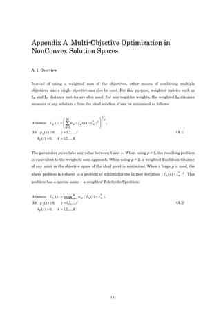
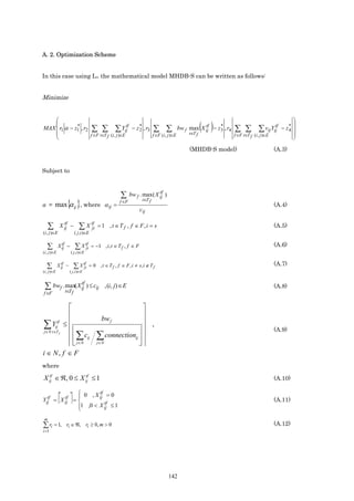


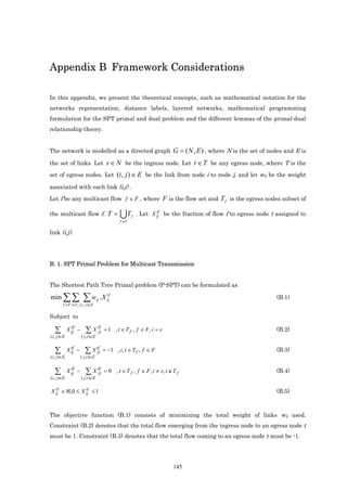
![Constraint (B.4) denotes that for any intermediate node which is different from the ingress
node, (i ≠ s), and from the egress nodes, (i ∉ T ) , the sum of their output flows to the egress
node t minus the input flows with a destination at the egress node t must be 0. Constraint
tf
(B.5) shows that the X ij variable may have a value of between 0 and 1. Solving the problem
without load balancing implies that this variable is only able to take the values 0 and 1, which
show respectively, whether the (i,j) link is or is not being used to carry information to the
egress node t.
tf
The solution using the X ij variables provides optimum flow values. These variables form the
multiple trees that transmit a multicast flow f from the ingress node to the set of egress nodes
Tf.
B. 2. Distance labels, layered networks and SPT Optimality Conditions
At this point, we will apply the concept of distance labels to the P-SPT problem.
+
A distance function d : N → Ζ U {0} with respect to a graph is a function from the set of
nodes N to the set of nonnegative integers. A distance function is valid with respect to a flow f
if it satisfies the following two conditions:
Lemma 1. d(s) = 0 and d(j) ≤ d(i) + 1 for every link (i,j) in graph G(N,E). d(i) is referred to as
the distance label of node i [AHU93], [AHU97], [BAZ90] and [BAZ93].
Lemma 2. If the conditions of the distance labels are valid, the distance label d(j) is a lower
bound on the length of the shortest (directed) path from node j to node s [AHU93], [AHU97],
[BAZ90] and [BAZ93].
Now, with respect to a given flow f, we can define the layered network G’(N,E) by determining
the exact distance labels d in G(N,E). The layered network consists of the links (i,j) in G(N,E)
satisfying the condition d(j) = d(i) + 1.
Let d tf for j ≠ s denote the length of a SPT from the ingress node to the egress nodes Tf. Thus,
j
tf
in keeping with lemma 1 and lemma 2, d s = 0, t ∈ T f , f ∈ F . If the distance labels are SPT
146](https://image.slidesharecdn.com/programacionmultiobjetivo-121118123824-phpapp02/85/Programacion-multiobjetivo-166-320.jpg)
![distances associated to the weights wij for each link (i,j), they must satisfy the following
optimality conditions:
Lemma 3 (SPT Optimality Conditions). Let λf be a tree from s to t, t ∈ T f , associated to the
flow f, which consists of several paths Pktf with 1≤k≤h, where h is the number of paths. For
every node j Є N in the tree, let d tf denote the length of a directed path in the path Pktf from
j
the ingress node to node j with a destination at the egress node t in the flow f. d tf represents
j
the SPT distances for all egress nodes to flow f if and only if they satisfy the following SPT
optimality conditions:
d tf ≤ d itf + wij , (i, j ) ∈ E , t ∈ T f , f ∈ F
j
tf
d s = 0, t ∈ T f , f ∈ F
B. 3. Mathematical programming duality theory
Each mathematical programming problem (P-Primal) is associated with another mathematical
programming problem (D-Dual). P and D are mathematically equivalent in the sense that they
have the same optimal objective value, and the optimal solution of D can be derived from the
optimal solution of P and, vice versa, due to the relationship of complementary slackness.
Lemma 4 (Weak duality). Let z(x) denote the objective function value of a feasible solution, x,
of the SPT problem and let β(d) denote the objective function value of a feasible solution of its
dual. Then β(d)≤ z(x) [AHU93].
The weak duality lemma implies that the objective function value of any dual feasible solution
is a lower bound of the objective function value of any primal feasible solution. One
consequence of this result is immediate: if a dual solution d and a primal solution x have the
same objective function value β ( d ) = z ( x ) , d must be an optimal solution of the dual problem
and x must be an optimal solution of the primal problem.
Lemma 5 (Strong duality). For any choice of problem, the SPT problem always has a solution
x and the dual SPT problem has a solution d satisfying the property that
β (d ) = z ( x ) [AHU93].
147](https://image.slidesharecdn.com/programacionmultiobjetivo-121118123824-phpapp02/85/Programacion-multiobjetivo-167-320.jpg)
![This lemma shows that any optimal solution, x , of the SPT problem always has an associated
dual solution, d , satisfying the condition β (d ) = z ( x ) . The weak and strong duality lemmas
imply several fundamental results concerning relationships between the primal and dual
problems. The following complementary slackness optimality conditions, which are another
way of relating the two problems, makes some of these relationships more explicit.
Lemma 6 (Complementary slackness optimality conditions) [AHU93]. If x is an optimal
solution of the primal SPT problem and d is an optimal solution of the dual SPT problem, the
pair ( x , d ) satisfies the complementary slackness optimality conditions:
If X ij > 0 , then d tf − d itf = wij .
tf
j
If Pktf is a path of the tree λf determined by X ij , (i, j ) ∈ E , t ∈ T f , f ∈ F , for each link
tf
(i, j ) ∈ Pktf , if X ij > 0 , then this implies that d tf − d itf = wij .
tf
j
B.4. Shortest Path Tree Dual Problem
Using the definition of the P-SPT problem and the concepts of the duality theory described
previously, in this section we demonstrate the relationship between the primal and dual SPT
problems.
The Shortest Path Tree Dual Problem (D-SPT) can be formulated as
max ∑ ∑ d ttf (B.6)
f ∈F t∈T f
Subject to
d tf − d itf ≤ wij , (i, j ) ∈ E , t ∈ T f , f ∈ F
j (B.7)
tf
By lemma 3 d s = 0, t ∈ T f , f ∈ F (B.8)
wij ≥ 0 (B.9)
tf tf
Let X ij be the optimal solution of (P-SPT). Then X ij determines the shortest path for each
egress node in a flow. Let d tf be the optimal solution of the dual problem (D-SPT). The values
j
of d tf can be viewed as the distance from the ingress node s to the node j based on the SPT to
j
the flow f with a destination at egress node t determined in (P-SPT). In particular,
d ttf , t ∈ T f , f ∈ F is the total length of the SPT from s to t, t ∈ T f . If d tf is any solution of
j
148](https://image.slidesharecdn.com/programacionmultiobjetivo-121118123824-phpapp02/85/Programacion-multiobjetivo-168-320.jpg)


![Appendix C Publications
Journals
• [DON05] Y. Donoso, R. Fabregat, JL. Marzo. “Multicast Routing With Traffic Engineering:
A Multi-Objective Optimization Scheme And A Polynomial Shortest Path Tree Algorithm
With Load Balancing.” Annals of Operations Research. Kluwer Publisher. 2005.
• [DON04c] Y. Donoso, R. Fabregat, JL. Marzo. “Multi-Objective Optimization Algorithm for
Multicast Routing with Traffic Engineering.” Telecommunication Systems Journal. Kluwer
Publisher. 2004.
International Conferences
• [DON05a] Y. Donoso, R. Fabregat, F. Solano, JL. Marzo, B. Baran. “Generalized
Multiobjective Multitree model for Dynamic Multicast Groups”. IEEE ICC. Seoul. Korea.
May 2005.
• [SOL05] F. Solano, R. Fabregat, Y. Donoso, JL. Marzo. “Asymmetric Tunnels in P2MP
LSPs as a Label Space Reduction Method”. IEEE ICC 2005. Seoul, Korea. May 2005.
• [SOL04a] F. Solano, R. Fabregat, Y. Donoso, JL. Marzo. “Mapping subflows to p2mp
LSPs”. IEEE International Workshop on IP Operations & Management (IPOM 2004).
Beijing, China. October 2004.
• [FAB04a] R. Fabregat, Y. Donoso, F. Solano, JL. Marzo. “Multitree Routing for Multicast
Flows: A Genetic Algorithm Approach”. Setè Congrés Català d’Intel·ligència Artificial
(CCIA’2004), Universitat Autònoma de Barcelona, Barcelona (Spain). October 2004.
• [SOL04] F. Solano, R. Fabregat, Y. Donoso. “Subflow assignment model of multicast flows
using multiple p2mp LSPs”. CLEI (Congreso Latinoamericano de Estudios en Informática)
2004. Arequipa, Perú. October 2004. Selected as Best Papers.
• [FAB04a] Y. Donoso, R. Fabregat, JL. Marzo, A. Ariza. “A Multi-Objective Multipath
Routing Algorithm for Multicast Flows.” International Symposium on Performance
155](https://image.slidesharecdn.com/programacionmultiobjetivo-121118123824-phpapp02/85/Programacion-multiobjetivo-175-320.jpg)
![Evaluation of Computer and Telecommunication Systems (SPECTS'04). San Jose, USA.
July 2004.
• [DON04a] Y. Donoso, R. Fabregat, JL. Marzo. “Multi-Objective Optimization Model and
Heuristic Algorithm for Dynamic Multicast Routing”. IEEE & VDE Networks 2004.
Vienna, Austria. June 2004.
• [DON04b] Y. Donoso, R. Fabregat, JL. Marzo. “Multi-Objective Optimization Scheme for
Dynamic Multicast Groups”. IEEE ISCC (The 9th IEEE Symposium on Computers and
Communications). Alexandria, Egypt. June 2004.
• [DON04] Y. Donoso, R. Fabregat, JL. Marzo. “Multi-Objective Optimization Algorithm for
Multicast Routing with Traffic Engineering”. IEEE 3rd International Conference on
Networking ICN'04, Guadeloupe, French Caribbean, March 2004. Selected as Best
Papers.
• [DON04d] Y. Donoso, R. Fabregat, JL. Marzo. “Multi-Objective Optimization Model and
Heuristic Algorithm for Multipath Routing of Static and Dynamic Multicast Group.” III
Workshop on MPLS Networks. Girona, Spain. March 2004.
• [DON04e] Y. Donoso, R. Fabregat, JL. Marzo. “Multicast Routing with Traffic
Engineering: a Multi-Objective Optimization Scheme and a Polynomial Shortest Path Tree
Algorithm with Load Balancing”. Proceedings of CCIO -2004 Cartagena de Indias,
Colombia, March 2004. Operation Research National Award given by the
Colombian Operations Research Society. March 2004.
• [DON03] Y. Donoso, R. Fabregat. “Multi-Objective Scheme over Multi-Tree Routing in
Multicast MPLS Networks”. IFIP/ACM Latin America Networking Conference 2003
(LANC03), IFIP-TC6 and ACM SIGCOMM, La Paz (Bolivia). October 2003.
• [DON03a] Y. Donoso, R. Fabregat. “Ingeniería de Tráfico aplicada a LSPs Punto-
Multipunto en Redes MPLS”. CLEI (Congreso Latinoamericano de Estudios en
Informática) 2003. La Paz, Bolivia. October 2003.
156](https://image.slidesharecdn.com/programacionmultiobjetivo-121118123824-phpapp02/85/Programacion-multiobjetivo-176-320.jpg)
![Research Reports
• [BAR04] B. Barán, R. Fabregat, Y. Donoso, F. Solano, JL. Marzo. “Generalized
Multiobjective Multitree model”. Proceedings of IIiA Research Report, ref. IIiA 04-08-RR,
Institut d'Informàtica i Aplicacions, University of Girona. September 2004.
157](https://image.slidesharecdn.com/programacionmultiobjetivo-121118123824-phpapp02/85/Programacion-multiobjetivo-177-320.jpg)

This PhD thesis presents multi-objective optimization schemes for static and dynamic multicast flows. For static multicast flows, an optimization model called MHDB-S is formulated that combines objectives like maximum link utilization, hop count, bandwidth consumption, and end-to-end delay. An algorithm called MMR-S is also proposed. For dynamic multicast flows where egress nodes can change, a model called MHDB-D is proposed that extends MHDB-S. The thesis also proposes a generalized multi-objective model called GMM and an algorithm using multi-objective evolutionary algorithms to solve it. Simulation results show the proposed schemes improve objectives over simplified models.