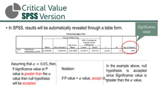
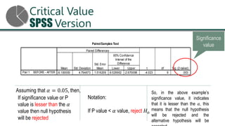
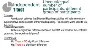
1) The document discusses various statistical analysis techniques that can be performed using the SPSS software, including Cronbach's alpha, t-tests (one sample, paired, and independent), ANOVA, ANCOVA, correlation, and regression analysis. 2) Examples are provided for each statistical technique to illustrate how to set up the analysis in SPSS, interpret the output and results, and make conclusions. 3) The examples cover topics in education and involve comparing groups, measuring relationships between variables, and predicting outcomes.

1. STATISTICAL ANALYSIS
THROUGH
STATISTICAL PACKAGE FOR THE SOCIAL SCIEN
(SPSS)
J A Y S O N B . B A L B I N

2. O
B
J
E
C
T
I
V
E
S
Determine the statistical
technique/method to be
used in a certain problem
Interpret generated
results from SPSS.
Perform data analysis through SPSS, specifically on:
• Cronbach’s Alpha
• One Sample T-test
• Paired T-test
• Independent T-test
• Analysis of Variance
• Analysis of Covariance
• Correlation
• Regression Analysis

3. H y p o t h e s i s T e s t i n g
Identify the variable
• Independent
• Dependent
Formulate Hypotheses
• Null
• Alternative
Identify the level
of
significance
Decision/
conclusion/
interpretation
Results
(in table form)
Test - statistics

4. Critical Value
SPSS Version
• In SPSS, results will be automatically revealed through a table form.
Paired Samples Test
-5.200000 7.405704 2.341889 -10.4977 .097721 -2.220 9 .054
FIRSTDAY -
ONEWEEKLATER
Pair
1
Mean Std. Deviation
Std. Error
Mean Lower Upper
95% Confidence
Interval of the
Difference
Paired Differences
t df Sig. (2-tailed)
Significance
value
Assuming that 𝛼 = 0.05, then,
If significance value or P
value is greater than the 𝛼
value then null hypothesis
will be accepted
Notation:
If P value > 𝛼 value, accept 𝐻𝑜
In the example above, null
hypothesis is accepted
since Significance value is
greater than the 𝛼 value.

5. Critical Value
SPSS Version
Significance
value
Assuming that 𝛼 = 0.05, then,
If significance value or P
value is lesser than the 𝛼
value then null hypothesis
will be rejected
Notation:
If P value < 𝛼 value, reject 𝐻𝑜
So, in the above example’s
significance value, it indicates
that it is lesser than the 𝑎, this
means that the null hypothesis
will be rejected and the
alternative hypothesis will be
PairedSamples Test
-6.100000 4.794673 1.516209 -9.529902 -2.670098 -4.023 9 .003
BEFORE - AFTER
Pair 1
Mean Std. Deviation
Std. Error
Mean Lower Upper
95% Confidence
Interval of the
Difference
Paired Differences
t df Sig. (2-tailed)

6. Cronbach’s
Alpha
A reliability coefficient
that provides a
method of measuring
INTERNAL
CONSISTENCY of
tests and measures.
If the instrument is
reliable, there should
be a great deal of
covariance among
items relative to the
Cronbach’s Alpha Interpretation
0.91 – 1.00 Excellent
0.81 – 0.90 Good
0.71 – 0.80 Good and
Acceptable
0.61 – 0.70 Acceptable
0.01 – 0.60 Non - Acceptable
Konting et al., 2009

7. T-test
A t-test is a type of inferential statistics
used to determine if there is a
significant difference between the
means of two groups, which may be
related in certain features.
3 types of T-Test
Paired T-test
One Sample T-
test
Independent T-
test
One Sample T-
test
Paired T-test
Independent T-
test
The one sample t-test is a statistical
hypothesis test used to determine whether
an unknown population mean is different
from a specific value.
A paired t-test is used when we are
interested in the difference between two
variables for the same subject.
Compares the means of two independent
groups in order to determine whether there
is statistical evidence that the associated
population means are significantly different.

8. One Sample
T-test
Example:
In the DepEd, it aims that every student should get at least 75 or higher
average to pass in a certain subject or in grade level
Research Question:
Is there a significant difference in the students grades from a standard
average of 75?
Hypotheses:
Ho: The grades of the students is equal to 75.
Ha: The grades of the students is greater than 75.
Compare a
Standard

9. Variable Standard Mean SD t – value p – value
GA 75 83.53 7.74 7.400 0.00
Suggested Tabular Presentation:
SPSS Result:

10. Decision/Interpretation:
With the obtained p-value of 0.00 which is lesser than the 𝑎- value of
0.05, this indicates that the null hypothesis will be rejected. Therefore, the
grades of the students is significantly higher than 75 as it is comparable
with the mean score of 83.53.

11. Paired
T-test
Example:
8th grade science class took the pre test on the solar system and then post
test after a week of class work learning the content.
Research Question:
Is there a significant difference between the pre-test and post test of the
students after a week of classwork learning the content?
Hypotheses:
Ho: There is NO significant difference between the pre-test and post test of the
students after a week of classwork learning the content
Ha: There is a significant difference between the pre-test and post test of the
students after a week of classwork learning the content
Pre-Post test;
the same
participants

12. Variable Mean SD t – value p – value
Pre Test 43.46 11.50 -2.541 0.018
Post Test 47.08 11.48
Suggested Tabular Presentation:
SPSS Result:

13. Decision/Interpretation:
With the obtained p-value of 0.018 which is lesser than the 𝑎- value of
0.05, this means that the null hypothesis will be rejected. Thus, there is a
significant difference between the pre-test and post test of the students after a
week of classwork learning the content. Post test obtained a mean of 47.08
which is significantly higher than the pre test of the students of just 43.46,
hence students performed better in the post test.

14. Independent
T-test
Example:
An educator believes that Directed Reading Activities will help elementary
pupils improve some aspects of their reading ability. Two sections were used to test
the claim.
Research Question:
Is there a significant difference between the DRA test result of the controlled
group and the experimental group?
Hypotheses:
Ho: There is NO significant difference.
Ha: There is a significant difference.
Unequal/equal
number of
participants; different
group of participants

15. Variable Mean SD t – value p – value
Experimental Group 51.48 11.01 2.267 0.029
Controlled Group 41.52 17.15
Suggested Tabular Presentation:
SPSS Result:

16. Decision/Interpretation:
With the obtained p-value of 0.026 which is lesser than the 𝑎-value of 0.05 this
means that null hypothesis will be rejected. Thus, there is a significant difference
between the Directed Reading Activity result of the experimental group and controlled
group. A mean score of 51.48 of experimental group’s DRA result concludes a better
performance than the controlled group with a mean score of only 41.52.

17. ANOVA
Analysis of Variance
ANOVA or Analysis of Variance is a
statistical test that determines a
significant difference between the
means of 3 or more independent
groups.
Example:
Do different brand of gasoline
affect mileage?

18. ANOVA
Analysis of Variance
Example:
Socio – Economic Status and Grades of Female Students
Research Question:
Is there a significant difference between the grades of female students with
different socio-economic status?
Hypotheses:
Ho: There is NO significant difference.
Ha: There is a significant difference.

19. Grades_SetA Mean SD f – value p – value
Low SES 88.58 4.25 0.728 0.49
Average SES 88.10 4.08
High SES 86.94 4.52
Suggested Tabular Presentation:
SPSS Result SET A:

20. Decision/Interpretation:
With the obtained p-value of 0.40 which is greater than the 𝑎- value of 0.00 the
null hypothesis is failed to be rejected (accepted), thus, it emphasizes that there is no
significant difference between the grades of the female students with different socio-
economic status. Female students’ academic performance is just the same despite
that they differ in terms of socio-economic status.

21. Grades_SetB Mean SD f – value p – value
Low SES 88.58 4.25 51.921 0.000
Average SES 77.11 1.94
High SES 86.94 4.52
Suggested Tabular Presentation:
SPSS Result SET B:

22. Decision/Interpretation:
With the obtained p-value of 0.00 which is greater than the 𝑎- value of 0.05 the
null hypothesis is rejected, hence, there is a significant difference between the
grades of the female students with different socio-economic status. It emphasizes
that high SES and low SES is significantly higher than the average SES.

23. Correlation
A CORRELATION COEFFICIENT
expresses the degree to which two
variables vary in the same or opposite
directions. Correlation coefficient
ranges from -1 to +1.
Correlation is a statistical technique
that tends to measure the relationship
of the values of two or more
quantitative variables.
Correlation Coefficient Relationship Interpretation
0.6 ≤ 𝑟 ≤ 1 Strong Positive Correlation Strong Positive
Relationship
0 < 𝑟 < 0.6 Weak Positive Correlation Weak Positive Relationship
𝑟 = 0 No Correlation No Relationship
−0.6 < 𝑟 < 0 Weak Negative Correlation Weak Negative
Relationship
−1 ≤ 𝑟 ≤ −0.6 Strong Negative
Correlation
Strong Negative
Relationship
Types of Correlation
• Pearson Correlation
• Spearman Rank Correlation

24. Pearson
Correlation
Example:
Relationship between time spent per day reading newspaper and scores in a
20 item recognition test.
Research Question:
Is there a significant relationship between their time spent reading newspaper
and their recognition test scores?
Hypotheses:
Ho: There is NO significant relationship.
Ha: There is a significant relationship.
Data is Interval or ratio
scale

25. r p – value
Time * Score 0.962 0.00
Suggested Tabular Presentation:
SPSS Pearson Result:

26. Decision/Interpretation:
With the obtained p value of 0.00 which is greater than the 𝑎-value of 0.05,
thus, the null hypothesis will be rejected. It indicates that there is a significant
relationship between time spent reading newspaper and scores in recognition test. With
a correlation coefficient of 0.962 it indicates a strong positive relationship.

27. Spearman
Correlation
Example:
An observer’s rate of attractiveness among 10 couples on a 10 point scale.
Research Question:
Is there a significant relationship in the given ratings of the observers?
Hypotheses:
Ho: There is NO significant relationship in the given ratings of the observers.
Ha: There is a significant relationship in the given ratings of the observers.
Ordinal scale

28. r p – value
Rating of Attractiveness 0.749 0.013
Suggested Tabular Presentation:
SPSS Spearman Result:
Decision/Interpretation:
Reject Ho (null hypotheses). Thus, there is a significant relationship in
the ratings given by the observers. A coefficient of 0.749, it indicates a
strong positive relationship.

29. Regression
A COEFFICIENT OF DETERMINATION
denoted by 𝑅2
(r squared) is the proportion of
the variation in the dependent variable that is
predictable from the independent variable.
Regression analysis examines the
relationship between two or more
variables of interest.
Regression formula
𝑌 = 𝐴 + 𝐵𝑋 + ⋯ + 𝐵𝑋𝑛
Where
Y = Dependent Variable
X = Independent Variable
A = intercept
B = slope

30. Regression
Analysis
Example:
Relationship between time spent per day reading newspaper and scores in a
20 item recognition test.
Research Question:
Does time spent per day reading newspaper predict the scores in a 20 item
recognition test?
Hypotheses:
Ho: Time spent reading newspaper does not predict recognition test scores.
Ha: Time spent reading newspaper predicts recognition test scores.

31. Variable r r square p – value
Time * scores 0.962 0.925 0.00
Suggested Tabular Presentation:
SPSS Regression Result:
Decision/Interpretation:
Reject Ho (null hypotheses). Therefore time spent reading newspaper
predicts recognition test score. The independent variable accounts
92.5% to the dependent variable.

32. The Regression Line Equation:
SPSS Regression Result:

33. 𝑦 = 3.67 + 0.25𝑥
What is the recognition test score of a student who spends 60 minutes reading newspap
𝑦 = 3.67 + 0.25(60)
𝑦 = 3.67 + 15
𝑦 = 18.67
𝑦 ≈ 19
Therefore, a student who spends 60 minutes reading newspaper will attain a score of 19

34. ANCOVA
Analysis of Covariance
ANCOVA is a statistical technique that
allows analyst to model the response of
a variable as a linear function of
predictor(s).
Example:
Examining the rate of learning of
different groups. The prior familiarity
of some students with the topics
leads to increased learning scores.
Inclusion of additional factors as a
statistical control to explain variation on
the dependent variable.

35. ANCOVA
Analysis of Covariance
Example:
Pre test and post test of Word Problem Solving Skills of two
sections(considered as experimental group and controlled group)
Research Question:
Is there a significant difference between experimental group and controlled
group in terms of their pre-test and post-test word problem solving skills?
Hypotheses:
Ho: There is NO significant difference.
Ha: There is a significant difference.

36. SPSS Result:

37. Group Mean SD N
Experimental Group 30.60 8.42 30
Controlled Group 25.33 8.13 30
Total 27.97 8.62 60
Source SS df MS F p-value
WPS_Pre-test 2144.716 1 2144.716 66.980 0.000
Group 203.792 1 203.792 6.364 0.014
Error 1825.150 57 32.020
Total 51314.00 60
Suggested Tabular Presentation:

38. Decision/Interpretation:
With the obtained p-value of 0.014 which is lesser than the 𝑎-value of 0.05, this
means that the null hypothesis will be rejected. Thus, there is a significant difference
between experimental and controlled group in terms of their pre-test and post-test in
word problem solving skills. Experimental group is performing better since their mean
is 30.60 than the controlled group with a mean of 25.33 only.

39. End
Jayson B. Balbin
Contact Information:
09161057855
09513801239
jeckbalbin@gmail.com