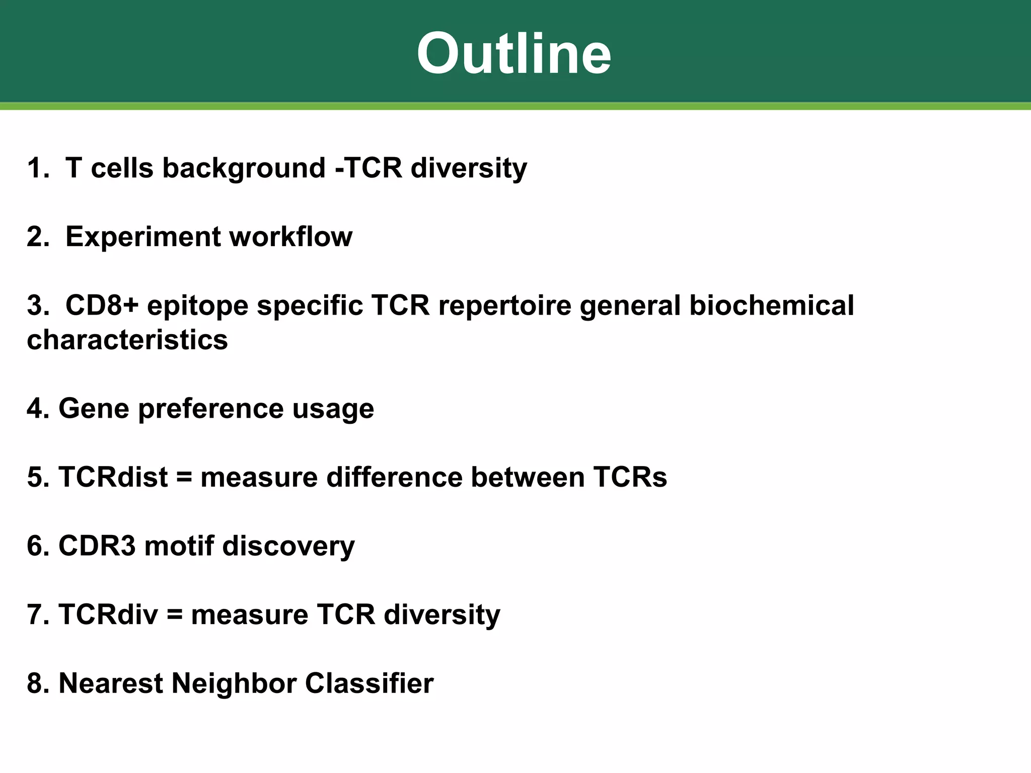
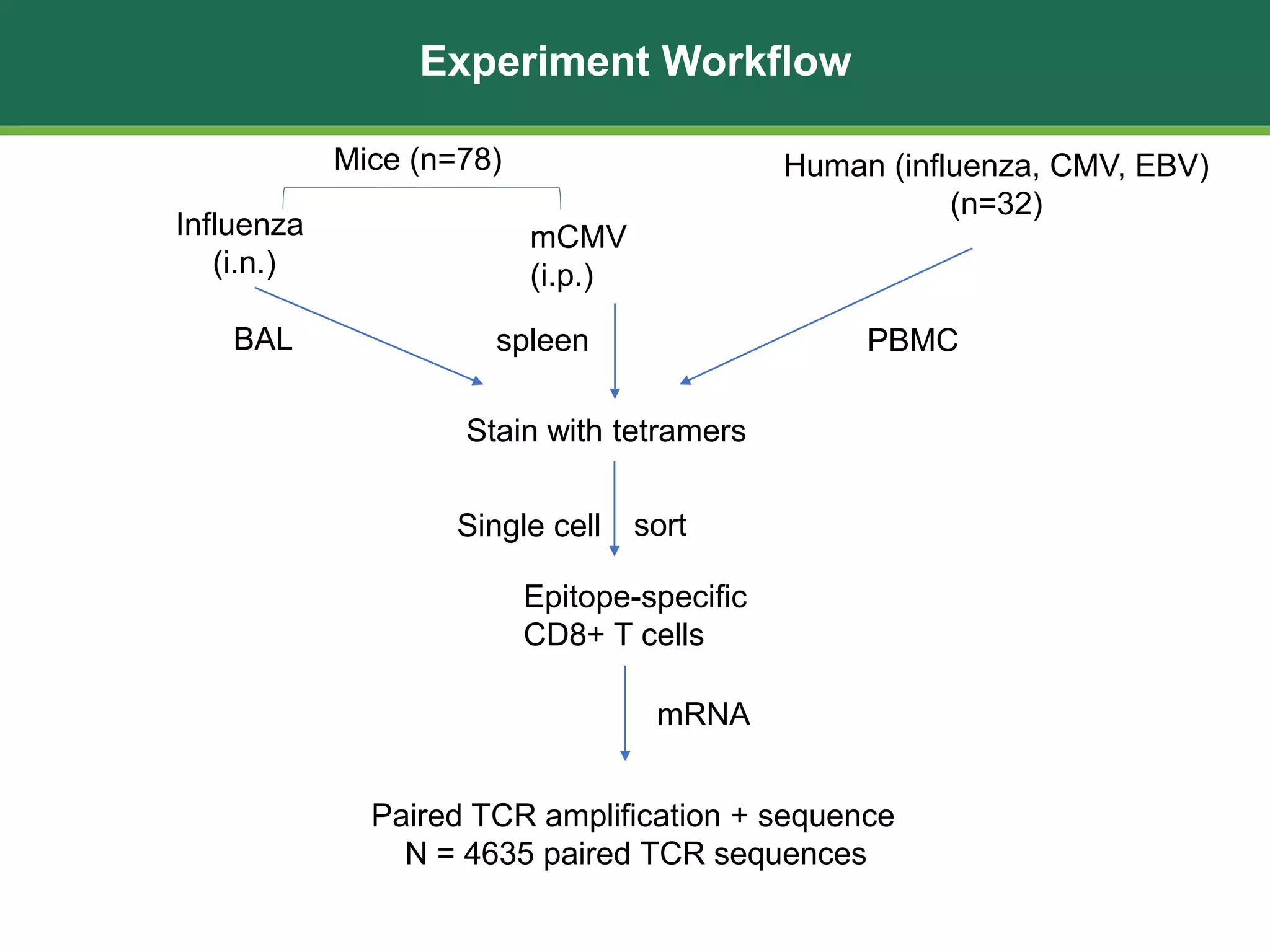
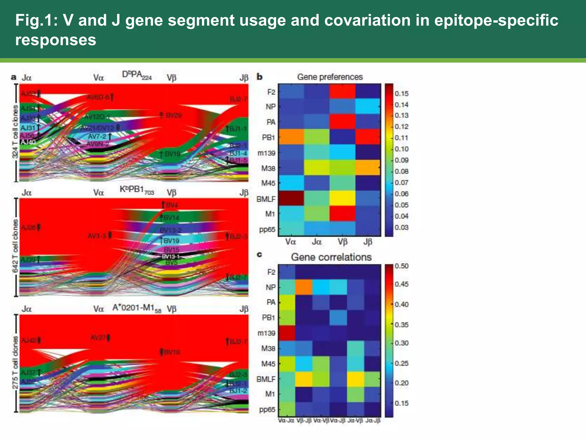
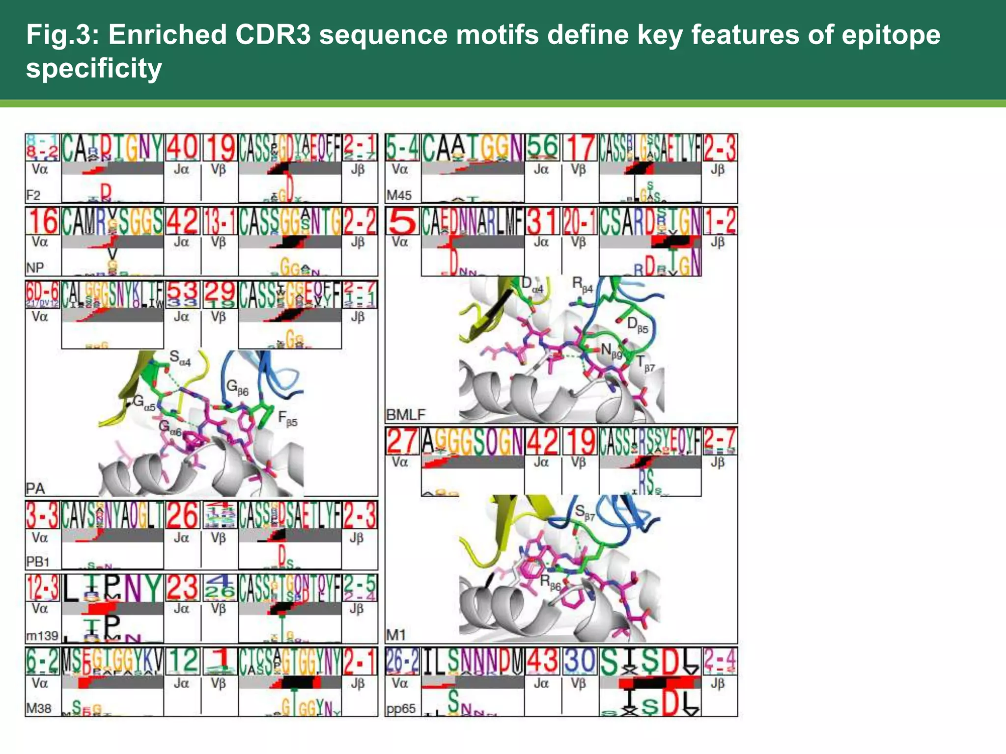
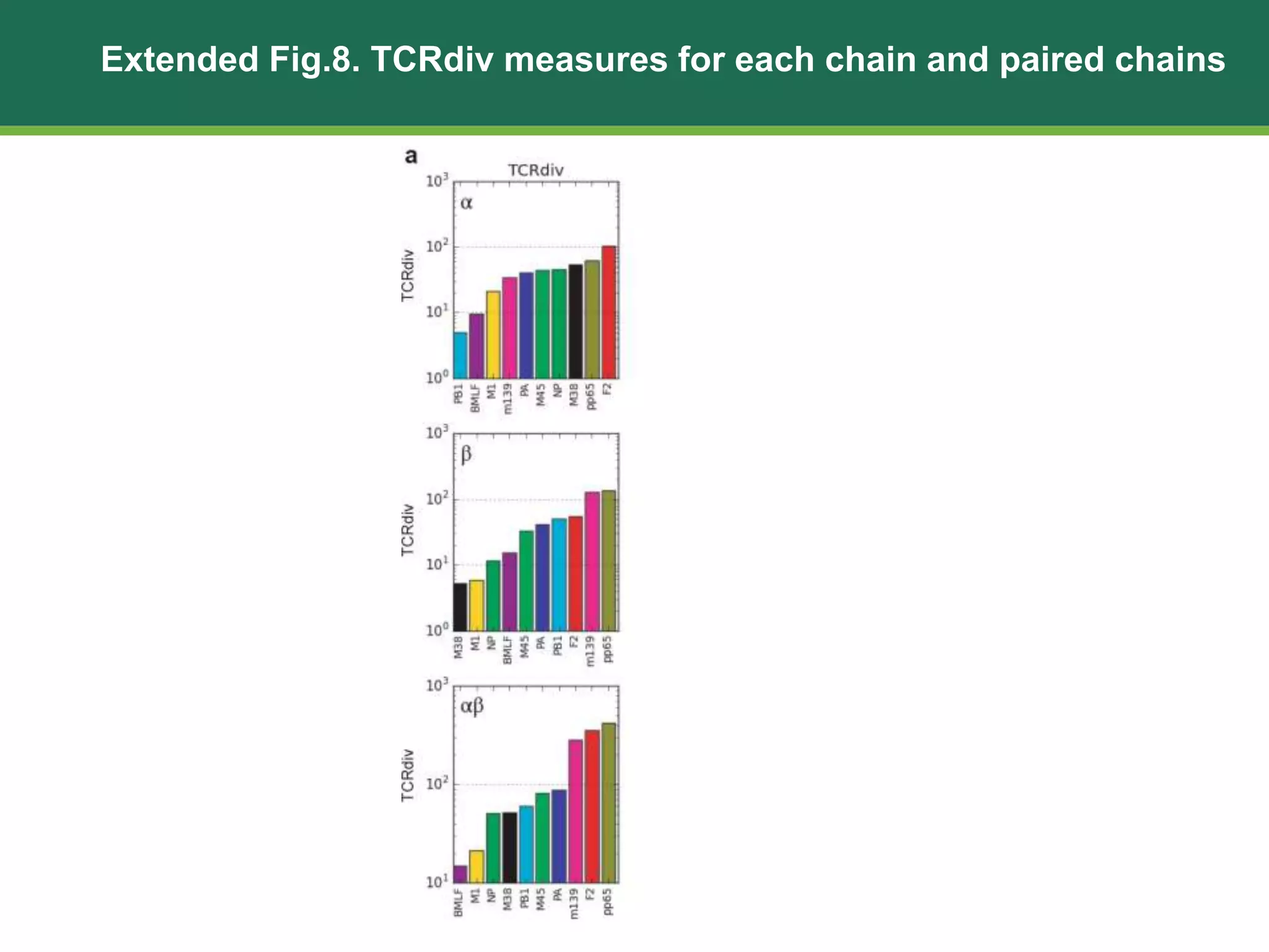
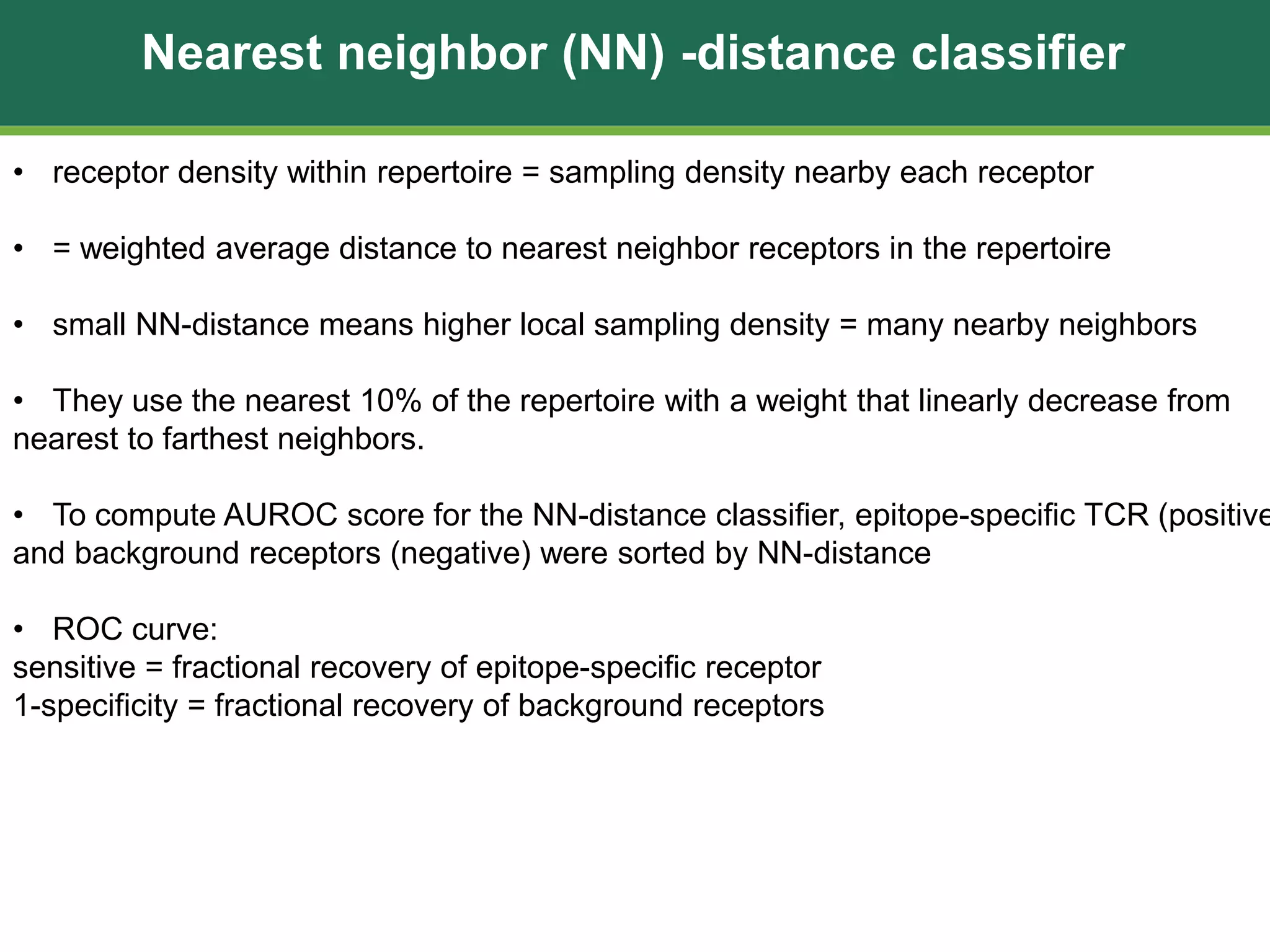
Quantifiable predictive features define
epitope-specific T cell receptor repertoires
Thi Nguyen, Ph.D. Candidate
Graduate Biomedical Sciences | Immunology Theme
University of Alabama at Birmingham (UAB)
kimthi@uab.edu
Summer Journal Club
August 29th, 2018
Outline
1. T cells background -TCR diversity
2. Experiment workflow
3. CD8+ epitope specific TCR repertoire general biochemical
characteristics
4. Gene preference usage
5. TCRdist = measure difference between TCRs
6. CDR3 motif discovery
7. TCRdiv = measure TCR diversity
8. Nearest Neighbor Classifier
T cells
• T cell/T lymphocyte, is a type of white blood cell that is critical for immune defense
• T cell can be distinguished from other leukocytes by the presence of TCR
• derived from hematopoietic stem cells in bone marrow
• mature in the thymus (thymocyte)
• have many different subsets with distinct function (helper, killer, regulatory)
• unique ability to recognize patterns between normal (self) vs abnormal (non-self or
cancerous or sick/dying) cells (cell-mediated immunity) through pMHC binding.
• Upon TCR-pMHC binding + costimulatory molecule binding, they become activated
• Depending on the cytokine cues from environment, they become differentiated
TCR diversity-V(D)J recommbination
Immunobiology: The Immune System in Health and Disease. 5th edition.
Janeway CA Jr, Travers P, Walport M, et al.
New York: Garland Science; 2001.
germline
• Theoretical estimate 1015 -1061 TCR
• Observed 106 TCR
Gene rearrangement
Experiment Workflow
Mice (n=78)
Influenza
(i.n.)
mCMV
(i.p.)
BAL
Stain with tetramers
sort
Epitope-specific
CD8+ T cells
spleen
Human (influenza, CMV, EBV)
(n=32)
Single cell
mRNA
Paired TCR amplification + sequence
N = 4635 paired TCR sequences
PBMC
Paired TCR𝛂𝝱 amplification and sequence
Pradyot Dash et al
Methods Mol. Biol. 2015
TCR𝛂𝝱 sequence analysis
• V and J genes were assigned using BLAST against the IMGT database
• CDR3 nucleotide and aa sequence were assigned based on the location of the
conserved cysteine in the V region and the FGXG motif in the J region.
• Full CDR3 starts at C104 and ending in F position of the FGXG motif
• trimmed CDR3 starts at the 3rd position after C104 and terminate with 2nd position
before F118
• To handle degenerate J-gene FGXG motifs, J aa sequence were manually aligned to
define the F118 position before sequence analysis
Extended table. TCR repertoires characteristics
clonality = 1 – Simpson’s diversity index
(normalized by the size of repertoire)
Pshare = estimated rate a clone drawn
from one subject has an identical
aa sequence to another subject
Extended Fig.1. CDR3 region characteristics of 10 epitope-specific TCR repertoires
How do they quantify gene preference?
Jensen-Shannon divergence (JSD) (total divergence to the average)
• measure the similarity between two probability distribution/ quantifies how
distinguishable two distributions are from each other.
• Based on Kullback-Leibler divergence but it is symmetric and has a finite value
• Basic form = entropy of the mixture minus the mixture of the entropy
Gene usage preference = a normalized JSD between gene frequencies of epitope-
specific repertoire and non-specific background from public dataset.
• This can be generalized to a number of random variables with arbitrary weights:
Gene correlation analysis
• covariation between gene usage was quantified by adjusted mutual information
• correct for the number and frequencies of the observed genes that cluster by chance
• set lower significance threshold in Fig.1c, they randomly shuffled genes in each of
the 60 gene pairing lists 100 times and recompute the adjusted mutual information.
• The largest value observed in these 6000 random trials = lower significance threshold
Fig.1: V and J gene segment usage and covariation in epitope-specific
responses
Extended Data Figure 2: V and J gene segment usage and covariation
in epitope-specific responses
Extended Data Figure 3. Schematic overview of the TCRdist
• Similarity between TCR = similarity between pMHC-
contacting loops.
• Loops are defined based on IMGT CDR
definition with modifications:
(1) Include CDR2.5
(2) Use trimmed CDR3
• AAdist (Alignment score) = BLOSUM62 matrix
• TCRdist = Sum (weighted AAdist)
distance(a,a) = 0
distance(a,b) = min (4, 4-BLOSUM62(a,b) to reduce
penalty for aa with positive BLOSUM62 score.
• A gap penalty of 4 (8 for CDR3) = distance between
gap position and an aa.
• Weight of 3 is applied to mismatches in the CDR3.
BLOSUM62 matrix
BLOSUM = Block substitution matrix
• Score alignment between protein sequence (locally , as opposed to PAM)
• Based on observed alignments
• Larger = higher sequence similarity => smaller evolutionary distance
Clustering and dimensionality reduction
• TCR with the largest number of neighbors within the distance threshold is chosen
as a cluster center.
 It and all its neighbors are removed from the repertoires
 repeat the process until all TCRs have been clustered.
• The distance threshold was chosen to yield homogeneous cluster of sufficient size,
same threshold was used for all repertoire
• result of this clustering method was visualized by average-linkage hierarchical clusterin
trees and TCR sequence logos
• They also use 2D kernel PCA (scikit-learn, KernelPCA function) to visualize the TCR
landscape. This attempts to preserve similarity structure of the input data while reducing
their dimensionality.
Fig.2: TCRdist analysis of the M45 repertoire identifies clusters of
related receptors
TCR logos
• summarize V and J gene usage, CDR3 aa sequence
and inferred rearrangement structure of the CDR3
• 4 components:
1. V-gene logos (left): V-gene names are scaled by
frequency and stacked top to bottom from most to least
common
2. CDR3 sequence logo where aa are scaled and ordered
by frequency and colored by chemical type.
3. a J-gene logo (right)
4. CDR3 where the genomic source regions for each
nucleotide column are represented by frequency-scaled
bars ordered top to bottom from V to D to J and colored
according to their frequency.
Extended Fig.4:
2D projections of mouse epitope-specific TCR repertoire
• kernel PCA applied to TCRdist
• Colored based on gene segment usage
kernel PCA ~ nonlinear form of PCA
CDR3 motif discovery
• Motifs = fixed length patterns consisting of aa position, wild card positions, aa group
positions (allowed groupings (K,R), (D, E), (N,Q), (S,T), (FYWH), (AGSP), (VILM))
• motif score = (observed –expected)2 /expected.
• observed = number of times motifs were observed from TCR sequence
• expected = values from background TCR (with V and J gene match observed repertoire
• Starting with two-position motifs scoring above a seed threshold, each motif was
iteratively extended by adding new specified position that increase the motif score.
• motif scores were sorted and filtered for redundancy.
• motif score above a threshold were extended to include near-neighbour TCR using
a stringent distance threshold => capture additional patterns
• final set of motif for each repertoire were visualized using TCR logo.
Amino Acid Groupings
https://en.wikipedia.org/wiki/Amino_acid
Fig.3: Enriched CDR3 sequence motifs define key features of epitope
specificity
TCRdiv metric to measure repertoire diversity
Simpson diversity index (D):
• takes into account of both the
richness and evenness of the
population.
• Measure the probability that 2
Individuals randomly selected from
A population will belong to the same class.
• 0 ≤ D ≤ 1
• 1 means the samples are identical
• 0 means otherwise
TCRdiv:
• Estimate the expected value of a Gaussian function of the inter-sample that returns
1 if the samples are identical and exp(-(TCRdist(a,b)/s.d.)2) otherwise.
• S.d. = 18.45 for single chain distance and twice that for paired analyses based on
empirical assessments of receptor distance distribution for multiple epitopes.
• TCRdiv =inverse of this estimate
http://www.countrysideinfo.co.uk/simpsons.htm
Extended Fig.8. TCRdiv measures for each chain and paired chains
Nearest neighbor (NN) -distance classifier
• receptor density within repertoire = sampling density nearby each receptor
• = weighted average distance to nearest neighbor receptors in the repertoire
• small NN-distance means higher local sampling density = many nearby neighbors
• They use the nearest 10% of the repertoire with a weight that linearly decrease from
nearest to farthest neighbors.
• To compute AUROC score for the NN-distance classifier, epitope-specific TCR (positive
and background receptors (negative) were sorted by NN-distance
• ROC curve:
sensitive = fractional recovery of epitope-specific receptor
1-specificity = fractional recovery of background receptors
Nearest Neighbor Classifiers
http://user.it.uu.se/~kostis/Teaching/DM-05/Slides/classification01.pdf
KNN algorithm
http://user.it.uu.se/~kostis/Teaching/DM-05/Slides/classification01.pdf
Fig.4 . Quantifying the defining features of epitope-specific populations
Extended Fig 9. Specificity and Avidity of the dispersed TCR
Modeling gene rearrangement
• Each nucleotide of the CDR3 is assigned to either V, D, J or N-nucleotide insertion
so as to minimize number of N.
• They sample V and J gene segments from the observed receptors but generated
the junctional sequences based on the inferred probability distribution for number of
insertion and deletion from the background TCR (public data).
• They also use these probability distributions to generate the random receptors that
formed one of the two control set for CDR3 motif discovery algorithm.
extended Fig.8.
Summary
• characterize 10 epitope-specific TCR repertoires of CD8+ T cells from 4600 single
celled TCR:
 gene segment usage
 epitope selection
• Develop TCRdist to quantify similarity among TCR based on spaces of TCR
• Develop TCRdiv to quantify TCR repertoire diversity
• develop a distance-based classifier that can assign unobserved TCR to characterized
TCR
Significance:
• potential application to analyze clinical TCR repertoire data where the target is
unknown such as in TIL.
• propose that despite tremendous diversity of TCR, we can develop predictive model for
TCR-pMHC recognition.

Predictive Features of TCR Repertoire

  • 1.
    Quantifiable predictive featuresdefine epitope-specific T cell receptor repertoires Thi Nguyen, Ph.D. Candidate Graduate Biomedical Sciences | Immunology Theme University of Alabama at Birmingham (UAB) kimthi@uab.edu Summer Journal Club August 29th, 2018
  • 2.
    Outline 1. T cellsbackground -TCR diversity 2. Experiment workflow 3. CD8+ epitope specific TCR repertoire general biochemical characteristics 4. Gene preference usage 5. TCRdist = measure difference between TCRs 6. CDR3 motif discovery 7. TCRdiv = measure TCR diversity 8. Nearest Neighbor Classifier
  • 3.
    T cells • Tcell/T lymphocyte, is a type of white blood cell that is critical for immune defense • T cell can be distinguished from other leukocytes by the presence of TCR • derived from hematopoietic stem cells in bone marrow • mature in the thymus (thymocyte) • have many different subsets with distinct function (helper, killer, regulatory) • unique ability to recognize patterns between normal (self) vs abnormal (non-self or cancerous or sick/dying) cells (cell-mediated immunity) through pMHC binding. • Upon TCR-pMHC binding + costimulatory molecule binding, they become activated • Depending on the cytokine cues from environment, they become differentiated
  • 4.
    TCR diversity-V(D)J recommbination Immunobiology:The Immune System in Health and Disease. 5th edition. Janeway CA Jr, Travers P, Walport M, et al. New York: Garland Science; 2001. germline • Theoretical estimate 1015 -1061 TCR • Observed 106 TCR Gene rearrangement
  • 5.
    Experiment Workflow Mice (n=78) Influenza (i.n.) mCMV (i.p.) BAL Stainwith tetramers sort Epitope-specific CD8+ T cells spleen Human (influenza, CMV, EBV) (n=32) Single cell mRNA Paired TCR amplification + sequence N = 4635 paired TCR sequences PBMC
  • 6.
    Paired TCR𝛂𝝱 amplificationand sequence Pradyot Dash et al Methods Mol. Biol. 2015
  • 7.
    TCR𝛂𝝱 sequence analysis •V and J genes were assigned using BLAST against the IMGT database • CDR3 nucleotide and aa sequence were assigned based on the location of the conserved cysteine in the V region and the FGXG motif in the J region. • Full CDR3 starts at C104 and ending in F position of the FGXG motif • trimmed CDR3 starts at the 3rd position after C104 and terminate with 2nd position before F118 • To handle degenerate J-gene FGXG motifs, J aa sequence were manually aligned to define the F118 position before sequence analysis
  • 8.
    Extended table. TCRrepertoires characteristics clonality = 1 – Simpson’s diversity index (normalized by the size of repertoire) Pshare = estimated rate a clone drawn from one subject has an identical aa sequence to another subject
  • 9.
    Extended Fig.1. CDR3region characteristics of 10 epitope-specific TCR repertoires
  • 10.
    How do theyquantify gene preference? Jensen-Shannon divergence (JSD) (total divergence to the average) • measure the similarity between two probability distribution/ quantifies how distinguishable two distributions are from each other. • Based on Kullback-Leibler divergence but it is symmetric and has a finite value • Basic form = entropy of the mixture minus the mixture of the entropy Gene usage preference = a normalized JSD between gene frequencies of epitope- specific repertoire and non-specific background from public dataset. • This can be generalized to a number of random variables with arbitrary weights:
  • 11.
    Gene correlation analysis •covariation between gene usage was quantified by adjusted mutual information • correct for the number and frequencies of the observed genes that cluster by chance • set lower significance threshold in Fig.1c, they randomly shuffled genes in each of the 60 gene pairing lists 100 times and recompute the adjusted mutual information. • The largest value observed in these 6000 random trials = lower significance threshold
  • 12.
    Fig.1: V andJ gene segment usage and covariation in epitope-specific responses
  • 13.
    Extended Data Figure2: V and J gene segment usage and covariation in epitope-specific responses
  • 14.
    Extended Data Figure3. Schematic overview of the TCRdist • Similarity between TCR = similarity between pMHC- contacting loops. • Loops are defined based on IMGT CDR definition with modifications: (1) Include CDR2.5 (2) Use trimmed CDR3 • AAdist (Alignment score) = BLOSUM62 matrix • TCRdist = Sum (weighted AAdist) distance(a,a) = 0 distance(a,b) = min (4, 4-BLOSUM62(a,b) to reduce penalty for aa with positive BLOSUM62 score. • A gap penalty of 4 (8 for CDR3) = distance between gap position and an aa. • Weight of 3 is applied to mismatches in the CDR3.
  • 15.
    BLOSUM62 matrix BLOSUM =Block substitution matrix • Score alignment between protein sequence (locally , as opposed to PAM) • Based on observed alignments • Larger = higher sequence similarity => smaller evolutionary distance
  • 16.
    Clustering and dimensionalityreduction • TCR with the largest number of neighbors within the distance threshold is chosen as a cluster center.  It and all its neighbors are removed from the repertoires  repeat the process until all TCRs have been clustered. • The distance threshold was chosen to yield homogeneous cluster of sufficient size, same threshold was used for all repertoire • result of this clustering method was visualized by average-linkage hierarchical clusterin trees and TCR sequence logos • They also use 2D kernel PCA (scikit-learn, KernelPCA function) to visualize the TCR landscape. This attempts to preserve similarity structure of the input data while reducing their dimensionality.
  • 17.
    Fig.2: TCRdist analysisof the M45 repertoire identifies clusters of related receptors TCR logos • summarize V and J gene usage, CDR3 aa sequence and inferred rearrangement structure of the CDR3 • 4 components: 1. V-gene logos (left): V-gene names are scaled by frequency and stacked top to bottom from most to least common 2. CDR3 sequence logo where aa are scaled and ordered by frequency and colored by chemical type. 3. a J-gene logo (right) 4. CDR3 where the genomic source regions for each nucleotide column are represented by frequency-scaled bars ordered top to bottom from V to D to J and colored according to their frequency.
  • 18.
    Extended Fig.4: 2D projectionsof mouse epitope-specific TCR repertoire • kernel PCA applied to TCRdist • Colored based on gene segment usage kernel PCA ~ nonlinear form of PCA
  • 19.
    CDR3 motif discovery •Motifs = fixed length patterns consisting of aa position, wild card positions, aa group positions (allowed groupings (K,R), (D, E), (N,Q), (S,T), (FYWH), (AGSP), (VILM)) • motif score = (observed –expected)2 /expected. • observed = number of times motifs were observed from TCR sequence • expected = values from background TCR (with V and J gene match observed repertoire • Starting with two-position motifs scoring above a seed threshold, each motif was iteratively extended by adding new specified position that increase the motif score. • motif scores were sorted and filtered for redundancy. • motif score above a threshold were extended to include near-neighbour TCR using a stringent distance threshold => capture additional patterns • final set of motif for each repertoire were visualized using TCR logo.
  • 20.
  • 21.
    Fig.3: Enriched CDR3sequence motifs define key features of epitope specificity
  • 22.
    TCRdiv metric tomeasure repertoire diversity Simpson diversity index (D): • takes into account of both the richness and evenness of the population. • Measure the probability that 2 Individuals randomly selected from A population will belong to the same class. • 0 ≤ D ≤ 1 • 1 means the samples are identical • 0 means otherwise TCRdiv: • Estimate the expected value of a Gaussian function of the inter-sample that returns 1 if the samples are identical and exp(-(TCRdist(a,b)/s.d.)2) otherwise. • S.d. = 18.45 for single chain distance and twice that for paired analyses based on empirical assessments of receptor distance distribution for multiple epitopes. • TCRdiv =inverse of this estimate http://www.countrysideinfo.co.uk/simpsons.htm
  • 23.
    Extended Fig.8. TCRdivmeasures for each chain and paired chains
  • 24.
    Nearest neighbor (NN)-distance classifier • receptor density within repertoire = sampling density nearby each receptor • = weighted average distance to nearest neighbor receptors in the repertoire • small NN-distance means higher local sampling density = many nearby neighbors • They use the nearest 10% of the repertoire with a weight that linearly decrease from nearest to farthest neighbors. • To compute AUROC score for the NN-distance classifier, epitope-specific TCR (positive and background receptors (negative) were sorted by NN-distance • ROC curve: sensitive = fractional recovery of epitope-specific receptor 1-specificity = fractional recovery of background receptors
  • 25.
  • 26.
  • 27.
    Fig.4 . Quantifyingthe defining features of epitope-specific populations
  • 28.
    Extended Fig 9.Specificity and Avidity of the dispersed TCR
  • 29.
    Modeling gene rearrangement •Each nucleotide of the CDR3 is assigned to either V, D, J or N-nucleotide insertion so as to minimize number of N. • They sample V and J gene segments from the observed receptors but generated the junctional sequences based on the inferred probability distribution for number of insertion and deletion from the background TCR (public data). • They also use these probability distributions to generate the random receptors that formed one of the two control set for CDR3 motif discovery algorithm. extended Fig.8.
  • 30.
    Summary • characterize 10epitope-specific TCR repertoires of CD8+ T cells from 4600 single celled TCR:  gene segment usage  epitope selection • Develop TCRdist to quantify similarity among TCR based on spaces of TCR • Develop TCRdiv to quantify TCR repertoire diversity • develop a distance-based classifier that can assign unobserved TCR to characterized TCR Significance: • potential application to analyze clinical TCR repertoire data where the target is unknown such as in TIL. • propose that despite tremendous diversity of TCR, we can develop predictive model for TCR-pMHC recognition.

Editor's Notes

  • #5 TCR is heterodimeric surface receptor that mediates recognition of pathogens-associated epitope through interaction with pMHC. TCR are generagted by genomic rearrangement of germline TCR locus, a process called VDJ that has the potential to generate marked diversity of TCR, estimated from. However, only observed 106 TCR due to several limitation (biological, experimental, technical). This cartoon on left show the germline organization of the human T-cell receptor α and β loci:  cluster of 61 Jα gene segments is located a considerable distance from the Vα gene segments. The Jα gene segments are followed by a single C gene, which contains separate exons for the constant and hinge domains and a single exon encoding the transmembrane and cytoplasmic regions. The TCRβ locus (chromosome 7) has a different organization, with a cluster of 52 functional Vβ gene segments located distantly from two separate clusters each containing a single D gene segment, together with six or seven J gene segments and a single C gene. Each TCRβ C gene has separate exons encoding the constant domain, the hinge, the transmembrane region, and the cytoplasmic region (not shown). The TCRα- and β-chain genes are composed of discrete segments that are joined by somatic recombination during development of the T cell. For the α chain, a Vα gene segment rearranges to a Jα gene segment to create a functional V-region exon. Transcription and splicing of the VJα exon to Cα generates the mRNA that is translated to yield the T-cell receptor α-chain protein. For the β chain, the variable domain is encoded in three gene segments, Vβ, Dβ, and Jβ. Rearrangement of these gene segments generates a functional VDJβ V-region exon that is transcribed and spliced to join to Cβ; the resulting mRNA is translated to yield the T-cell receptor β chain. The α and β chains pair soon after their biosynthesis to yield the α:β T-cell receptor heterodimer, that can bind to a particular pMHC presented by APC. Now TCR that recognize the same pMHC molecular more often than not have completely different sequences. But for the most part, they also have certain similarity. This paper attempt to characterize the similarity and different of unique different TCR from TCR repertoire that are epitope specific, hoping that this will enable them to predictively model TCR sequence given known epitope and vice versa. Say, given a particular TCR sequence, we’re going to predict the pMHC it bind to.
  • #7 Historically studying the real TCR sequence in repertoire is impossible because of bulk sequencing. Now with recent advance in single cell sequencing, the possibility to study and model TCR and immune response is endless. First, they use flow cytometry to sort for CD8 T cells that are specific to certain epitope of virus by staining cells in pMHC-tetramer. After single cell sort, they subject these cells to paired TCR amplification, first, isolate RNA then make cDNA and do 2 rounds of nested PCR to amplify CDR3alpha and beta parralellely. Then they sequence these PCR products-> translate to aa sequence then combine alpha with beta to have the alphabeta coexpression profile.
  • #8 Degeneracy of genetic code = different nucleotide sequence encode the same polypeptide.
  • #9 They first analyze this TCR repertoire data set using established feature such as length, charge, hydrophobicity. a, TCR repertoires of 10 epitope-specific populations. Where as there are substantial levels of sharing or publicity were observed at the single chain level, lower level of sharing was observed, with 3 epitops (F2,m139 and pp65) have no public receptor in this data set. b, Biophysical characteristics of TCR repertoires of 10 epitope specific populations.
  • #10 CDR3 length, charge, hydrophobicity, and inferred number of junctional nucleotide insertions for both single and paired chains as shown in the histograms. Different epitopes are colour-coded. Gere show that mean values for CDR3 length, charge and hydrophobicity are tightly clustered for the majority of the epitopes and all these features show great degree of overlapping ranges. B. Correlation between CDR3α β and antigenic peptides for charge, hydrophobicity, length, and N-insertions observed in all 10 epitopes. They found a negative correlation between CDR3 charge and peptide charge, peptide length and CDR3 length, suggesting that charge and length complemetarity may have a role in pMHC recognition.
  • #11 To quantify gene preference, they constructed a background, non-epitope selected repertoire by combining public data and compare gene frequencies between epitope-specific repertoire to those seen in background set.
  • #13 Fig 1 A . Gene segment usage and gene–gene pairing landscapes are illustrated graphically using four vertical stacks (one for each V and J segment) connected by curved segments with thickness proportional to the number of TCRs with the respective gene pairing (each panel is labelled with the four gene segments atop their respective colour stacks and the epitope identifier in the top middle). Genes are coloured by frequency within the repertoire with a fixed colour sequence used throughout the manuscript which begins red (most frequent),green (second most frequent), blue, cyan, magenta, and black. Clonallyexpanded TCRs were reduced to a single data point for this analysis. Thenumber of clones is indicated to the left of each panel. The enrichment of gene segments relative to background frequencies is indicated by up or down arrows, with each successive arrowhead corresponding to an additional twofold deviation. A shows the degree of dominance of single gene and pairwise gene associations. Each epitope specific response is characterized by an overrepresentation of individual genes as well as gene pairing preferences. Example is PB1 epitope, where Trav3-3, Tra26 and Trb2-3 are used in the single largest block of receptors. B. Jensen-Shannon divergence between observed gene usage of the epitope-specific CD8+ T cell repertoire compared to background, normalized by mean Shannon entropy. Higher value show higher gene preference. C.. Show gene usage correlation between V and J segment within a chain or across chain
  • #14 Gene segment usage and gene–gene pairing landscapes are illustrated graphically using four vertical stacks (one for each V and J segment) connected by curved segments with thickness proportional to the number of TCRs with the respective gene pairing (each panel is labelled with the four gene segments atop their respective colour stacks and the epitope identifier in the top middle). Genes are coloured by frequency within the repertoire with a fixed colour sequence used throughout the manuscript which begins red (most frequent), green (second most frequent), blue, cyan, magenta, and black. Clonally expanded TCRs were reduced to a single data point for this analysis. The number of clones is indicated to the left of each panel. The enrichment of gene segments relative to background frequencies is indicated by up or down arrows, with each successive arrowhead corresponding to an additional twofold deviation.
  • #15 To map epitope specific TCR landscape at high resolution and to quantify similarity between TCR, they developed TCRdist = a distance measure on the space of TCR, guided by structural information on pMHC binding. Each of the two TCRs being compared is first mapped to the amino acid sequence of its CDR loops (CDR1, CDR2, and CDR3 as well as an additional variable loop here labelled ‘CDR2.5’), as indicated by the black arrows leading from the coloured loop regions in the receptor structures to the corresponding amino acid sequences in the middle of the diagram. These CDR sequences are aligned based on the IMGT reference multiple sequence alignments, and a distance score (‘AAdist’) is computed for each position in the alignment using the BLOSUM62 similarity matrix according to the formula given in the box at the bottom left. The Aadist scores are weighted as shown in the ‘weight’ row (thereby increasing the contribution of the CDR3 regions) and summed to produce the final TCRdist score (shown at the right).
  • #18 2A shows gene usage just like fig1. 2B . They use TCRdist value to do a 2D kernel principal components analysis (PCA) . Then the clustere are coloured by Vα (left panel) and Vβ (right panel) gene usage. Three groups of receptors that correspond to TCR logos and clusters depicted in c are indicated with dashed ellipses. So they obstain a coarse-grained visualization of each repertoire by mapping high-dimensional TCR landscape into 2 dimensions, each dot representing a TCR, clustered based on TCRdist. To complement these landscape projetion, they also constru hierarchical trees and a TCR logos. TCR logo summarize the gene frequencies, CDR3 aa sequence and inferred rearrangement structures to further annotate these clusters. Examination of these trees show that repertoire mostly contained dominant cluster of receptors due to common V-J region usage but also by similarity of CDR3 motifs. In addition to the core clusters of similar receptors, each repertoire also has divergent regions that are clearly distinct from each other (For the dendogram and TCR logos of other TCR repertoire, we can take a look at the extended data figure 5-6. Looking at the logos, many of the shared CDR3 residues are derived directly from genomic sequence, and thus reflect the biased gene usage.
  • #19 Inspection of these projected landsccape allows us to identify subregions of the TCR repertoires that are tightly clustered (similar), and associate it with the gene segment usage. The standard PCA always finds linear principal components to represent the data in lower dimension. Sometime, we need non-linear principal components.If we apply standard PCA for the below data, it will fail to find good representative direction. Kernel PCA (KPCA) rectifies this limitation. Kernel PCA just performs PCA in a new space. It uses Kernel trick to find principal components in different space (Possibly High Dimensional Space). PCA finds new directions based on covariance matrix of original variables. It can extract maximum P (number of features) eigen values. KPCA finds new directions based on kernel matrix. It can extract n (number of observations) eigenvalues. PCA allow us to reconstruct pre-image using few eigenvectors from total P eigenvectors. It may not be possible in KPCA. The computational complexity for KPCA to extract principal components take more time compared to Standard PCA.
  • #20 They hypothesize that motifs that are not germline encoded are more likely to be contributor of specificity. To identify these features directly, they performed statistical analsysi of overrepresented CDR3 motifs, taking into account the underlying sequence bias introduced by the rearrangement process.
  • #21 the grouping of aa was based on their similarity in charge, and hydrophobicity
  • #22 They hypothesize that motifs that are not germline encoded are more likely to be contributor of specificity. To identify these features directly, they performed statistical analsysi of overrepresented CDR3 motifs, taking into account the underlying sequence bias introduced by the rearrangement process. Here fig3, they show top-scoring motif for both CDR3a and b for 10 repertoire along with the residues that are enriched relative to the background distribution. Their results are also supported by the solved ternary structures for PA, BMLF and M1 due to the fact that the enriched non-germline residue either directly contact pMHC or contribute to the stabilization of the CDR3 loop confirmation.
  • #23 They develop a new diversity metric that generalize Simpson’s diversity index by capturing the similarity among receptors in addition to exact identiy.
  • #24 They develop a new diversity metric that generalize Simpson’s diversity index by capturing the similarity among receptors in addition to exact identity. Shows TCRdiv diversity measure for the 10 epitope specific CD8+ T cells repertoire, in each chain as well as in paired.Examining the TCRdiv score clarify trends seen in the earlier analysis. e.g. PB1 repertoire show low diversity in the alpha chain but high diversity in beta chain, wheras the opposite is true for the M38 repertoire.
  • #25 Then since their landscape analysis suggest that each repertoire is composed of one or more groups of clustered receptors sharing similar sequence feature together with a more diverse, outlying receptors. So to measure the receptor density within repertoire and quantify the relative contribution of clustered and diverged TCR, they develop a repertoire specific NN score that capture the density of receptors surrounding each receptor.
  • #28 They developed a new diversity metric (TCRdiv) that generalizes Simpson’s diversity index by capturing similarity among receptors in TCRdiv diversity measures (a) and smoothed density profiles of the nearest-neighbours (NN) distance (b) are shown for each repertoire. B shows majority of TCR exhibit a biomodal distribution in terms of their nearest neighbor distances, with one peak shows low NN distance, representin the dominant and densely sampled cluster and the 2nd peak with bigger NN distances to reflect all the outlier receptor. They also confirm the ag specificty of these non cluster receptors by cloning the receptors into TCR-null cells and measure their ability to tetramers and confirmed that indeed, these outliers receptors represent legitimate but unconventional epitope specificity. (c)To test the predictive power of TCRdist, they defined a TCR classifier that assign a given receptor to the repertoire with the lowest NN distance. They first measure the the sensitivity vs specificity of the classifier for identifying epitope specific receptors among a pool of randomly generated background receptors. d, The area under these ROC curves (AUROC), a standard measure of classification success is above 0.8 for all, except for pp65 repertoire. They are also the one with the highest diversity. e, Indeed TCR div is negatively correlated with AUROC, with the most diverged receptor being harder to be descriminated from the background. f, To validate the TCR classifier, they generated an additional dataset by using index sorted cells stained with 4 tetramer, NP, PB, PB1 and F2 from airway of influenza infected mice. Cells were sorted without the index tetramer information, sequenced and assigned to one of 4 epitopes or non-specific response using the NN-classifier. The predictor correctly assigned most TCR sequences to target epitope as identify by tetramer staining with AUROC =0.9 for 3, for F2, itis about 0.72 for single cells and 0.85 for clonotypes, possibiliy because this epitope has the fewest receptor sequences available to train the classifier. Importantly 85% receptors correctly classified were not previously observed, demonstrating the power of this approach to classify nocel ag-specific receptors. Also a significant population of cells fell below the threshold for tetramer positivity yet were assigned to a specific epitope by the NN clasifier. They hypothesize that these cells maybe specific for predicted epitope yet could not be identified by tetramer staining. Assignment of TCR sequences from influenza-infected lung without prior knowledge of their tetramer specificity by NN-distance classifier. Tetramer binding (mean fluorescence intensity (MFI), x axis) is plotted against NN-distance score (y axis) for a validation set of T cell receptors (n = 856 TCRs; 352 clones) collected after development of the classifier. The solid vertical lines indicate the MFI thresholds used to define epitope-positive receptors, which are plotted with the colours given in the legend (receptors negative for all four tetramers are shown in grey). Raw MFI values were scaled to align the threshold values across tetramers. Dotted horizontal lines indicating a fixed NN-distance score are provided for visual reference.
  • #29 A+ B: They also confirm the ag specificty of these non cluster receptors by cloning the receptors into TCR-null cells and measure their ability to tetramers and confirmed that indeed, these outliers receptors represent legitimate but unconventional epitope specificity. C: The distribution of the tested TCRs (numbered 1–5 corresponding to left to right occurrence in on a NN-distance plot and d, their V-J usage and CDR3 sequences with NNdistance score are shown. E. Analysis of the mean fluorescence intensities (MFI) of the clustered and dispersed (separated by visual threshold of 135 NN-distance score) group of receptors shows no consistent segregation of the avidity. Mean and standard error of mean are shown. f, PB1-specific TCRs derived from cells sorted by low, intermediate and high gating show overlapping distribution of NN-distance scores (n = 23 (low), 18 (intermediate), 23 (high) cells). So basically there is no correlation betwen avidity of binding with NN distance.
  • #30 However, they found a strong correlation between receptor density and TCR generation probability, suggesting the ease of generation explains a portion of the variation in the landscape structure.