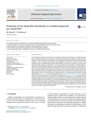
Prediction of the liquid film distribution in stratified-dispersed gas-liquid flow

Prediction of the liquid film distribution in stratified-dispersed
gas–liquid flow
M. Bonizzi n
, P. Andreussi
TEA Sistemi, Pisa, Italy
H I G H L I G H T S
A model for liquid film distribution in gas–liquid stratified dispersed flows has been derived.
The model allows the numerical calculation of the local axial liquid film height and velocity profiles.
Droplet deposition, gravitational drainage and wave spreading are relevant.
The strength of each mechanism depends on the underlying flow conditions.
The wave spreading affect is modelled as function of a modified Froude number.
a r t i c l e i n f o
Article history:
Received 30 July 2015
Received in revised form
28 October 2015
Accepted 9 November 2015
Available online 14 December 2015
Keywords:
Stratified dispersed gas–liquid flows
Liquid film distribution
Multiphase flow modelling
Entrainment
Deposition
Wave spreading
a b s t r a c t
A mathematical model for predicting the circumferential liquid film distribution in stratified-dispersed
flow is presented. Objective of the model is to describe the typical flow conditions of wet gas trans-
portation in long, near-horizontal pipelines. In these applications, depending on the gas velocity and pipe
diameter, a large asymmetry of the liquid film distribution may arise. The model is based on the
assumption that in stratified-dispersed flow, liquid droplets can only be entrained by the gas from the
thick liquid layer flowing at pipe bottom. It is also assumed that the deposition of smaller droplets is
related to an eddy diffusivity mechanism and regards the entire pipe circumference, while larger dro-
plets deposit by gravitational settling on the pipe bottom. These assumptions explain the formation of a
thin, non-atomizing film in the upper part of the pipe. The presence and flow structure of this film
appreciably affect the pressure gradient and the liquid hold-up in the pipe and are of great importance in
flow assurance studies. The model has been validated against i) the experimental observations recently
published by Pitton et al. (2014), the data collected by ii) Laurinat (1982), iii) Dallman (1978), and iv) the
predictions of three-dimensional CFD simulations conducted by Verdin et al. (2014). It is shown that the
relevant mechanisms which are responsible for the liquid film distribution are the gravitational film
drainage, droplet entrainment/deposition and wave spreading. In particular, at high gas velocities and/or
small pipe diameters, the asymmetry of the liquid film diminishes owing to the wetting mechanism of
wave spreading which makes the distribution of the film more uniform in the circumferential direction.
As the gas velocity diminishes and/or for larger pipe diameters, wave spreading is less effective and for
these flow conditions only gravitational drainage and droplet entrainment/deposition are responsible for
the more asymmetric shape of the liquid film.
2015 Elsevier Ltd. All rights reserved.
1. Introduction
Pipeline transportation over long distances of natural gas or
saturated steam in presence of a liquid phase is a common practice
in the oil and the geothermal industry and can be extremely
challenging when major flow assurance issues, such as corrosion
or solid formation and deposition on pipe wall arise. In near-
horizontal pipes, stratified flow conditions are encountered at
moderate phase velocities. At increasing the gas velocity, only part
of the liquid flows at the pipe wall, while the remaining liquid is
entrained by the gas in the form of droplets which tend to deposit
back onto the wall layer. The competing phenomena of droplet
entrainment and deposition determine the liquid hold-up in the
pipe and appreciably affect the pressure gradient. In large pipes
Contents lists available at ScienceDirect
journal homepage: www.elsevier.com/locate/ces
Chemical Engineering Science
http://dx.doi.org/10.1016/j.ces.2015.11.044
0009-2509/ 2015 Elsevier Ltd. All rights reserved.
n
Corresponding author. Tel.: +390506396140
E-mail address: marco.bonizzi@tea-group.com (M. Bonizzi).
Chemical Engineering Science 142 (2016) 165–179

the resulting flow pattern is usually classified as stratified-
dispersed flow, while in smaller pipes as horizontal annular flow.
The critical flow parameter to be measured in stratified-
dispersed flow is the flow rate and thickness distribution of the
liquid layer flowing at pipe wall. This is because the split of the
liquid phase determines the overall liquid hold-up in the pipe and
the value of the frictional pressure losses. Besides to the fluid-
dynamic issue, a better knowledge of the flow behavior of the wall
layer has many implications in flow assurance studies. In parti-
cular, the effectiveness of the inhibitors usually adopted to prevent
pipe corrosion depends on the formation of a liquid film around
the pipe wall.
In stratified-dispersed flow, the flow field presents strong 3-D
features. This makes difficult to describe this flow pattern in
transient 1-D flow simulators, such as the model proposed by
Bonizzi et al. (2009). In industrial applications, these simulators
are widely adopted for flow assurance studies, but often their
predictions are poor. The main objective of the present work is to
develop a detailed model of stratified-dispersed flow. This model
can then be coupled with a 1-D flow simulator and provide a
complete picture of this flow pattern.
Stratified-dispersed or horizontal annular flow is more com-
plicated than annular flow in a vertical pipe, due to the gravity
force, which typically causes an asymmetrical liquid film dis-
tribution around the pipe circumference. For instance, Paras and
Karabelas (1991) and Williams et al. (1996) observed significant
gradients of the liquid film height in the circumferential direction
and large vertical gradients of the droplet concentration. These
authors used a sampling probe to measure droplet concentration
and a conductance technique to measure the local film heights.
One of the pioneering investigations on horizontal annular flow
has been carried out by Butterworth (1969), who measured the
film thickness distribution of air/water flow in a 3.18 cm horizontal
pipe with a conductance method. This author argued that five
mechanisms may contribute to the asymmetrical film distribution:
Gravitational drainage.
Spreading of the film by wave motion.
Liquid transfer because of atomization and deposition effects.
Interfacial stresses due to the gas secondary flow.
Surface tension effects.
At the end of his analysis, Butterworth concluded that the film
thickness distribution was determined by a balance between the
film drainage due to gravitational effects and the upward liquid
movement associated with the lateral spreading of large
disturbance waves.
A similar investigation was carried out by Lin et al. (1985) who
analyzed the film distribution in a 2.69 cm I.D. pipe using a needle
probe approach and performed a modelling analysis based on the
fundamental conservation equations of mass and momentum
written for the liquid film. These authors suggest a relevant effect
of the term associated with the gas secondary flow.
Laurinat (1982) conducted an experimental study of air–water
horizontal annular flow in a 5.08 cm I.D. pipe. In these experi-
ments the liquid film height was measured at 7 different cir-
cumferential locations using conductivity probes. Laurinat et al.
(1985) developed a 2-D model of liquid flow based on momentum
conservation equations, where both normal and tangential stres-
ses were considered. These authors found that a good agreement
with the experimental data could be obtained by acting on the
normal shear stress along the circumferential coordinate, while in
their model the effect of gas secondary flow was negligible.
In both afore mentioned models, the direction of the gas sec-
ondary flows was modelled to be upwards, namely with flow
directed downward along the vertical pipe diameter and upward
at the walls. Nonetheless, it should be remarked that some con-
troversy exists on the role of secondary gas flows in horizontal
two-phase flows. For instance, Fisher and Pearce (1993) deter-
mined the liquid film distributions for horizontal annular flow in a
5 cm I.D. pipe and developed a model that neglected the second-
ary flow effect; yet they report a fair agreement between model
predictions and the corresponding experimental measurements.
Secondary flows have been extensively investigated in the lit-
erature, and contradictory findings were published. The first
detailed observations of turbulent secondary flows were made by
Nikuradse (1930) and Prandtl (1927). The first used both flow
visualization with a red dye and Pitot tube measurements to map
the gas velocity profiles. The second suggested that the shape of
the measured velocity contours implied the existence of secondary
motion. According to Prandtl, turbulent velocity fluctuations exist
tangent to the curved contours of constant mean axial velocity (i.e.
isotach) surfaces, and these fluctuations increase with increased
curvature of the isotachs. Hence, the resulting Reynolds stresses
will generate forces on the convex side of the isotachs, which give
rise to the secondary flows. According to this observation, con-
sidering the case of a gas–liquid flow in a circular pipe, a cir-
cumferential disturbance such as the asymmetric distribution of
the liquid film (which would then lead to an asymmetrical inter-
facial roughness) might be sufficient in order to get secondary
flows initiated under turbulent gas flow conditions.
As mentioned above, in a circular duct the gas secondary flow
may be directed downwards along the vertical diameter or
upwards. Darling and McManus (1969) conducted an experiment
using a pipe with an eccentric thread, being deeper at the bottom
than the top. In this way they could simulate the conditions of a
non-uniform liquid film. Using hot-wire velocity measurements,
they found that the gas velocity profile was skewed toward the
bottom of the pipe. This indicates the presence of secondary flows
directed downwards along the vertical diameter.
Similar observations were reported by Andreussi and Persen
(1987) and by Vlachos et al. (2003). The latter authors adopted a
Laser Doppler method to measure the time-averaged gas flow field
in 5 cm and 2.4 cm pipes for gas–liquid stratified flow and con-
firmed the presence of secondary flows, directed downwards
along the vertical diameter. It has to be remarked that the range of
gas superficial velocities investigated by Vlachos et al. (2003) was
below 12 m/s.
Dykhno et al. (1994) took detailed velocity measurements in
air–water stratified/annular horizontal flows for a 9.5 cm pipe.
Using Prandtl's interpretation of curved isotachs, they confirmed
the existence of secondary flows. These authors were the first to
identify conditions under which the direction of the secondary
flows changed: while at lower gas velocities (typically o20 m/s)
the motion of secondary flows was directed downward at the
center, at higher gas velocities the secondary flows appeared to be
directed upwards. Dykhno et al. (1994) argued that the atomiza-
tion of the liquid film was responsible for the change in direction
of the gas secondary flows.
Dallman (1978) investigated air–water annular flows in a
2.3 cm inner diameter pipe, and, from his measurements of local
liquid film thickness, proposed to correlate the film height with a
modified Martinelli flow parameter. Hurlburt and Newell (1997)
proposed a simplified model for estimating the liquid film dis-
tribution, based on the Laurinat et al. (1985) derivation. These
authors analyzed available experimental measurements of the
liquid film heights for gas–liquid stratified/dispersed flows gath-
ered by different researchers for horizontal pipes, and proposed a
correlation for predicting the degree of asymmetry of the liquid
film, based on a modified Froude number, which represents the
square root of the ratio between the gas kinetic energy and the
work required to pump the liquid from the bottom to the top of
M. Bonizzi, P. Andreussi / Chemical Engineering Science 142 (2016) 165–179166

the pipe. Hurlburt and Newell (1997) succeeded in eliminating the
large scatter in the data plotting the ratio of the average liquid film
height to liquid film height at the pipe bottom versus the modified
Froude number defined as aforementioned. Moreover, the authors
made model assumptions which further simplified the mathe-
matical liquid film model envisaged by Laurinat et al. (1985); in
particular the term associated to the gas secondary flows was
altogether dropped from model equations. Nonetheless Hurlburt
and Newell (1997) found good agreement with the experimental
data, despite having to tune a coefficient which altered the mag-
nitude of the normal shear stress term associated to the wave
spreading effect. These authors concluded that the two relevant
mechanisms driving the distribution of the liquid film around the
pipe walls are the turbulent normal shear stresses in the cir-
cumferential direction (which is related to the wave spreading)
and the drainage of the liquid film from the top of the tube due to
gravity.
During the latest years, some interesting work, conducted
using three-dimensional Computational Fluid Dynamics (i.e. CFD)
packages, has been published in the literature. McCaslin and
Desjardins (2014) simulated three-dimensional liquid–gas annular
flows using CFD methods, and, by applying dimensional analysis,
these authors selected the relevant governing parameters of the
multi-phase flow problem under investigation. From the obtained
CFD results, McCaslin and Desjardins (2014) showed that, for the
cases in which the liquid is not significantly drained (in other
words when the asymmetry of the liquid film distribution is not
too pronounced and the gradient of the liquid film height along
the circumferential coordinate is not particularly high), the action
of the surface waves tends to drive the liquid up the pipe walls. By
reducing the magnitude of the gas stream kinetic energy, the CFD
results indicated more significant asymmetry of the liquid film
distribution. Quite interestingly, under these conditions, McCaslin
and Desjardins (2014) noticed an almost total absence of the
upwards liquid film motion by wave spreading.
Verdin et al. (2014) conducted CFD studies for large diameter
pipes (3800
inner diameter), and their main finding was that a very
significant asymmetry of the liquid film distribution resulted,
which became far more evident as the gas velocity diminished.
These authors found that almost all the continuous liquid phase
(which the authors called the liquid pool) was sitting in the bot-
tom part of the tube, and a very thin liquid film (with a thickness
never greater than 300 μm at the top of the pipe) draining from
the top of the tube. These authors concluded that droplet
deposition was the physical mechanisms responsible for sustain-
ing the thin liquid film draining along the inner perimeter.
In a recent paper, Pitton et al. (2014) report an experimental
investigation of stratified-dispersed flow in a horizontal pipe,
7.9 cm I.D. diameter operating under an appreciable pressure.
These authors measured the circumferential liquid film distribu-
tion with an array of conductance probes, which were also used to
measure the liquid entrainment and the rates of droplet entrain-
ment and deposition by the tracer method, originally developed
by Quandt (1965) to study vertical annular flows. The main results
of this investigation have been a fairly accurate measurement of
the liquid entrainment and a good estimate of the rate of droplet
entrainment, which has been found to be one order of magnitude
larger than the values usually adopted in 1-D simulation tools and
of the values determined in vertical annular flow.
The experimental observations of tracer mixing along the pipe,
led Pitton et al. (2014) to conclude that a simple two-field model
for describing the underlying physics within a one-dimensional
modelling framework was not feasible. They suggested to model
the flow structure using a three-field model, whereby the liquid
phase is split between a continuous liquid film flowing at pipe wall
and two distinct droplet fields: smaller droplets able to interact
with gas turbulent motions (and eventually with the gas second-
ary flow) and larger droplets which move on a trajectory flight and
re-deposit on the pipe bottom by gravitational settling. In vertical
annular flows, the simultaneous presence of two different
mechanisms of droplet transfer (eddy diffusion and trajectory
motion) was reported by Andreussi and Azzopardi (1983).
Another interesting observation reported by Pitton et al. (2014)
is that the liquid film tends to be wavy only for angles up to about
70° from the bottom for a significant range of flow parameters. The
remaining part of the wall layer appears to be smooth, with the
total absence of a large disturbance waves. This result can be
coupled with the experimental and theoretical work by Andreussi
et al. (1985), who found that the critical film flow rate for the
initiation of large waves closely corresponds to the film flow rate
below which no entrainment occurs. One may then conclude that
the atomization process would only be relevant for the bulk of the
liquid film sitting at the pipe bottom, whereas the thinner liquid
film wetting the remaining part of the pipe wall would only be
characterized by the two phenomena: the deposition of smaller
droplets and the subsequent drainage of the deposited liquid from
the top to the bottom of the pipe.
The experimental work reported by Pitton et al. (2014) did not
include direct measurements of the gas secondary flow, but,
according to these authors, the tracer distribution in the wall layer
appears to be more consistent with the assumption of a weak gas
secondary motion directed downwards along the pipe walls rather
than upwards. In what follows a unified laminar-turbulent two-
dimensional model of liquid flow in horizontal stratified-dispersed
flow is presented and it is shown that this model provides a fairly
good fit to the experimental measurements of Pitton et al. (2014).
For these data, the main mechanism which is able to counteract
the drainage of the liquid film appears to be the droplet deposi-
tion. It is also shown that the normal shear stress gradient due to
the velocity fluctuations of the liquid layer in the circumferential
direction (term associated to the wave spreading effect) can be
relevant at large gas velocities and/or small pipe diameters, such
as the flow conditions investigated by Dallman (1978) and Laurinat
(1982).
2. Model derivation
The mathematical model developed in the present work is a
modified version of that proposed by Laurinat et al. (1985). With
reference to Fig. 1, let θ denote the angle measured from the
bottom of the pipe, R the pipe radius, x, y and z the circumferential,
Fig. 1. Adopted frame of reference for model development.
M. Bonizzi, P. Andreussi / Chemical Engineering Science 142 (2016) 165–179 167

radial and axial coordinates respectively. Eqs. (52)–(54) of the
Laurinat et al. (1985) work represent the momentum equation
written in the axial coordinate, circumferential coordinate, and the
conservation of mass respectively:
I1τþ
yz;h þ
I2
Rþ
∂τþ
xz
∂θ
¼ Γþ
z ð1Þ
I1τþ
yx;h þ
I2
Rþ
∂τþ
xx
∂θ
À
I2
Rþ
Fr
sin θþ
cos θ
Rþ
dh
þ
dθ
!
¼ Γþ
x ð2Þ
dΓþ
x
Rþ
dθ
¼ Rþ
D ÀRþ
A ð3Þ
The derivation of these equations is reported in Appendix A.
These equations are written in non-dimensional form and the
superscript þ
represents the corresponding quantity made non-
dimensional. In particular, the shear stresses are normalized with
respect to the gas-wall shear stress:
τG ¼
1
2
f GsρGu2
G ð4Þ
In the equation above the gas-wall shear stress is computed
using the standard Fanning correlation for turbulent flow in a
smooth pipe (f Gs ¼ 0:046ReÀ 0:2
Gs ). The τþ
yz;h
term is the ratio of the
interfacial shear stress to the gas wall shear stress:
τþ
yz;h ¼
τyz;h
τG
¼
f int
f Gs
ð5Þ
The term τþ
yx;h
in Eq. (2) denotes the shear stress exerted by the
gas secondary flow on the liquid film.
Eq. (4) allows to introduce the friction velocity uÃ
,
uÃ
¼
ffiffiffiffiffi
τG
ρL
r
ð6Þ
The non-dimensional liquid film height and the pipe radius are
then defined as:
h
þ
¼
huÃ
υL
; Rþ
¼
RuÃ
υL
ð7Þ
and the Froude number as:
Fr ¼
τG
ρLgR
ð8Þ
The terms on the right hand side of Eqs. (1) and (2), Γþ
z and
Γþ
x , denote the non-dimensional axial mass flow rate per unit
circumferential length and the circumferential mass flow rate per
axial unit length, respectively:
Γþ
z ¼
Γz
μL
¼
Z h
þ
0
uþ
z dyþ
¼ uþ
z

h
þ
ð9Þ
Γþ
x ¼
Γx
μL
¼
Z h
þ
0
uþ
x dyþ
¼ uþ
x

h
þ
ð10Þ
As shown above, the mass flow rates per unit length are made
non-dimensional with respect to the liquid dynamic viscosity μL.
As usual, the average value of a variable in the radial direction is
defined as:
φ

¼
Rh þ
0 φdyþ
h
þ ð11Þ
The terms on the right hand side of Eq. (3) denote the non-
dimensional droplets deposition and atomization fluxes
(kg= m2
s
À Á
):
Rþ
D ¼ RD
1
ρLuÃ
ð12Þ
and
Rþ
A ¼ RA
1
ρLuÃ
ð13Þ
respectively. Provided that adequate closure laws are found for the
shear stress terms (τþ
yz;h
; τþ
xz ; τþ
yx;h
; τþ
xx ), and likewise for the
deposition and atomization fluxes, Eqs. (1)–(3) represent a system
of 3 equations in 3 variables (Γþ
z ; Γþ
x ; h
þ
).
The model developed by Andreussi et al. (1985) to predict the
liquid film flow rate at the onset of the large disturbance wave
regime can be used to calculate the critical mass flow rate, below
which atomization of the liquid film shall not occur:
Γz;c ¼
μL
4
Rez;c; ð14Þ
where the critical liquid Reynolds number can be computed as:
Rez;c ¼ 4
Γz;c
μL
¼ 7:3 log 10ω
À Á3
þ4:22 log 10ω
À Á2
À263 log 10ω
À Á
þ439
ð15Þ
In this correlation, the dimensionless group ω ¼ μL=μG
À Á
ffiffiffiffiffiffiffiffiffiffiffiffiffi
ρG=ρL
p
was indicated by Andreussi et al. (1985) as the only
quantity upon which the critical liquid Reynolds number depends.
As stated by Pan and Hanratty (2002), measurements in hor-
izontal flows by Laurinat (1982) indicate that the critical Reynolds
number is around 480, or in other terms
Γz;c ¼ 120μL ð16Þ
Under conditions where
Γz ¼ ρL uzh ih
À Á
oΓz;c ¼ 120μL ð17Þ
atomization of the liquid film shall not occur and the equations
which express the mass and momentum conservation along the
circumferential direction can be simplified as follows:
dΓx
Rdφ
¼ RD φ
À Á
ð18Þ
and
μL
∂2
ux
∂y2
¼ ρLg sin φ ð19Þ
Eqs. (18) and (19) are written in dimensional form, the angle φ
is taken from the top of the tube (φ ¼ πÀθ), and the Dirichlet and
Neumann boundary conditions related to the x-momentum Eq.
(19) are as follows:
ux;y ¼ 0 ¼ 0;
∂ux
∂y y ¼ h ¼ 0

ð20Þ
Eq. (19) is the typical laminar film motion equation and can be
easily integrated taking into account the boundary conditions
expressed in Eq. (20). This allows the circumferential velocity
variation to be determined as function of the radial coordinate:
ux y; φ
À Á
¼
ρLg
μL
y2
2
ÀhðφÞy

sin φ ð21Þ
Eq. (21) can then be used to compute the circumferential mass
flow rate per unit axial length:
Γx φ
À Á
¼
Z y ¼ h φð Þ
0
ρLux y; φ
À Á
dy ¼ À
ρ2
L gh φ
À Á3
sin φ
3μL
ð22Þ
If the circumferential mass flow rate per unit axial length is
known at the given angle, Eq. (22) allows the liquid film height to
be determined as
h φ
À Á
¼
ffiffiffiffiffiffiffiffiffiffiffiffiffiffiffiffiffiffiffiffiffiffiffiffiffi
3μL jΓxðφÞj
ρ2
L g sin φ
3
s
ð23Þ

3. Closure equations
The system of Eqs. (1)–(3) requires empirical closures for the
shear stresses and the fluxes of droplets deposition and entrain-
ment. The first term requiring closure is that related to the inter-
facial gas–liquid shear stress τþ
yz;h
. When the liquid film is turbu-
lent, following the recommendations of Laurinat (1982), the shear
stress is assumed to be given by the equation
τþ
yz;h ¼
τyz;h
τG
¼
f int
f Gs
¼ C3 þC4Γþ
z ð24Þ
where, according to Laurinat (1982), C3 % 2 and C4 % 10À 3
. Under
a laminar liquid flow regime (i.e. when Eq. (17) is satisfied), the
equation recommended by Andreussi et al. (1985) can be adopted,
τþ
yz;h ¼
τyz;h
τG
¼
f int
f Gs
¼ 1þ0:023 h
þ
G À10:9
À Á
ð25Þ
where h
þ
G ¼
huÃ
G
νG
, uÃ
G ¼
ffiffiffiffiffiffiffi
τyz;h
ρG
q
.
The equation used to predict τþ
yx;h
is based on the experiments
of Darling and McManus (1969), who measured the film roughness
distribution for a horizontal air–water annular flow in an eccen-
trically threaded pipe. The following correlation has been derived
from the analysis of their measurements:
τþ
yx;h ¼
τyx;h
τG
¼ C5τI sin θ ð26Þ
In Eq. (26) τI denotes the (non-dimensional) average interfacial
shear stress between the gas core and the liquid film, while the
constant C5 % 3:0 Â 10À2
.
The normal shear stress in the circumferential direction is
assumed to be characterized by flow oscillations (in the x-direc-
tion) taken as angular deviations of the main flow (in the axial
direction), and therefore to scale with the square of the local mean
axial velocity:
τþ
xx ¼
τxx
τG
¼ ÀC1uþ
z 2 ¼ ÀC1
Γþ
z
h
þ
!2
ð27Þ
Eq. (27) is similar to the representation of the wave-spreading
effect proposed by Butterworth (1969). According to this author,
the wave spreading mechanism is based on the assumption that
large disturbance waves drive the liquid film in front of each wave
up the tube walls. In their model, Laurinat et al. (1985) tuned the
coefficient C1 in order to fit the experimental data. The value
adopted for this term (C1 ¼ O 10À 1

) makes the normal shear
stress to be the main term able to balance the gravitational forces
acting on the liquid film, and the authors speculated that the
mechanisms associated to entrainment and deposition were of
secondary order.
The present model shows that the competing physical
mechanisms which affect the resulting liquid film distribution are
a balance between gravitational drainage, droplet deposition and
wave spreading. The dominant terms are problem dependent. In
fact the C1 coefficient needs an adequate tuning in order to match
the measured data with fair accuracy. It will be shown that,
depending on the specific flow conditions under investigation, the
wave spreading effect might be altogether dropped from the
model equations. Moreover, in the Section 6, where the model
results are compared against the data collected by Dallman (1978)
and Laurinat (1982), a novel correlation for estimating the mag-
nitude of the C1 coefficient is proposed.
The last term requiring a closure is the dispersion of the z-
momentum in the x-direction, which is modelled following the
recommendations by Townsend (1970):
τþ
xz ¼
τxz
τG
¼ C2
duþ 2
z
dθ
ð28Þ
In the above equation the constant has an order of magnitude
around C2 % 10À 2
. If Eqs. (24)–(28) are inserted into Eqs. (1) and
(2), the momentum equations in the z and x direction can be
written as follows:
I1τþ
yz;h þ
C2
Rþ I2
d
2
uþ
z 2
dθ2
¼ Γþ
z ð29Þ
I1C5τI sin θÀ
I2
Rþ C1
duþ 2
z
dθ
À
I2
Rþ
Fr
sin θþ
cos θ
Rþ
dh
þ
dθ
!
¼ Γþ
x ð30Þ
When the liquid film is turbulent, Eq. (30) can be greatly sim-
plified if the derivative of the axial velocity squared is expressed as
function of gradients along the circumferential direction of the
axial mass flow rate Γþ
z and the film height h
þ
:
duþ2
z
dθ
¼
d
dθ
Γþ
z
h
þ
!2
¼
2Γþ
z
h
þ 2
dΓþ
z
dθ
À
Γþ
z
h
þ
dh
þ
dθ
#
ð31Þ
Eqs. (29) and (24) can then be deployed in order to derive a
relation between the angular gradients of the axial mass flow rate
and that of the liquid film height:
dΓþ
z
dθ
¼ φ
dh
þ
dθ
ð32Þ
If Eqs. (32) and (31) are inserted into Eq. (30), an equation for
the circumferential gradient of the liquid film height is immedi-
ately derived:
dh
þ
dθ
¼
Γþ
x ÀI1C5τI sin θþ I2
Rþ
Fr
sin θ
I2
Rþ
2C1Γþ
z
hþ 2
Γþ
z
h þ Àϕ

À cos θ
R þ
Fr
h i ð33Þ
Under turbulent flow conditions of the liquid film, the system
that will be numerically solved is therefore composed by Eqs. (33),
(29) and (3).
In order to close the system, the fluxes of droplets atomization
and deposition must be defined. The atomization flux is based on
the recommendation by Williams et al. (1996) and Pan and Han-
ratty (2002):
RA ¼
kAu2
G ρGρL
À Á1=2
σGL
ΓZ ÀΓZ;C
À Á
ð34Þ
The atomization constant in Eq. (34) has been taken to be
kA % 2:0 Â 10À 6
. This value is directly derived from the experi-
ments of Pitton et al. (2014) and is about one order of magnitude
larger than the value adopted by Laurinat et al. (1985) and in the
1-D transient models used for flow assurance studies.
The flux of droplet deposition is usually expressed as:
RDh i ¼ kDCB ð35Þ
where kD denotes the deposition velocity and CB the bulk con-
centration (as mass of liquid droplets per unit volume):
CB ¼
EWL
QGS
¼ ρL
αD
αG
ð36Þ
In the above equation E denotes the entrainment ratio (i.e. ratio
of the mass flow carried by the liquid droplets to the overall liquid
mass flow rate), WL is the total liquid mass flow in the pipe, QG the
gas volumetric flow rate, S the slip ratio between the liquid dro-
plets and the gas core velocity, αD the liquid droplets volume
fraction and αG the gas volume fraction. Eq. (35) denotes an
average over the pipe cross section; the local deposition can be
expressed assuming a concentration profiles of the droplets which

can be derived as proposed by Paras and Karabelas (1991):
C Yð Þ ¼ C0exp À
uT
ϵ
Y

ð37Þ
In the above equation C0 denotes the droplets concentration at
the bottom of the pipe, uT is the droplet settling velocity, ε the
turbulent diffusivity of the droplets, and Y the vertical distance
from the bottom pipe (Y ¼ R 1À cos θ
À Á
). The following equation
arises for the local droplet deposition flux:
RD θ
À Á
¼ kD θ
À Á
C0exp Àkð Þexp ðk cos θÞ ð38Þ
where k ¼ uT R
ε

. The averaged droplets deposition flux RDh i is
given by the following integral of the local deposition value:
〈RD〉 ¼
R π
0 RD θ
À Á
dθ
π
ð39Þ
The deposition velocity can be computed as a blending
between two different deposition mechanisms: the gravitational
and turbulent droplet settling. As illustrated by Pan and Hanratty
(2002), the gravitational droplet deposition can be expressed as
follows:
kD;g θ
À Á
¼
1
13:5
ρLgd
1:6
ρG
0:4μG
0:6
#5=7
cos θ ð40Þ
Assuming a Gaussian distribution for the radial turbulent
velocity fluctuations, the turbulent deposition coefficient can be
computed as:
kD;t ¼
0:9
ffiffiffiffiffiffiffiffiffi
14π
p uG
ffiffiffiffiffiffiffiffiffiffi
f int;D
2
s
ð41Þ
In the above equation f int;D is the interfacial friction factor
relation proposed by Dallman et al. (1979) for horizontal gas–
liquid separated flows. The concentration at the pipe bottom, C0
can be obtained from the cross-sectional area average:
C0 ¼
π
2
CBexp kð Þ
R π
0 sin θ
À Á2
exp k cos θ
À Áh i
dθ
ð42Þ
Under flow conditions such that Eq. (17) is satisfied, Eq. (18) can
used to calculate the angular mass flow rate per axial unit length
by integrating the local deposition flux expressed from Eq. (38):
Γx φ
À Á
¼ RkD;tC0exp Àkð Þ
Z φ
0
exp Àk cos ϑ
À Á
dϑ ð43Þ
The transcendent integral in Eq. (43) can be numerically solved
using the appropriate Taylor expansion of the integrand function.
It has to be remarked that, for the portion of the liquid film dis-
tribution that does not experience atomization, the turbulent
deposition velocity is deployed in Eq. (43).
Once the circumferential mass flow rate per axial unit length is
known, the film thickness immediately follows from Eq. (23).
Table 1 indicates the equations employed by the model in the two
distinct regions which characterize the liquid film distribution
profile.
4. Numerical model
The system of equations illustrated in the earlier sections
represents an elliptic set of equations that can be solved provided
that the appropriate boundary conditions are supplied. The
equations will be integrated along half the circumference peri-
meter (i.e. for θA 0; π½ Š). Therefore the first boundary conditions to
take into consideration is the symmetry condition on the cir-
cumferential mass flow rate per unit axial length:
Γx 0ð Þ ¼ Γx πð Þ ¼ 0 ð44Þ
Inspection of Eq. (30) provides the constraints required to
satisfy the symmetry condition expressed by Eq. (44) above:
dh
þ
dθ

θ ¼ 0
¼
dh
þ
dθ

θ ¼ π
¼ 0 ð45Þ
duþ2
z
dθ

θ ¼ 0
¼
duþ 2
z
dθ

θ ¼ π
¼ 0 ð46Þ
Besides the conditions above, the system of equations can be
integrated if the appropriate Dirichlet boundary condition is pre-
scribed at one solution boundary, i.e. h θ ¼ 0 ¼ h 0ð Þ

.
The equations have been numerically integrated adopting a
first-order Runge–Kutta (i.e. Euler's method) discretization
scheme:
dy
dx
¼ Φ x; yð Þ )
yjþ 1 Àyj
xjþ 1 Àxj
¼ Φ xj; yj

ð47Þ
Within the numerical solution scheme, Eq. (17) is checked for
each numerical point of the angular grid. When the equation is
satisfied, in order to guarantee a smooth transition from the tur-
bulent (i.e. Γz 4Γz;c) to the laminar (i.e. Γz rΓz;c) liquid film
region, Eq. (43) is employed in order to back-calculate the turbu-
lent deposition velocity as follows:
Γx;t θtr
À Á
¼ Γx;l πÀθtr
À Á
ð48Þ
In Eq. (48) the subscripts t and l denote turbulent and laminar
flow regime conditions for the liquid film, and θtr denotes the
angle at which transition occurs (i.e. the angular node for which
Eq. (17) is satisfied). Equation Γx;t θtr
À Á
is calculated from the
numerical integration of Eq. (3), while the Γx;lam πÀθtr
À Á
term
comes from solution of Eq. (43). One then derives the following
expression for the kD;t deposition coefficient:
kD;t ¼
Γx;turb θtr
À Á
RC0exp Àkð Þ
R π À θtr
0 exp Àk cos φ
À Á
dφ
ð49Þ
Other details related to the adopted numerical scheme can be
found in Appendix B.
5. Model validation
The experimental data by Pitton et al. (2014) relate to gas–
liquid annular flow in a horizontal pipe having a 7.8 cm inner
diameter, an outlet pressure set around 5 bar, and liquid and gas
superficial velocities of 0.068 and 25.5 m/s, respectively. Table 2
below summarizes the relevant experimental measurements.
In this Table, αLF denotes the film liquid hold-up, ΦA the film
atomization rate, ΦB the droplets deposition rate at the bottom of
the pipe, ΦR the mass flow rate of the non-atomizing film flowing
in the upper part of the pipe and E the entrainment ratio. The
liquid film holdup, knowing the circumferential distribution of the
Table 1
Adopted equations by liquid film model.
Γz 4Γz;c Mass
equation
x-Momentum z-Momentum τþ
yz;h
dimensionless
Â Ã
True (atomiz-
ing film)
Eq. (3) Eq. (33) Eq. (29) Eq. (24)
False (only
deposition)
Eq. (43) Eq. (23) Eq. (29) Eq. (25)

film, can be calculated by the following integral:
αLF ¼
R π
0 DÀh θ
À ÁÀ Á
h θ
À Á
dθ
πR2
ð50Þ
The liquid film flow rate is related to the local axial flow rate
per circumferential length as follows:
WLF ¼ 1ÀEð ÞWL ¼ 2
Z π
0
Γz θ
À Á
Rdθ ð51Þ
The average axial film flow rate per unit length can be found by
the following averaging:
ΓLF ¼ 〈Γz〉 ¼
R π
0 Γz θ
À Á
dθ
π
ð52Þ
Eqs. (51) and (52) give
WLF ¼ πD Γz

¼ πDΓLF ð53Þ
The rates of deposition/entrainment given by Table 2 above are
linked by the following identity:
ΦA ¼ ΦD ¼ ΦB þΦR ð54Þ
The drainage rate of the non-atomizing film corresponds to the
rate of deposition of the smaller droplets which are carried by the
gas core in the upper part of the pipe tube. The relation between
the entrainment/deposition rate and flux is defined by the fol-
lowing equation:
Φq ¼ Rq
P
A
ð55Þ
In the above equation P and A denote the pipe perimeter and
cross section area respectively. For circular tubes P
A ¼ 4
D, D being the
pipe diameter. If we apply Eq. (55) to the droplet deposition rate,
and use the deposition flux which obeys Eq. (35), we can then
write the following equation:
ΦD ¼
4
D
kDCB ð56Þ
According to the data analysis performed by Pitton et al. (2014),
the deposition rate is composed by two terms which arise from
different physical mechanisms: the deposition rate ΦB due to the
gravitational settling of the larger droplets, and the deposition rate
ΦR on the upper pipe wall which is followed by the film drainage
from the top to the bottom of the pipe. The deposition velocity
kD;g, given by Eq. (40), characterizes the deposition coefficient for
the process occurring at the pipe bottom, whereas the velocity kD;t,
as given by Eq. (41), is responsible for the deposition of the dro-
plets which subsequently form the draining liquid film. Eq. (40)
involves a reference droplet diameter which can be predicted with
the equation proposed by Pan and Hanratty (2002):
d $
3:6
0:765
ffiffiffiffiffiffiffiffiffiffiffiffiffiffiffiffiffiffiffiffiffiffiffiffiffiffi
0:0091σGLD
ρGu2
G
s
ð57Þ
Eqs. (40) and (41) allow the calculation of the reference
deposition coefficients:
kD;g $ 1:4
m
s
h i
ð58Þ
kD;t $ 0:2
m
s
h i
ð59Þ
Let β denote the angle around the pipe perimeter which
encloses the base film (i.e. the portion of the liquid film which
undergoes the atomization process and therefore characterized by
a turbulent regime), then an averaged value for the deposition
coefficient can be estimated as follows:
kD $
βkD;g þ πÀβ
À Á
kD;t
π
ð60Þ
Pitton et al. (2014) report that the β angle is around 70°; from
Eq. (60) kD $ 0:7 m
s
Â Ã
is calculated. From Eq. (56) the bulk liquid
droplet concentration can be then estimated,
CB ¼
D
4
ΦD
kD
$ 1:9
kg
m3
!
ð61Þ
Eq. (42), which expresses the relation between the bulk and
bottom liquid droplets concentration, can be numerically solved
and the concentration of the liquid droplets at the bottom is found
to be C0 $ 9:3 kg
m3
h i
. From the experimental data, assuming a C3
coefficient (see Eq. (24)) of 2.0, we can determine the C4 coeffi-
cient from the experimental measurement of the pressure gra-
dient. The momentum equation in the z-direction, assuming
steady-state conditions can be written as:
À 1ÀαLFð Þ
dP
dz
À
τI
R2
DÀ2 h
À Á
¼ 0 ð62Þ
The average liquid height is related to the average liquid film
holdup by the following equation:
〈h〉 ¼
R π
0 h θ
À Á
dθ
π
¼
D
2
1À
ffiffiffiffiffiffiffiffiffiffiffiffiffiffiffi
1ÀαLF
p
ð63Þ
For the specific problems under examination we find that h

¼ 409 μm
Â Ã
and τI Š: Using Eq. (4) for calculating the gas shear
stress and Eq. (53) for computing the averaged axial mass flow rate
per unit circumferential length, leads to the calculation of
C4 ¼ 1:27 Â 10À3
. Table 3 below reports the values of C1 and C2
used in the present model in order to attain the best agreement
with the measured data. While the C2 coefficient, proportional to
the diffusion of the axial momentum in the circumferential
direction τþ
xz , is set at a value which has the same order of mag-
nitude as that deployed by Laurinat et al. (1985) (the values taken
are C2 ¼ 1:0 Â 10À2
in the current model and C2 ¼ 1:7 Â 10À2
in
the Laurinat et al. (1985) work), it should be remarked that the C1
coefficient, related to the wave spreading term τþ
xx as expressed by
Eq. (27), was taken two order of magnitudes smaller than the
values (around O 10À 1

) typically assumed by Laurinat et al.
(1985). In fact larger values led to erroneous model results,
whereas smaller values led to numerical instability issues. At this
stage, the gas secondary flows are not taken into consideration
(C5 ¼ 0).
In Fig. 2 The resulting liquid film profile is compared with the
experimental measurements.
Table 2
experimental data-set related to problem under investigation.
WL
kg
s
h i
WG
kg
s
h i
αLF ½ÀŠ h 0ð Þ½mmŠ dP
dz Pa
m½ Š ΦA
kg
m3 s
h i
ΦB
kg
m3 s
h i
ΦR
kg
m3 s
h i
E [dimensionless]
0.33 0.73 0.021 2.1 -940 68 60 8 0.47
Table 3
Coefficients used for closing the shear-stress model.
C1 τþ
xx
Â Ã
C2 τþ
xz
Â Ã
C3 τþ
yz;h
h i
C4 τþ
yz;h
h i
5:0 Â 10À 3
1:0 Â 10À 2 2:0 1:27 Â 10À 3

This figure indicates a fair agreement between the model pre-
dictions and the measurements. It should be remarked that the
clear inflection point at 35° is due to the discontinuity of the eddy
diffusivity model between the fully turbulent and the transition
regions, as explained in Appendix A. From the data collected by
the model, it is possible to numerically solve the integrals of Eqs.
(50) and (51), which allow to determine the liquid film holdup and
overall liquid film mass flow rate respectively. Table 4 shows the
comparison between the experimental measurements and the
numbers obtained from the model results. Fig. 3 shows the
cumulative liquid holdup (Eq. (50) is integrated in discrete steps
from the pipe bottom to the pipe top) associated to the liquid film
and the local axial velocity. From this graph one can appreciate
how the bulk of the liquid film is carried by the portion of the film
sitting at the pipe bottom.
It is interesting to notice that, for the problem under examination,
transition from the atomizing to the non-atomizing liquid film (cor-
responding to the threshold dictated by Eq. (17)) occurs for an angle
around θtr $ 961, which is larger than the experimentally determined
θtr $ 701. This information is readily extracted from the output of the
developed model in that, once the numerical model converges, for
each angular numerical cell, the value of the local axial mass flow rate
per circumferential unit length is known and the angle of transition
from turbulent to laminar liquid film regime is determined from
inspection of Eq. (17).
In order to evaluate the potential effects of gas secondary flows,
two opposite values for the constant C5 were taken
(C5 ¼ 73:0 Â 10À2
). It has to be remarked that the absolute
magnitude of C5 is consistent with the values suggested by Darling
and McManus (1969). A positive sign, in accordance with the
considered frame of reference, would imply secondary flows with
upward direction (up the wall and down the vertical center line); a
negative sign would instead dictate that the secondary flows are
modelled having a downward direction (down the walls and up
along the vertical center line).
The model results with inclusion of the τþ
yx;h
shear stress, with
opposite direction, are illustrated in Fig. 4, where, for sake of clarity,
also the results obtained neglecting the secondary flows are shown.
As shown in this figure, the effects of gas secondary flows are limited.
The most interesting result is related to the newly determined angle
θtr, at which transition to a non-atomizing liquid film takes place in
accordance with Eq. (17). In fact, while for the case of a positive
coefficient C5, the transition is predicted to occur at an angle
θtr $ 1021, for the case with negative coefficient C5, the transition is
predicted to occur at smaller angles (θtr $ 711), which is in excellent
agreement with the experimental observations. Other effects of the
adopted closure for the τþ
yx;h
on some relevant flow variables are
shown in Table 4 above.
Fig. 2. Resulting liquid film profile from the model and comparison with experi-
mental data points.
Table 4
model predictions for relevant flow variables.
C5 τþ
yx;h
h i
θtr [°] αLF ½ÀŠ WLF
kg
s
h i
E [dimensionless] ΦA
kg
m3 s
h i
ΦB
kg
m3 s
h i
ΦR
kg
m3 s
h i
0 96 0.022 0.197 0.4 56 50 6
þ3:0 Â 10À 2 102 0.023 0.211 0.35 60 54 6
À3:0 Â 10À 2 71 0.020 0.179 0.45 52 45 7
Fig. 3. Local axial velocity and cumulative liquid film holdup as predicted by the
model without secondary flows.
Fig. 4. Resulting liquid film profile from the model with or without the shear stress
accounting for the gas secondary flows and comparison with experimental data
points.

6. Discussion
The current model is based on the assumption that the liquid
film distribution around the pipe walls entirely depends on the
local liquid film regime, either laminar or turbulent. Hence, the
governing equations are chosen, as illustrated in Table 1, after the
axial film flow rate per unit circumferential length is determined
by Eq. (17). Under fully turbulent liquid film conditions (Γz 4Γz;c),
the model coincides with that proposed by Laurinat et al. (1985)
while it deviates from it under laminar liquid film flow conditions,
in that, as far as the governing equations along the circumferential
coordinate are concerned, only the deposition flux is accounted for
in the mass conservation equation, and the Navier–Stokes equa-
tions written for a laminar film apply for the conservation of
momentum. The assumptions made under laminar liquid film flow
conditions allow the immediate calculation (once the deposition
law has been determined) of the Γx term (Eq. (43)), from which
the local liquid film height follows from Eq. (23). Another impor-
tant difference is that, under fully laminar liquid film flow, the
normal shear stress term τþ
xx associated to the disturbance wave
spreading effect is taken to be absent from the model equations.
Objective of the current section is to validate the proposed model
against additional data, taken from the experimental work of
Dallman (1978), Laurinat (1982), and the three-dimensional CFD
investigation carried out by Verdin et al. (2014).
Table 5 summarizes the flow conditions for the selected test
cases taken from Laurinat (1982) and Dallman (1978).
In order to deploy the proposed model, the droplets con-
centration at the pipe bottom C0 must be estimated, as such
parameter is explicitly required by the droplets deposition flux
expressed in Eq. (38). Assuming that the droplet concentration law
coefficient k (i.e. C Yð Þ ¼ C0exp ÀkY=R
À Á
) has been computed, the C0
parameter is evaluated using Eq. (36) (which provides the relation
between the averaged droplets concentration CB and the droplets
entrainment E) and Eq. (42), which expresses the ratio of the
bottom to the averaged droplets concentration. In order to calcu-
late the k coefficient, we herein speculate that the relevant
dimensionless group, which affects the droplets concentration law,
is the Froude number expressed in the following form:
FrG ¼
ffiffiffiffiffiffiffiffiffiffiffi
ρGu2
G
ρLgD
s
ð64Þ
Such Froude number is defined as the square root of the ratio of
the gas dynamic pressure to the gravitational effects acting on the
liquid phase. As the magnitude of the Froude number defined in
Eq. (64) increases, one would expect the vertical liquid droplets
concentration to become more homogeneous (i.e. diminishing k
coefficients); on the contrary, as the gas kinetic energy is further
reduced and/or the liquid gravitational effects become more pro-
nounced (i.e. as the pipe diameter gets larger or the liquid phase
heavier), one would expect the droplets concentration to be less
homogeneous (i.e. increasing k coefficients). This assumption is
directly related to the experimental observations reported by
Pitton et al. (2014), who showed in their experiments that large
disturbance waves were only present on the turbulent liquid layer
flowing at pipe bottom, while the residual liquid film flowing
around the pipe presented the typical ripple structure of a laminar
film. We then propose the use of Eq. (65) below in order to esti-
mate the liquid droplet concentration coefficient k:
k ¼
Frþ
G
FrG
k
þ
ð65Þ
In the equation above, the coefficient k
þ
and the Froude num-
ber Frþ
G relate to flow conditions already characterized (the liquid
droplet concentration profile is assumed to be known). In the
present analysis, such reference values are taken from Pitton et al.
(2014) work, for which the values of the concentration law coef-
ficient and Froude number are k
þ
¼ 2 and Frþ
G ¼ 2:31 respectively.
Table 6 lists the Froude numbers, the concentration profile coef-
ficients, and the bulk and bottom liquid droplets concentrations
that have been calculated using Eq. (65).
As shown in Table 7, the selected test cases from Laurinat
(1982) and Dallman (1978) were simulated maintaining constant
the atomization flux coefficient kA, and the parameters C2 and C5,
which are proportional to the normalized shear-stresses τþ
xz and
τþ
yx;h
respectively. As explained in a previous section, the C4 coef-
ficient, related to the interfacial shear τþ
yz;h
, is back-calculated
knowing the measured pressure gradients, entrainment ratio and
liquid film averaged holdup. For each test case, a sensitivity ana-
lysis on the C1 coefficient (related to the τþ
xx waves-spreading
Table 5
Selected test cases from Laurinat (1982) and Dallman (1978).
Case D [m] WL
kg
s
h i
WG
kg
s
h i
uG
m
s
Â Ã
ρG
kg
m3
h i
E [dimensionless] h 0ð Þ½mmŠ hh i
h 0ð Þ
½ÀŠ ReLF ¼ 4ΓLF
μL
[dimensionless]
A (Laurinat) 0.0508 0.09 0.073 18.0 2.05 0.1 1.9 0.21 2030
B (Laurinat) 0.0508 0.09 0.139 35.0 2.05 0.39 0.49 0.47 1376
C (Laurinat) 0.0508 0.09 0.236 57.0 2.05 0.63 0.16 0.73 834
D (Laurinat) 0.0508 0.09 0.292 70.0 2.05 0.75 0.10 0.83 564
E (Laurinat) 0.0508 0.09 0.554 130.0 2.09 0.83 0.04 0.88 385
F (Dallman) 0.023 0.076 0.025 43.0 1.4 0.34 0.84 0.32 2777
G (Dallman) 0.023 0.076 0.038 63.0 1.45 0.67 0.23 0.59 1388
Table 6
Calculated Froude numbers, concentration law coefficients k and droplets con-
centrations (bulk and bottom values) for the selected test cases from Laurinat
(1982) and Dallman (1978).
Case FrÃ
G [dimensionless] k
Ã
[dimensionless] CB
kg
m3
h i
C0
kg
m3
h i
A (Laurinat) 1.17 3.96 0.32 3.54
B (Laurinat) 2.18 2.11 0.54 2.7
C (Laurinat) 3.68 1.25 0.50 1.45
D (Laurinat) 4.54 1.01 0.48 1.17
E (Laurinat) 8.50 0.54 0.28 0.47
F (Dallman) 3.55 1.30 1.48 4.44
G (Dallman) 5.18 0.89 1.96 4.34
Table 7
Deployed coefficients for the test cases under investigation.
Case kA À½ Š C2 τþ
xz
Â Ã
C5 τþ
yx;h
h i
C4 τþ
yz;h
h i
C1 τþ
xx
Â Ã
A (Laurinat) 2:0 Â 10À 6
1:0 Â 10À2
7:0 Â 10À 3
3:2 Â 10À3
2:0 Â 10À 2
B (Laurinat) 2:0 Â 10À 6
1:0 Â 10À2
7:0 Â 10À 3
2:8 Â 10À3
8:0 Â 10À 2
C (Laurinat) 2:0 Â 10À 6
1:0 Â 10À2
7:0 Â 10À 3
2:9 Â 10À3
2:0 Â 10À 1
D (Laurinat) 2:0 Â 10À 6
1:0 Â 10À2
7:0 Â 10À 3
2:4 Â 10À3
2:8 Â 10À 1
E (Laurinat) 2:0 Â 10À 6
1:0 Â 10À2
7:0 Â 10À 3
1:8 Â 10À3
1:5 Â 100
F (Dallman) 2:0 Â 10À 6
1:0 Â 10À2
7:0 Â 10À 3
2:9 Â 10À3
6:0 Â 10À 3
G (Dallman) 2:0 Â 10À 6
1:0 Â 10À2
7:0 Â 10À 3
3:0 Â 10À3
7:0 Â 10À 2

term) was conducted and the determined optimum values are
given in Table 7. Figs. 5–9 and Figs. 10 and 11 illustrate the model
results compared against the liquid film heights measured by
Laurinat (1982) and Dallman (1978) respectively.
The C1 values reported in Table 7 clearly demonstrate that the
selection of the optimum coefficient is problem dependent: dif-
ferent flow conditions lead to different values; in other words, the
model seems to indicate that the weight of the disturbance wave
spreading effect is greatly affected by the underlying flow condi-
tions. To this regard Laurinat et al. (1985) noticed, from their best
fit values investigation, that the C1 coefficient was dependent on
the ratio of the gas Reynolds number ReGs ¼ ρGuGD=μG
À Á
to the
liquid film Reynolds number ReLF ¼ 4ΓLF =μL, and they proposed
the following equation in order to estimate the magnitude of the
C1 term:
C1 ¼ 3:36 Â 10À 6 ReGs
ReLF
!1:74
ð66Þ
Fig. 5. Comparison between model predictions and Laurinat (1982) data for case A.
Fig. 6. Comparison between model predictions and Laurinat (1982) data for case B.
Fig. 7. Comparison between model predictions and Laurinat (1982)data for case C.
Fig. 8. Comparison between model predictions and Laurinat (1982)data for case D.
Fig. 9. Comparison between model predictions and Laurinat (1982) data for case E.
Fig. 10. Comparison between model predictions and Dallman (1978) data for
case F.

Fig. 12 compares the values computed from Eq. (66) with the
coefficients determined in the current investigation. Although
qualitatively fairly good, Eq. (66) leads to significant data scatter-
ing which might be reduced. Effort was then put in order to
identify a dimensionless number that might improve the predic-
tions of the wave spreading coefficient. Since it is herein specu-
lated that the liquid film distribution is mainly driven by gravita-
tional effects associated to droplets entrainment/deposition and
wave spreading, it would then make sense to consider the fol-
lowing parameter, which was introduced by Hurlburt and Newell
(1997) in their work:
Υ ¼
ffiffiffiffiffiffiffiffiffiffiffiffiffi
WGu2
G
WLgD
s
¼
ffiffiffiffiffiffiffiffi
WG
WL
s
Â
uG
ffiffiffiffiffiffi
gD
p ð67Þ
as the number upon which the wave spreading mechanism is
mostly dependent. In fact Eq. (67) above can be viewed as a
modified Froude number, representing the square root of the ratio
of the kinetic energy carried by the gas stream to the work
required to transport the liquid from the bottom to the top of the
pipe. As the
ffiffiffiffiffiffiffiffiffiffiffiffiffiffiffiffiffiffiffiffiffiffiffiffiffiffiffiffi
WGu2
G=WLgD
q
number increases, one would expect
the wetting mechanism of wave spreading to be relevant in
redistributing the liquid around the circumferential perimeter of
the tube. On the contrary, when this number is low, one would
expect the mechanisms associated to gravitational drainage and
droplet entrainment/deposition to be primarily responsible for a
more asymmetric liquid film circumferential redistribution. Hurl-
burt and Newell (1997) proposed Eq. (68) below in order to
estimate the symmetry parameter h

=h 0ð Þ (defined as the ratio of
the averaged liquid film height, defined in Eq. (63), to the film
height at the pipe bottom):
h

h 0ð Þ
¼ 0:2þ0:7 1:Àexp À
ffiffiffiffiffiffiffiffiffiffi
WGu2
G
WLgD
q
À20
75
0
@
1
A
2
4
3
5 ð68Þ
Eq. (68) indicates that as the parameter
WGu2
G=WLgD
q
increases, the symmetry number h

=h 0ð Þ becomes larger, which is
true for a more symmetrical liquid film distributions. Fig. 13 plots
the C1 coefficients, listed in Table 7 in a semi-logarithmic plane
having the
WGu2
G=WLgD
q
number on the horizontal axis. The
quadratic interpolation
C1 ¼ 5:62 Â 10À 6

Υ2
þ 7:15 Â 10À 4

Υ À1:78 Â 10À 2
ð69Þ
is found to fit the coefficients fairly well, even if more data at low
values of Υ would help to improve the correlation. Inspection of
Figs. 13 and 12 (where the C1 coefficients were compared against
the predictions of Eq. (66)) suggests that the dimensionless
number introduced by Hurlburt and Newell (1997) helps to reduce
the data scattering; in particular the standard deviation of the C1
coefficients is smaller when Eq. (69), rather than Eq. (66), is
deployed (2% against 16% respectively). Eq. (69) satisfies the
inequality C1 Z0 for values of the parameterffiffiffiffiffiffiffiffiffiffiffiffiffiffiffiffiffiffiffiffiffiffiffiffiffiffiffiffi
WGu2
G=WLgD
q
4 % 21, which represents the lower limit of the
proposed equation. Therefore the wave spreading effect would not
be relevant for flow conditions which satisfy
WGu2
G=WLgD
q
o21.
The last case that was analyzed is taken from the CFD investi-
gation of Verdin et al. (2014); the relevant flow conditions are
given in Table 8. The modified Froude number
WGu2
G=WLgD
q
is
calculated to be less than 3: since, according to Eq. (69), the wave
spreading coefficient C1 should be equal to zero for the present
case, we assume that the normal shear stress in the circumfer-
ential direction τþ
xx does not play any role in the liquid film
redistribution. Using the model settings specified in Table 9, Fig. 14
shows the predicted circumferential liquid film height compared
against that resulting from the CFD work of Verdin et al. (2014). It
has to be remarked that Verdin et al. (2014) did not simulate the
bulk liquid film region sitting at the pipe bottom, which instead
was assumed to be a moving wall (characterized by the velocity of
the liquid film bulk region). For this reason, the two physical
mechanisms that were implicitly accounted for by their CFD model
were droplet entrainment/deposition and secondary gas flows.
This is because wave spreading and pumping action could not be
taken into consideration within the envisaged CFD model. In the
Fig. 11. Comparison between model predictions and Dallman (1978) data for
case G.
Fig. 12. C1 correlation proposed by Laurinat et al. (1985) compared against best fit
values found in the current investigation.
Fig. 13. C1 correlation given by Eq. (69) compared against best fit values found in
the current investigation.

proposed model, the C1 coefficient was taken to be zero (from Eq.
(69)); hence wave spreading effects were a priori discarded. Since
the model results previously presented highlighted the scarce
relevance of the gas secondary motion, it is clear that, according to
the proposed model, the only physical mechanism which acts in
replenishing the draining liquid film from the pipe walls has to be
associated to droplet deposition. Inspection of Fig. 14 reveals that
the liquid film height abruptly drops at an angle of θtr $ 351, which
roughly corresponds to the transition from the turbulent to lami-
nar film region. Hence, for the selected test case, the thin laminar
liquid film wetting the inner periphery of the tube origins from the
balance between gravitational drainage and droplets deposition.
7. Conclusions
In the present paper a mathematical model for predicting the
circumferential liquid film distribution in stratified-dispersed flow
is proposed. In general, the present work confirms that the rele-
vant competing mechanisms which define the circumferential
liquid film distribution are gravitational drainage, droplet
entrainment/deposition and wave spreading. The current analysis
indicates that the intensity associated to the wave spreading
mechanism diminishes as the parameter
WGu2
G=WLgD
q
(origin-
ally introduced by Hurlburt and Newell (1997)) attains values
approaching 21. In the latter case, the present work entirely agrees
with the physical model proposed by Fisher and Pearce (1993),
who suggested that the asymmetrical liquid film distribution
around the pipe circumference be related to the phenomena of
droplet entrainment and deposition and to the drainage of the thin
liquid film wetting the upper part of the tube.
Under fully turbulent liquid film conditions (i.e. Γz 4Γz;c), the
present film flow model coincides with that developed by Laurinat
et al. (1985), while it deviates from it for laminar flow. The main
difference between the two models is that according to these
authors the normal shear stress, τþ
xx is able to balance the grav-
itational force acting on the film under all flow conditions, while in
the present model wave spreading mechanism strongly depends
on the magnitude of the parameter
WGu2
G=WLgD
q
and completely
vanishes when the liquid film becomes laminar. At the same time,
Laurinat et al. (1985) assumed a value for the atomization constant
kA which is about one order of magnitude less than the experi-
mental value measured by Pitton et al. (2014) and adopted in the
present model.
The circumferential liquid film distributions predicted with the
present model have been compared with the data collected by
Pitton et al. (2014), Laurinat et al. (1985), Dallman (1978) and with
the results of a multi-dimensional CFD investigation conducted by
Verdin et al. (2014). The model was found to agree quite well with
these data. A preliminary investigation into the effects of gas
secondary flows has also been conducted. It has been concluded
that the direction of such flows should be downward (i.e. down
the pipe walls and up the vertical center line). Inclusion of the
shear stress term associated to the gas secondary flows slightly
modifies the model results when compared to the model without
it. If any conclusion can be drawn, it appears that the gas sec-
ondary flows are directed downwards (i.e. down the wall and up
the pipe center line), as reported by Dykno et al. (1994) for stra-
tified flow in presence of liquid entrainment.
The present paper highlights the complexity of stratified-
dispersed flow in a horizontal pipe. It can be added that the
available data are scarce and do not cover the cases of relevant
Table 8
Relevant flow data for selected numerical test case from Verdin et al. (2014).
WLF
kg
s
h i
WG
kg
s
h i
αLF dimensionless
Â Ã
h 0ð Þ½mmŠ dP
dz Pa
m½ Š
σGL
N
m
Â Ã
ρG
kg
m3
h i
ρL
kg
m3
h i
μL
kg
ms
h i
56.0 403.4 0.0419 80.0 À33 7:2 Â 10À 3 88.1 685.0 3:5 Â 10À 4
Table 9
Selected model coefficients for the selected test case from Verdin et al. (2014).
kA À½ Š C2 τþ
xz
Â Ã
C5 τþ
yx;h
h i
C4 τþ
yz;h
h i
C1 τþ
xx
Â Ã
5:0 Â 10À7
1:0 Â 10À 2
7:0 Â 10À 3
7: Â 10À 6 0
Fig. 14. Comparison between model predictions and selected test case from Verdin
et al. (2014).
Fig. 15. Algorithm flowchart.

industrial interest, such as large pipe diameters, gas densities and
liquid viscosities. Our main recommendation can only be to
address future work towards the acquisition of new data, which
can then be used to improve, in particular, the model proposed to
predict the wave spreading effect.
Appendix A
With reference to the geometry and coordinates system illu-
strated in Fig. 1, if local steady-state conditions are assumed, the
momentum equations for the x, y, and z coordinates can be
respectively written as follows:
À
∂P
R∂θ
ÀρLg sin θþ
∂τxx
R∂θ
þ
∂τyx
∂y
¼ 0 ðA À 1Þ
À
∂P
∂y
ÀρLg cos θ ¼ 0 ðA À 2Þ
∂τyz
∂y
þ
∂τxz
R∂θ
¼ 0 ðA À 3Þ
In the above equations P denotes the pressure, g the gravity
acceleration, ρL the liquid density, and τ the shear stress acting
along the direction as specified by the corresponding indexing. Eq.
(A-2) can be integrated across the film to the interface; such
integration yields:
ÀP h þP y ÀρLg hÀyð Þ cos θ ¼ 0

ðA À 4Þ
The pressure at the interface is related to the bulk gas pressure
P0 and the radius of curvature RC by the following relation:
Pjh ¼ P0 þ
σGL
RC
ðA À 5Þ
Insert Eq. (A-5) into (A-4) and differentiate along the cir-
cumferential coordinate and obtain:
∂P
R∂θ
þσGL
∂
R∂θ
1
RC

ÀρLg cos θ
dh
R∂θ
¼ 0 ðA À 6Þ
Laurinat (1982) investigated the magnitude of the surface
tension effects and he concluded that only for the smallest pipe
diameters that term could have significant effect; nonetheless, for
the pipe diameters where available experimental measurements
were collected, the term could altogether be dropped. Eq. (A-1)
can then be simplified using Eq. (A-6) as follows:
∂τxx
R∂θ
þ
∂τyx
∂y
ÀρLg sin θÀρLg cos θ
dh
R∂θ
¼ 0 ðA À 7Þ
If the shear stresses are made non-dimensional through divi-
sion by the gas-wall shear stress as expressed in Eq. (4), and if the
radial coordinate is taken non-dimensional by the following
equation:
yþ
¼
yuÃ
υL
ðA À 8Þ
then the momentum equations along the circumferential and
axial direction, expressed by Eqs. (A-7) and (A-3) respectively, can
be rearranged as follows:
∂τþ
xx
Rþ
∂θ
þ
∂τþ
yx
∂yþ
À
1
Rþ
Fr
sin θÀ
1
Rþ 2
Fr
cos θ
dh
þ
dθ
¼ 0 ðA À 9Þ
∂τþ
yz
∂yþ
þ
∂τþ
xz
Rþ
∂θ
¼ 0 ðA À 10Þ
The Froude number Fr is defined in Eq. (8). Eqs. (A-9) and (A-
10) above are integrated along the radial coordinate from yþ
to
h
þ
to obtain:
h
þ
Àyþ
À Á ∂τþ
xx
Rþ
∂θ
þ

τþ
yxjh
þ Àτþ
yxjy þ

À
h
þ
Àyþ
À Á
Rþ
Fr
sin θþ
1
Rþ cos θ
dh
þ
dθ
!
¼ 0 ðA À 11Þ
τþ
yz jhþ Àτþ
yz jy þ
!
þ
h
þ
Àyþ
À Á
Rþ
∂τþ
xz
∂θ
¼ 0 ðA À 12Þ
The shear stress terms τyx
þ
h
þ

and τyz
þ
h
þ

represent the shear
stress at the gas-film interface due to the gas secondary flows and
the gas–liquid interfacial shear stress in the axial direction
expressed both in non-dimensional forms. The shear stress at any
radial position can be expressed using expressions for the eddy
viscosity as follows:
τij
þ
jy þ ¼ 1þϵT ij
þ
À Á∂uþ
j
∂xþ
i
ðA À 13Þ
The non-dimensional eddy viscosity ϵT ij
þ
is defined as follows:
ϵT ij
þ
¼
ϵT ij
υL
¼
μT ij
ρL
υL
¼
1
υL
À u0
iu0
j
D E
∂uj
∂xi
8

:
9
=
;
ðA À 14Þ
The eddy-viscosity follows the transformation of the Reynolds
stress dictated by the equation below:
ÀρL u0
iu0
j
D E
¼ μT
∂uj
∂xi
ðA À 15Þ
Butterworth (1969) proposed, for the shear stresses τyx
þ
y þ

and
τyz
þ
y þ

the following formulations:
τyx
þ
jy þ ¼ 1þϵT yz
þ
À Á∂uþ
x
∂yþ
ðA À 16Þ
τyz
þ
jy þ ¼ 1þϵT yz
þ
À Á∂uþ
z
∂yþ
ðA À 17Þ
The author also recommended the following expressions for
the turbulent viscosity:
ϵT
þ
yz ¼
0 for yþ
τþ
yz;h
1
2
r5
yþ τþ
yz;h
1
2
5 À1
0
B
@
1
C
Afor 5oyþ
τþ
yz;h
1
2
r30
y þ τþ
yz;h
1
2
2:5 À1
0
B
@
1
C
Afor yþ
τþ
yz;h
1
2
430
8

:
ðA À 18Þ
Eq. (A-16) can be inserted into Eq. (A-11) which yields:
1þϵþ
Tyz
∂uþ
x
∂yþ
¼ h
þ
Àyþ
À Á ∂τþ
xx
Rþ
∂θ
þτþ
yxjhþ
À
h
þ
Àyþ
À Á
Rþ
Fr
sin θþ
1
Rþ cos θ
dh
þ
dθ
!
ðA À 19Þ
Similarly, insertion of Eq. (A-17) into (A-12) yields:
1þϵT yz
þ
À Á∂uþ
z
∂yþ
¼ τyz
þ
jhþ þ
h
þ
Àyþ
À Á
Rþ
∂τxz
þ
∂θ
ðA À 20Þ
Integrate Eqs. (A-19) and (A-20) from 0 to yþ
and obtain:
uþ
x jyþ ¼
∂τþ
xx
Rþ
∂θ
Z y þ
0
h
þ
Àyþ
À Á
dyþ
1þϵþ
Tyz
þτþ
yxjh
þ
Z y þ
0
dyþ
1þϵþ
Tyz

À
1
Rþ
Fr
sin θþ
1
Rþ cos θ
dh
þ
dθ
! Z y þ
0
h
þ
Àyþ
À Á
dyþ
1þϵþ
Tyz

ðA À 21Þ

uþ
z y þ ¼ τyz
þ
h
þ
Z y þ
0
dyþ
1þϵT yz
þ
À Áþ
1
Rþ
∂τxz
þ
∂θ
Z y þ
0
h
þ
Àyþ
À Á
dyþ
1þϵT yz
þ
À Á

ðA À 22Þ
Eqs. (A-21) and (A-22) represent the local values of the non-
dimensional circumferential and axial velocity respectively along
the non-dimensional radial coordinate yþ
; the above Eqs. (A-21)
and (A-22) can eventually be inserted into the expressions of the
circumferential mass flow rate per unit axial length and that of the
axial mass flow rate per circumferential axial length, expressed by
Eqs. (9) and (10) and here re-written for sake of clarity:
Γþ
z ¼
Γz
μL
¼
Z hþ
0
uþ
z y þ dyþ
¼ uþ
z

h
þ
ðA À 23Þ
Γþ
x ¼
Γx
μL
¼
Z h
þ
0
uþ
x y þ dyþ
¼ uþ
x

h
þ
ðA À 24Þ
Eqs. (A-21) and (A-22) are then inserted into (A-23) and (A-24)
respectively and the following equations, making use of the inte-
grals as defined above, are then derived:
Γþ
x ¼
∂τþ
xx
Rþ
∂θ
Z h
þ
0
Z yþ
2
0
h
þ
Àyþ
1
À Á
dyþ
1 dyþ
2
1þϵþ
Tyz
þτþ
yxj
h
þ
Z h
þ
0
Z y þ
0
dyþ
1 dyþ
2
1þϵþ
Tyz

À
1
Rþ
Fr
sin θþ
1
Rþ cos θ
dh
þ
dθ
! Z h
þ
0
Z y þ
2
0
h
þ
Àyþ
1
À Á
dyþ
1 dyþ
2
1þϵþ
Tyz

ðA À 25Þ
Γþ
z ¼ τþ
yz jhþ
Z h
þ
0
Z y þ
0
dyþ
1 dyþ
2
1þϵþ
Tyz
þ
1
Rþ
∂τþ
xz
∂θ
Z h
þ
0
Â
Z y þ
2
0
h
þ
Àyþ
1
À Á
dyþ
1 dyþ
2
1þϵþ
Tyz
ðA À 26Þ
If the same terminology as that advocated by Laurinat et al.
(1985) is deployed, then the following integrals can be defined:
I1 ¼
Z h
þ
0
Z y þ
2
0
1
1þϵT yz
þ

dyþ
1 dyþ
2 ðA À 27Þ
I2 ¼
Z hþ
0
Z y þ
2
0
h
þ
Àyþ
1
1þϵT yz
þ
!
dyþ
1 dyþ
2 ðA À 28Þ
Eqs. (A-25) and (A-26) can then be rewritten as follows:
Γþ
x ¼ I2
∂τþ
xx
Rþ
∂θ
þI1τþ
yxjh
þ ÀI2
1
Rþ
Fr
sin θþ
1
Rþ cos θ
dh
þ
dθ
!
ðA À 29Þ
Γþ
z ¼ I1τþ
yz jh
þ þI2
1
Rþ
∂τþ
xz
∂θ
ðA À 30Þ
Inspection of Eqs. (A-29) and (A-30) shows that they are
equivalent to Eqs. (1) and (2) defined in the model derivation
section.
Eq. (3) follows from the mass conservation equation written
along the circumferential coordinate:
dΓx
Rdθ
¼ RD θ
À Á
ÀRA θ
À Á
ðA À 31Þ
Using Eqs. (7) and (10) the mass conservation equation can be
expressed as follows:
dΓþ
x
Rþ
dθ
¼
1
ρLuÃ
RD θ
À Á
ÀRA θ
À ÁÂ Ã
¼
RD θ
À Á
ρLuÃ
À
RA θ
À Á
ρLuÃ
¼ RD θ
À Áþ
ÀRA θ
À Áþ
ðA À 32Þ
Appendix B
The diffusion of the z-momentum in the circumferential x-
direction (shear stress τþ
xz ) was found to trigger numerical
instabilities; in order to reduce the instability seeds, the term was
at first under-relaxed:
Χi ¼ αi
C2
Rþ I2
d
2
uþ
z 2
dθ2
ðB À 1Þ
Besides, the second derivative of the square of the axial velocity
has been computed using a smooth noise-robust differentiator as
proposed by Holoborodko (2015):
d
2
uþ 2
z
dθ2

j
¼
d
dθ
d
dθ
uþ 2
z

j
¼
uþ 20
z jj Àuþ 20
z jj À1
θj ÀθjÀ 1
ðB À 2Þ
In the above equation the derivative of the squared axial
velocity at node j is computed using the following
differentiator:
The z-momentum equation is therefore under-relaxed in the
following way:
I1τþ
yz;h þΧi ¼ Γþ
z ðB À 4Þ
At the beginning of the solution procedure, for the first outer
iteration of the loop, the Χi term is neglected; once solution has
been found for the first outer iteration, the under-relaxation factor
is incremented by the user prescribed tolerance, and the Χi term is
newly computed with help of Eq. (B-3) accounting for the latest
available value of the flow field variables; the sequence of the
operations shall then be repeated until the under-relaxation factor
reaches the value of 1. It has to be remarked that, within each
outer iteration loop, the x-mass and x- and z-momentum equa-
tions, shall be invoked until the following averaged equation is
satisfied:
〈RA〉 ¼
R π
0 RA θ
À Á
dθ
π
¼ 〈RD〉 ¼
R π
0 RD θ
À Á
dθ
π
ðB À 5Þ
Eq. (B-5) dictates that under the assumed steady-state condi-
tions, the fluxes of droplets deposition and atomization must be
equivalent. Eq. (B-5) is satisfied, within each new outer iteration,
by adjusting the deposition coefficient kD;g, whereby the guessed
averaged deposition coefficient shall be corrected (i.e. incremented
or decremented by a fixed small variation ΔkD;g) depending on the
respective magnitude of the averaged fluxes of deposition and
atomization. The algorithm is therefore recursive, in that, for each
new outer iteration, the x-momentum equation, x-mass equation,
and z-momentum equation shall always be solved in cascade until
Eq. (B-5) is satisfied. Let i and k denote the index for the outer and
inner iterations respectively, then Fig. 15 shows the adopted
algorithm flow chart.
uþ
z 2
0
jj ¼
14 uþ
z 2jj þ1 Àuþ
z 2jjÀ 1
À Á
þ14 uþ
z 2jjþ 2 Àuþ
z 2jj À2
À Á
þ6 uþ
z 2jjþ 3 Àuþ
z 2jj À3
À Á
þ uþ
z 2jjþ 4 Àuþ
z 2j jÀ 4
À Á
128 θj ÀθjÀ 1
À Á ðB À 3Þ

References
Andreussi, P., Azzopardi, B.J., 1983. Mathematical modelling of droplet deposition
and interchange in annular flows. Int. J. Multiph. Flow 9, 681–695.
Andreussi, P., Persen, L.N., 1987. Stratified gas–liquid flow in downwardly inclined
pipes. Int. J. Multiph. Flow 13, 565–575.
Andreussi, P., Asali, J.C., Hanratty, T.J., 1985. Initiation of roll waves in gas–liquid
flows. AIChE J. 31, 119–126.
Bonizzi, M., Andreussi, P., Banerjee, S., 2009. Flow regime independent, high
resolution, multi-field modelling of near horizontal gas–liquid flows in pipe-
lines. Int. J. Multiph. Flow 35, 34–46.
Butterworth, D., 1969. Note on fully developed, horizontal, annular two-phase flow.
Chem. Eng. Sci. 24, 1832.
Dallman, J.C., 1978. Investigation of separated flow model in annular-gas liquid
two-phase flows (Ph.D. thesis). University of Illinois, Urbana, US.
Dallman, J.C., Jones, B.G., Hanratty, T.J., 1979. Interpretation of entrainment mea-
surements in annular gas-liquid flows, Two-phase momentum, heat and mass
transfer, 2, pp. 681–693.
Darling, R.S., McManus, H.N., 1969. Flow Patterns in Circular Ducts with Cir-
cumferential Variation of Roughness: A Two-phase Analog. Developments in
Mechanics, 5. Iowa State University Press, Ames.
Dykhno, L.A., Williams, L.R., Hanratty, T.J., 1994. Maps of mean gas velocity for
stratified flows with and without atomization. Int. J. Multiph. Flow 20, 691–702.
Fisher, S.A., Pearce, D.L., 1993. An annular flow model for predicting liquid carry-
over into austenitic superheaters. Int. J. Multiph. Flow 19, 295–307.
Holoborodko, P., 2015. Available at: http://www.holoborodko.com/pavel/numer
ical-methods/numerical-derivative/smooth-low-noise-differentiators/.
Hurlburt, E.T., Newell, T.A., 1997. Prediction of the circumferential film thickness
distribution in horizontal annular gas–liquid flow. University of Illinois, Urbana,
US, Report ACRC TR-111.
Laurinat, J.E., 1982. Studies of the effects of pipe size on horizontal annular two-
phase flows (Ph.D. thesis). University of Illinois, Urbana.
Laurinat, J.E., Hanratty, T.J., Jepson, W.P., 1985. Film thickness distribution for gas–
liquid annular flow in a horizontal pipe. PCH Physicochem. Hydrodyn. 6,
179–195.
Lin, T.F., Jones, O.C., Lahey, R.T., Block, R.C., Murase, M., 1985. Film thickness mea-
surements and modelling in horizontal annular flows. PCH Physicochem.
Hydrodyn. 6, 197–206.
McCaslin, J.O., Desjardins, O., 2014. Numerical investigation of gravitational effects
in horizontal annular liquid gas flow. Int. J. Multiph. Flow 67, 88–105.
Nikuradse, J., 1930. Untersuchungen uber turbulente stromunger in nicht kreis-
formigen rohren. Ing.-Arch. 1, 306–332.
Pan, L., Hanratty, T.J., 2002. Correlation of entrainment for annular flow in hor-
izontal pipes. Int. J. Multiph. Flow 28, 385–408.
Paras, S.V., Karabelas, A.J., 1991. Droplet entrainment and deposition in horizontal
annular flow. Int. J. Multiph. Flow 17, 455–468.
Pitton, E., Ciandri, P., Margarone, M., Andreussi, P., 2014. An experimental study of
stratified-dispersed flow in horizontal pipes. Int. J. Multiph. Flow 67, 92–103.
Prandtl, L. 1927. Turbulent flow. Technical Memorandum 435, NACA.
Quandt, E.R., 1965. Measurement of some basic parameters in two-phase annular
flow. AIChE J. 11, 311–318.
Townsend, A.A., 1970. Entrainment and the structure of turbulent flow. J. Fluid
Mech. 41, 13.
Verdin, P.G., Thompson, C.P., Brown, L.D., 2014. CFD modelling of stratified/atomi-
zation gas–liquid flow in large diameter pipes. Int. J. Multiph. Flow 67, 135–143.
Vlachos, N.A., Paras, S.V., Mouza, A.A., Karabelas, A.J., 2003. Studies of stratified/
atomization gas–liquid flow in horizontal pipes. J. Energy Resour. Technol. 125,
131–136.
Williams, L.R., Dykhno, L.A., Hanratty, T.J., 1996. Droplet flux distributions and
entrainment in horizontal gas–liquid flows. Int. J. Multiph. Flow 22, 1–18.

Prediction of the liquid film distribution in stratified-dispersed gas-liquid flow

Recommended

Recommended

More Related Content

What's hot

What's hot (16)

Viewers also liked

Viewers also liked (17)

Similar to Prediction of the liquid film distribution in stratified-dispersed gas-liquid flow

Similar to Prediction of the liquid film distribution in stratified-dispersed gas-liquid flow (20)

Prediction of the liquid film distribution in stratified-dispersed gas-liquid flow