Downloaded 30 times


![The 18th Annual IEEE International Symposium on Personal, Indoor and Mobile Ra
Ranging with Bluethooth
- Measurement result with AP Class 1 and MT Class 2 -
(a) (b)
• Fig. 3
Connection-based RSSI (dB)
10 260 This i
Link Quality (8-bit quantity)
Distance vs. RSSI Distance vs. LQ
5
250
which
240
0 230
power
220 maine
-5
210 for the
-10 200
2 4 6 8 10 12 14 16 18 2 4 6 8 10 12 14 16 18
Distance (meter) Distance (meter)
• From
much
Inquiry-based RX power level (dBm)
(c) (d)
Transmit Power Level (dBm)
20
15 Distance vs. TPL
-40
-45 Distance vs. RX power level ings o
10 -50 tion.
5 -55
0 -60 rather
-5
-10
-65
-70
at our
-15 -75 which
-20 -80
2 4 6 8 10 12 14 16 18 2 4 6 8 10 12 14 16 18 Class
Distance (meter) Distance (meter)
the A
[Hossain] A. Hossain and W.-S. Soh, A comprehensive study of bluetooth signal parameters for our m
Figure 3: Relationship between various Bluetooth signal pa-
localization’, in Proc. IEEE 18th International Symposium on Personal, Indoor and Mobile
Radio Communications, pp. 1-5, September 2007
rameters & distance. • Our B
17](https://image.slidesharecdn.com/positioningseminar2012-121023023030-phpapp02/75/Positioning-seminar-2012-17-2048.jpg)
![RSSI Ranging with Wi-Fi
826 IEEE JOURNAL OF SELECTED TO
- Cardbus Wi-Fi, corridor environment -
and therefore
where the valu
and describes
ence of averag
In the same
distance const
[Mazuelas] S. Mazuelas, A.4. RelationLorenzo, P. Fernandez, RSSI in aE. Garcia, J. Blas, and E. Abril,
Fig. Bahillo, R. between distance and F. Lago, corridor.
Robust indoor positioning provided by real-time RSSI values in unmodified WLAN networks,
Therefore,
IEEE Journal of Selected Topics in Signal Processing, vol. 3, pp. 821 - 831, October 2009. a fe
Thus, we can impose certain constraints to the distance esti- 18](https://image.slidesharecdn.com/positioningseminar2012-121023023030-phpapp02/75/Positioning-seminar-2012-18-2048.jpg)
![Frequency Diversity of RSSI
- TelosB Platform, IEEE 802.15.4 Compliant, d = 2m -
−55
−60
−65
RSS (dBm)
−70
−75
−80
8 9 0 2 4 6 8 10 12 14 16 18
Channel
Fig.
[Zhang] D. Zhang, Y. Liu, X. Guo, M. Gao, and L. Ni, On distinguishing the multiple radio paths in
RSS-based ranging, in Proc. IEEE INFOCOM 2012, pp. 2201 - 2209, March 2012. path
ent environ- Fig. 2. RSS measurement in different channels: λ1 ,
node distance=2m ceiv
19](https://image.slidesharecdn.com/positioningseminar2012-121023023030-phpapp02/75/Positioning-seminar-2012-19-2048.jpg)
![Ranging Error
6 - IR UWBEURASIP Journal - Wireless Communications and Networking
Technology on
Line-of-Sight (LOS)
100 80
B = 0.5 B=1 B=2 B=4 B=6
90
Average range error (cm)
80
70
70
Path loss (dB)
60
50 60
40
30
20 50
10
0 40
0 20 40 0 20 40 0 20 40 0 20 40 0 20 40
8 EURASIP Journal on Wireless Communications and Networking
Ground-truth range (m)
Non-Line-of-Sight (NLOS)
(a) NIST North, LOS, fc = 5 GHz
400 130
B = 0.5 B=1 B=2 B=4 B=6
350
Average range error (cm)
300 110
100
Path loss Path loss (dB)
80
250
90 B = 0.5 B=1 B=2 B=4 B=6
Average range error (cm)
200
80 90
70
70
(dB)
150
60
100 70
50 60
50
40
30
0 50
200 20 40 0 20 40 0 20 40 0 20 40 0 20 40 50
10 Ground-truth range (m)
[Gentile] C. Gentile, and A. Kik, “A Comprehensive Evaluation of Indoor Ranging Using
0 40
Ultra-Wideband Technology”, NIST North, NLOS, fc =20 GHz 0
0 20 40 0 (a) 40 0 5 40
20 EURASIP Journal on Wireless Communications and
20 40 0 20 40
Networking, vol. 2007, pages 10.
Ground-truth range (m)
(b) Child Care, LOS, fc = 5 GHz
21](https://image.slidesharecdn.com/positioningseminar2012-121023023030-phpapp02/75/Positioning-seminar-2012-21-2048.jpg)
![Impact of the Information Coupling
- Benefits of node cooperation -
Investigation of the Information Coupling
- cooperative network -
10
Anchor node A1
Target node
8 Error with coupling
Error w/o coupling
6
4
y-coordinate, [m]
2
Z1
A2
0
−2 Z3
Z4
−4 Z2
−6
−8 A3
−10
−10 −8 −6 −4 −2 0 2 4 6 8 10
x-coordinate, [m]
Decoupling by disconnection
(c46 = 0, c56 = 0) → (ζ46 = 0, ζ56 = 0) → κ75 = 0.
67
37](https://image.slidesharecdn.com/positioningseminar2012-121023023030-phpapp02/75/Positioning-seminar-2012-37-2048.jpg)
![Impact of the Information Coupling
De-coupling via Anchor Nodes
- Anchor placement -
- cooperative network -
12 12
Anchor node Anchor node
10 Target node 10 Target node
Error Ellipse for m1 Error Ellipse for m1
Error Ellipse for m2 < m1 Error Ellipse for m2 < m1
8 8
6 6
y-coordinate, [m]
y-coordinate, [m]
4 4
2 2
0 0
−2 −2
Z19 Z19
Z20 Z20
−4 −4
−6 Z22 Z21 −6 Z22 A6
−8 −8
−10 −10
−15 −10 −5 0 5 10 15 −15 −10 −5 0 5 10 15
x-coordinate, [m] x-coordinate, [m]
Decoupling by anchor replacement
• κkj = ζik ζjk χij , i = 20, j = 21, k = 22.
ik
j−1
• χij = ζtj vik [G−1 ]η vtj
T ¯
vtj S−1 vkj
T
j it j
t=NA +1
¯
• Z21 → A6 → S−1 = 0 → χij = 0 → κkj = 0
j ik
38](https://image.slidesharecdn.com/positioningseminar2012-121023023030-phpapp02/75/Positioning-seminar-2012-38-2048.jpg)
![Impact of RII in the Position Information
2
Ranging Information Intensity
10
Ranging Information Intensity, ζij 1
10
σij = 0.1 [m]
σij = 0.25 [m]
0
10 σij = 0.5 [m]
σij = 1 [m]
0 0.5 1 1.5 2 2.5 3 3.5 4 4.5 5
Maximum bias, bMAX [m]
NA k−1
Sk ζnk Υnk + ζnk Υnk − Ek
n=1 n=NA +1
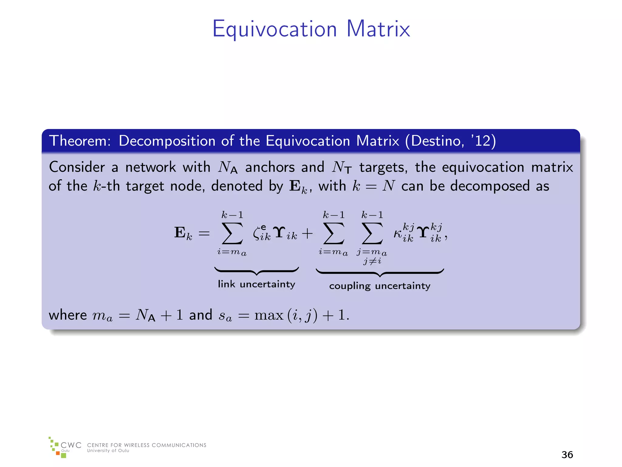
equivocation
anchor-to-target information
target-to-target
39](https://image.slidesharecdn.com/positioningseminar2012-121023023030-phpapp02/75/Positioning-seminar-2012-39-2048.jpg)
![Information of NLOS links
- Discard or do not discard? -
0.15
PEBLOS
PEBN LOS
PEBLOS with incompletion
0.125
Mean-square-error, MSE [m2 ]
0.1
Answer: Do not discard NLOS!
0.075
0.05
0.025
0 5 10 15 20 25 30 35 40 45 50
Probability of NLOS links, pN LOS [%]
Simulation: NA = 4 anchors, NT = 10 targets, σd = 0.3 meters, bMAX = 3 meters. Full connectivity.
ˆ
Metric: MSE = E{(Z − Z)2 }
41](https://image.slidesharecdn.com/positioningseminar2012-121023023030-phpapp02/75/Positioning-seminar-2012-41-2048.jpg)
![Non-Cooperative Positioning
Scenario of Non-cooperative Positioning
8
Anchor node
Target node
6
4
y-coordinate, [m]
2
0
−2
−4
−6
−8
−8 −6 −4 −2 0 2 4 6 8
x-coordinate, [m]
42](https://image.slidesharecdn.com/positioningseminar2012-121023023030-phpapp02/75/Positioning-seminar-2012-42-2048.jpg)

![Illustration of the Null-Space Analysis
- Distance contraction principle -
Exact ranging Positive ranging errors
8 8
Anchor node Anchor node
Target node Target node
6 Global optimum 6 Global optimum
4 4
y-coordinate, [m]
y-coordinate, [m]
2 2
0 0
−2 −2
−4 −4
−6 −6
−8 −8
−8 −6 −4 −2 0 2 4 6 8 −8 −6 −4 −2 0 2 4 6 8
x-coordinate, [m] x-coordinate, [m]
Negative ranging errors Error in the null-space of the angle-kernel
8 8
Anchor node Anchor node
Target node Target node
6 Global optimum 6 Global optimum
4 4
y-coordinate, [m]
y-coordinate, [m]
2 2
0 0
−2 −2
−4 −4
−6 −6
−8 −8
−8 −6 −4 −2 0 2 4 6 8 −8 −6 −4 −2 0 2 4 6 8
x-coordinate, [m] x-coordinate, [m]
47](https://image.slidesharecdn.com/positioningseminar2012-121023023030-phpapp02/75/Positioning-seminar-2012-47-2048.jpg)
![Robust Non-Cooperative Positioning
- Distance contraction based algorithms -
Algorithm 1 WC-DC Algorithm 2 NLS-DC
1: ˜
Measurements, {di }, 1: ˜
Measurements, {di },
2: Anchor positions, PA 2: Anchor positions, PA
3: Estimate a feasible region, BD 3: Estimate a feasible region, BD
4: z0 ← BD ;
ˆ 4: z0 ← BD ;
ˆ
5: ˆ
Ω ← O([PA ; z0 ]);
ˆ 5: ˆ
Ω ← O([PA ; z0 ]);
ˆ
6: ρ ← arg min
ˆ ˆˆˆ
ρ Ω ρT ; 6: ρ ← arg min
ˆ ˆˆˆ
ρ Ω ρT ;
ρ∈RNA
ˆ ρ∈RNA
ˆ
s.t. ˜
di + ρi ≤ 0 ∀i s.t. ˜
di + ρi ≤ 0 ∀i
ˆ ˜
7: [ω dc ]i ← ρi /di ; NA
˜ ˆ ˆ
7: z ← arg min
ˆ (di − ρi − di )2 .
8: z ← ω dc PA .
ˆ ηˆ
z∈R i=1
48](https://image.slidesharecdn.com/positioningseminar2012-121023023030-phpapp02/75/Positioning-seminar-2012-48-2048.jpg)
![Non-Cooperative Positioning
- Algorithm comparisons -
Comparison of Different Localization Algorithms
- non-cooperative network -
3.75
TS-WLS
3.5 WC-DC
NLS-DC
3.25 PEBNLOS
3
Location accuracy, ε [m]
2.75
2.5
¯
2.25
2
1.75
1.5
1.25
1
0.75
0.5
0.25
0 1 2 3 4 5
Maximum Bias, bMAX [m]
Network: Area (14.14 × 14.14) [m2 ], 4 anchors (square location), 10 targets (inside the anchors).
Noise: σd = 0.3 [m], pNLOS = 1. Location accuracy: ε =
¯ ˆ
E{(Z − Z)2 } [m] .
49](https://image.slidesharecdn.com/positioningseminar2012-121023023030-phpapp02/75/Positioning-seminar-2012-49-2048.jpg)
![Non-Cooperative Positioning
- Algorithm comparisons -
Comparison of Different Localization Algorithms
- non-cooperative network -
2
TS-WLS
WC-DC
NLS-DC
1.75 PEBN LOS
Location accuracy, ε [m]
1.5
¯
1.25
1
0.75
0.5
0.25
0 0.25 0.5 0.75 1
Probability of NLOS, pNLOS
Network: Area (14.14 × 14.14) [m2 ], 4 anchors (square location), 10 targets (inside the anchors).
Noise: σd = 0.3 [m], bmax = 3 [m]. Location accuracy: ε =
¯ ˆ
E{(Z − Z)2 } [m].
50](https://image.slidesharecdn.com/positioningseminar2012-121023023030-phpapp02/75/Positioning-seminar-2012-50-2048.jpg)
![Cooperative Algorithm
Scenario of Cooperative Positioning
8
Anchor node
Target node
6
4
y-coordinate, [m]
2
0
−2
−4
−6
−8
−8 −6 −4 −2 0 2 4 6 8
x-coordinate, [m]
51](https://image.slidesharecdn.com/positioningseminar2012-121023023030-phpapp02/75/Positioning-seminar-2012-51-2048.jpg)
![Cooperative Positioning
- R-GDC optimization performance -
R-GDC Performance in Large Scale Networks
- cooperative network -
0.65
R-GDC
0.6 PEBLOS
0.55
0.5
Location accuracy, ε [m]
0.45
¯
0.4
0.35 NT = 50
0.3
0.25 NT = 100
0.2 NT = 200
0.15
0.1
0.05
0.2 0.3 0.4 0.5 0.6 0.7 0.8 0.9 1
Meshness ratio, m
Network: Area (14.14 × 14.14) [m2 ], 4 anchors (square location), NT targets (inside the anchors).
Noise: σd = 0.3 [m]. s Location accuracy: ε =
¯ ˆ
E{(Z − Z)2 } [m].
56](https://image.slidesharecdn.com/positioningseminar2012-121023023030-phpapp02/75/Positioning-seminar-2012-56-2048.jpg)
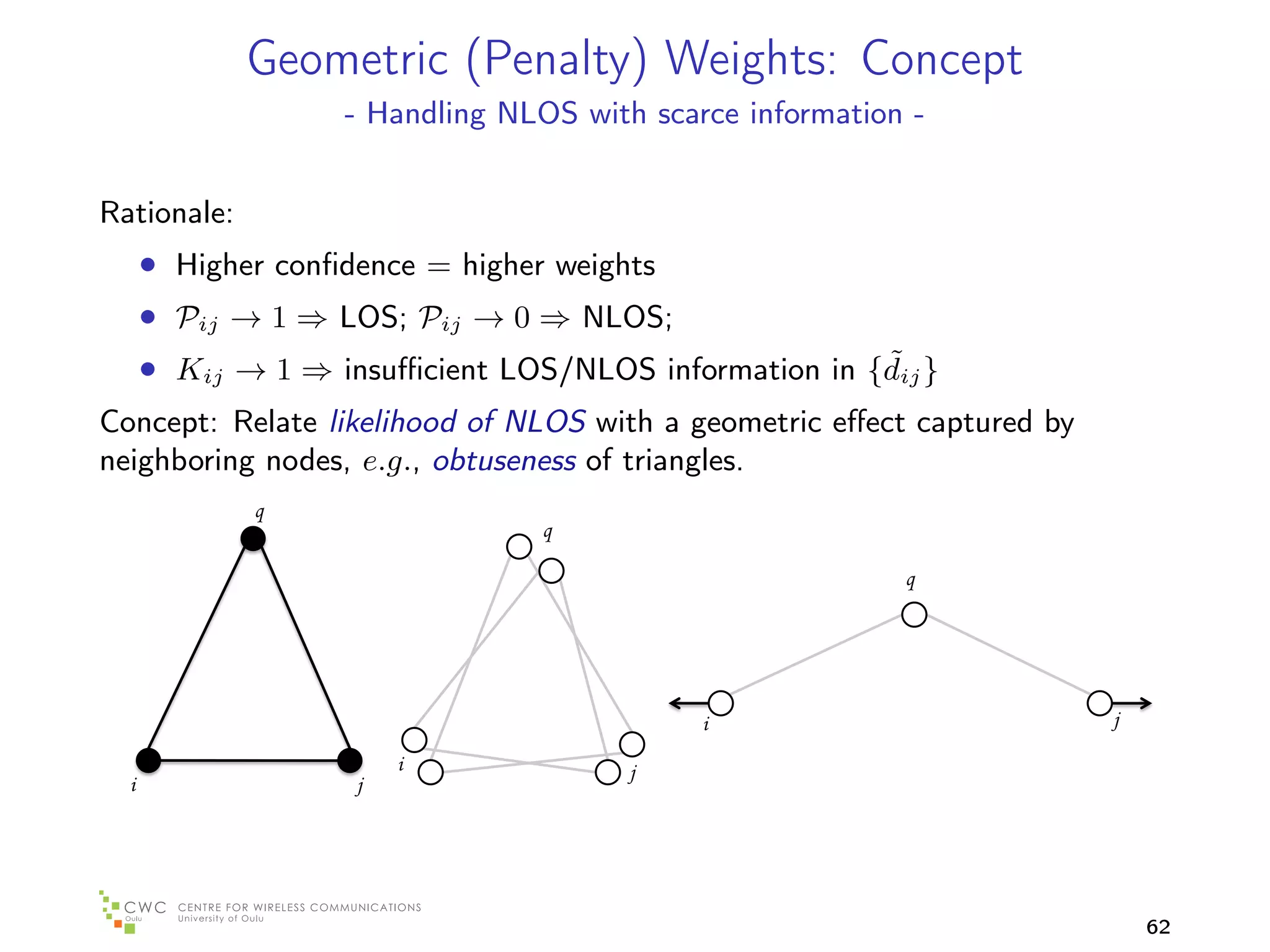
![Stochastic (Dispersion) Weighing Function
- The intuition behind: sort categorical data -
Pool of objects Scale
Which unit:? [γ]
Object characteristics
• shape, σ
• density, K
Metric
• weight: w = f (σ, K; γ)
60](https://image.slidesharecdn.com/positioningseminar2012-121023023030-phpapp02/75/Positioning-seminar-2012-60-2048.jpg)
![Maximum Entropy Criteria
Our context:
• Categories → (K, σ )
ˆ
• Sample → zij = (Kij , σij )
ˆ
• Weight of zij → wij
• Population → Z = [Kmin , Kmax ] × [ˆmin , σmax ]
σ ˆ
Diversity of the the objects by the weights is
Kmax ˆ
σmax
H(γ) = w(S, r; γ) · ln (w(S, r; γ)) dS
r=Kmin σ
ˆ min
• Uncertainty analysis: measure wij and compute H (diversity)
• Weight optimization: compute wij that maximizes H (diversity)
γopt = arg max H(γ)
γ∈R+
61](https://image.slidesharecdn.com/positioningseminar2012-121023023030-phpapp02/75/Positioning-seminar-2012-61-2048.jpg)

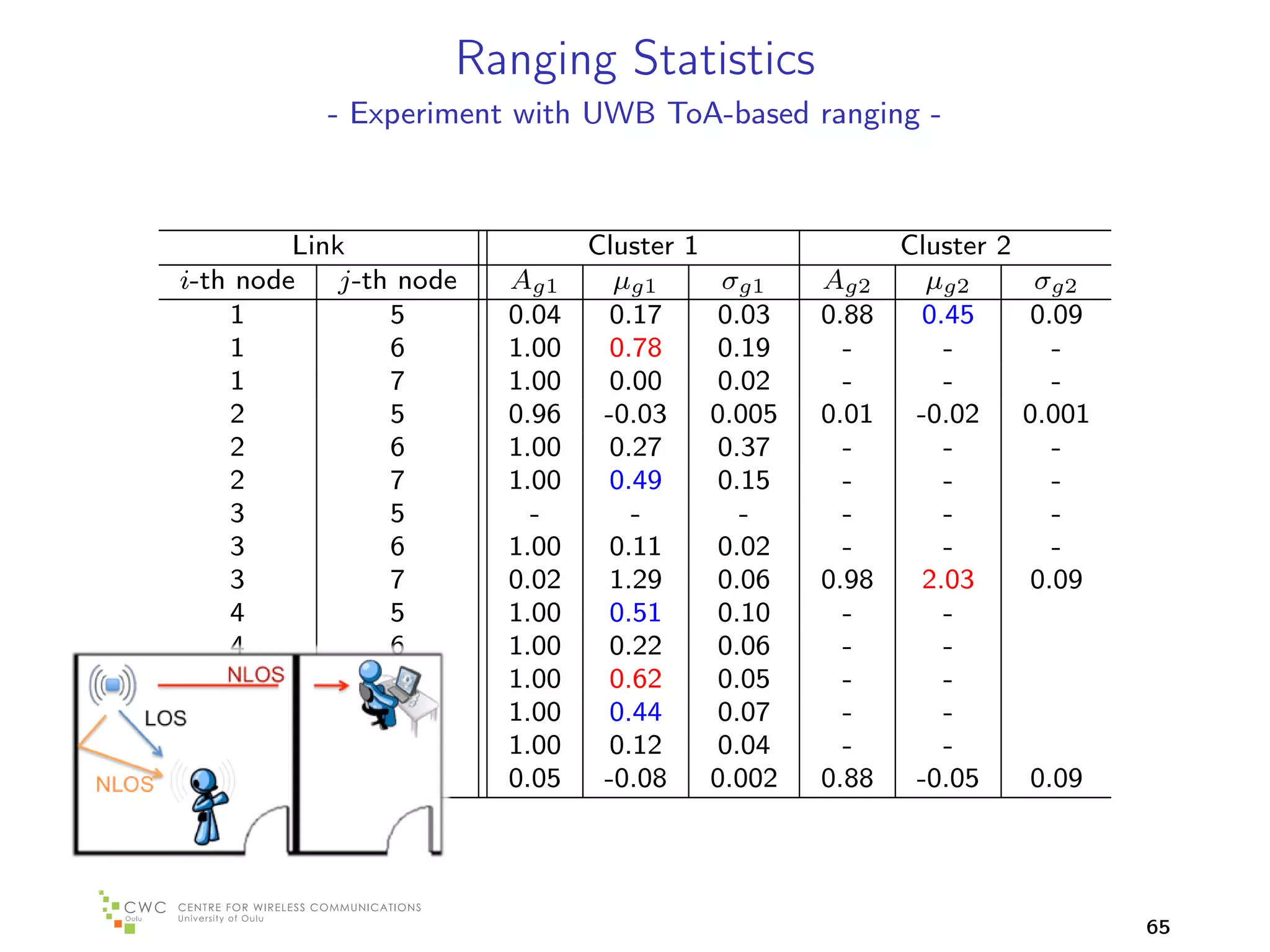
![Distance Estimation Indoors
- Experiment with UWB ToA-based ranging -
Localization Test
- network -
12
Anchor
11 Target
p4 p2
10 eLAB p5
9
8 p6
y-coordinate [m]
7
p7
6
5
4 p3
p1
3
2
1
0
0 1 2 3 4 5 6 7 8 9 10 11 12
x-coordinate, [m]
CWC/Oulu Installations
64](https://image.slidesharecdn.com/positioningseminar2012-121023023030-phpapp02/75/Positioning-seminar-2012-64-2048.jpg)
![Non-Cooperative Positioning
- Experiment with UWB ToA-based ranging -
Localization Test
- non-cooperative -
12
11
p4 p2
10 p5
9
8 p6
y-coordinate [m]
7
p7
6
5
4 p3
p1
3
2
Anchor
Target
C-NLS modified
1 DC-NLS
DC-WC
0
0 1 2 3 4 5 6 7 8 9 10 11 12
x-coordinate, [m]
Metric NLS-DC WC-DC C-NLS modified
Average RMSE [m] 0.29 0.27 0.38
Average CEP-50 [m] 0.24 0.23 0.31
Average CEP-95 [m] 0.41 0.37 0.47
66](https://image.slidesharecdn.com/positioningseminar2012-121023023030-phpapp02/75/Positioning-seminar-2012-66-2048.jpg)
![Cooperative Positioning
- Experiment with UWB ToA-based ranging -
Localization Test
- cooperative -
12
p9
11
p4 p2
10 p7
9
8 p8
y-coordinate [m] p5
7
p10
6
5
4 p3
p1
3
p12
p11
2
Anchor
Target p6
SDP - C
1 SDP - LOESS
R-GDC - DP
0
0 1 2 3 4 5 6 7 8 9 10 11 12
x-coordinate, [m]
Metric R-GDC - DP SDP - LOESS SDP - C
Average RMSE [m] 0.29 0.33 0.40
Average CEP-50 [m] 0.16 0.27 0.37
Average CEP-95 [m] 0.46 0.56 0.63
67](https://image.slidesharecdn.com/positioningseminar2012-121023023030-phpapp02/75/Positioning-seminar-2012-67-2048.jpg)

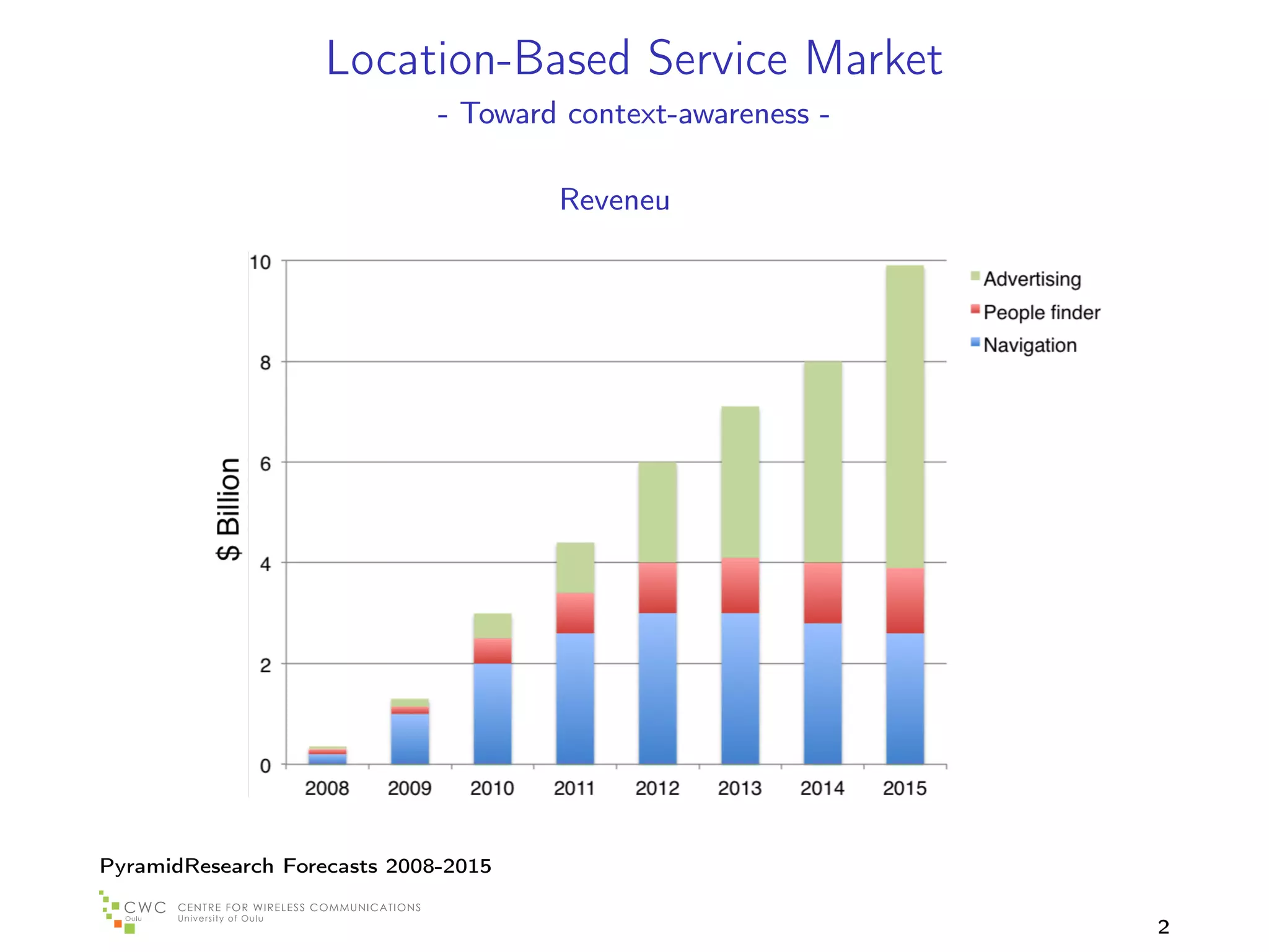
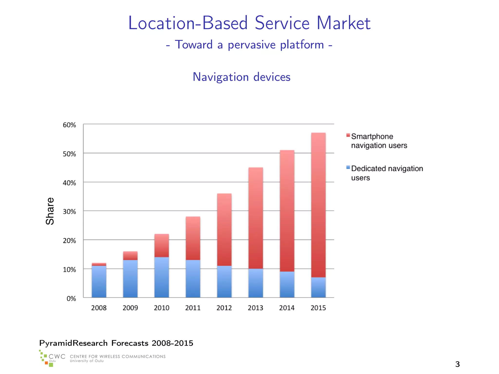
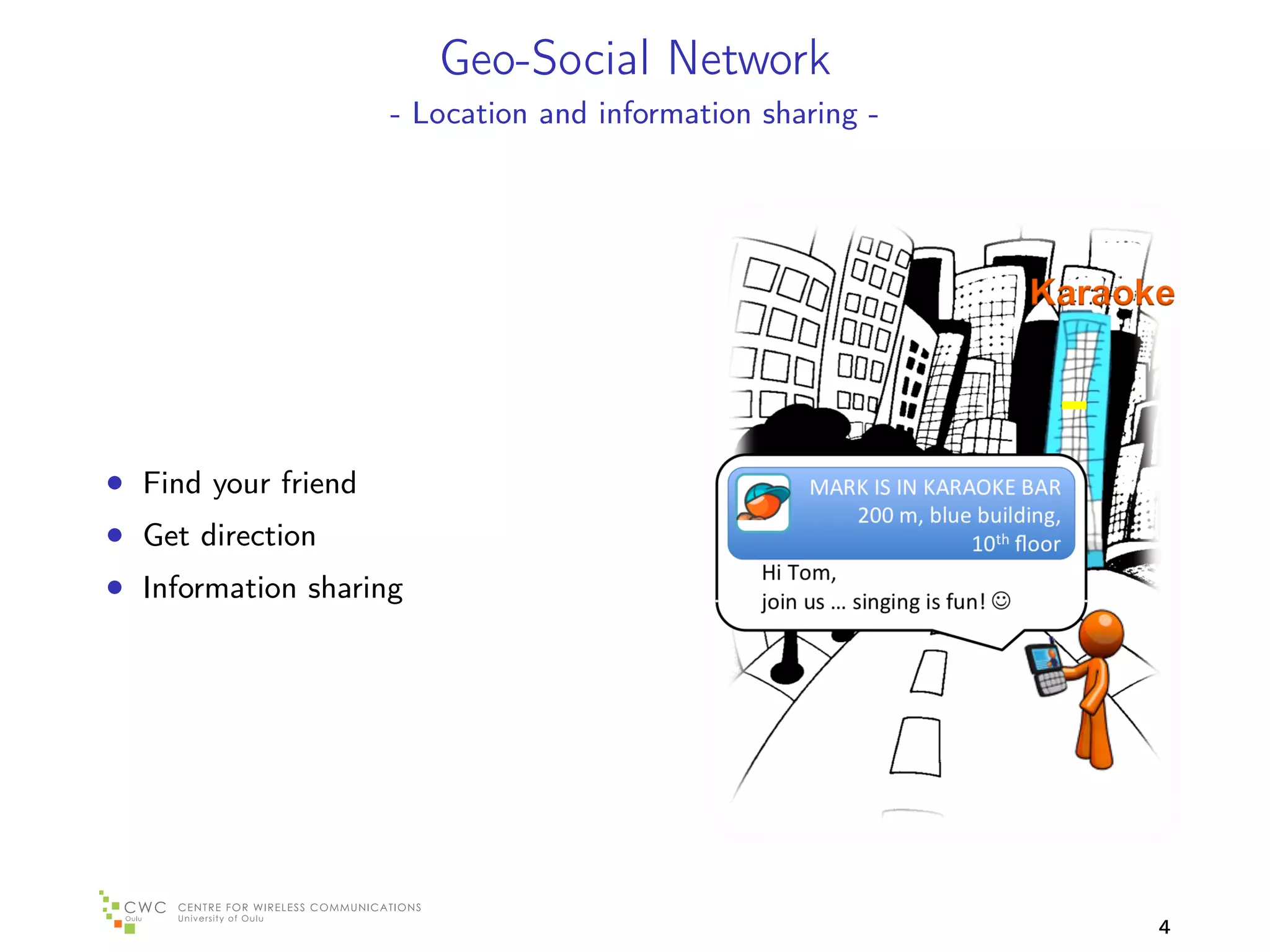
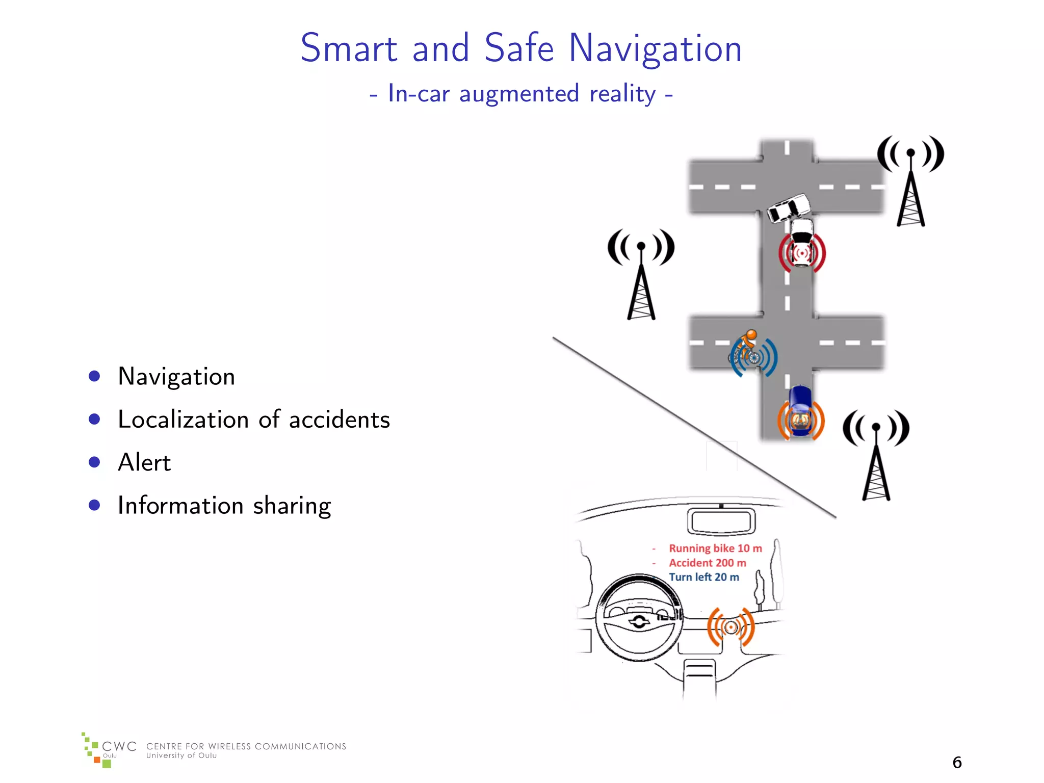
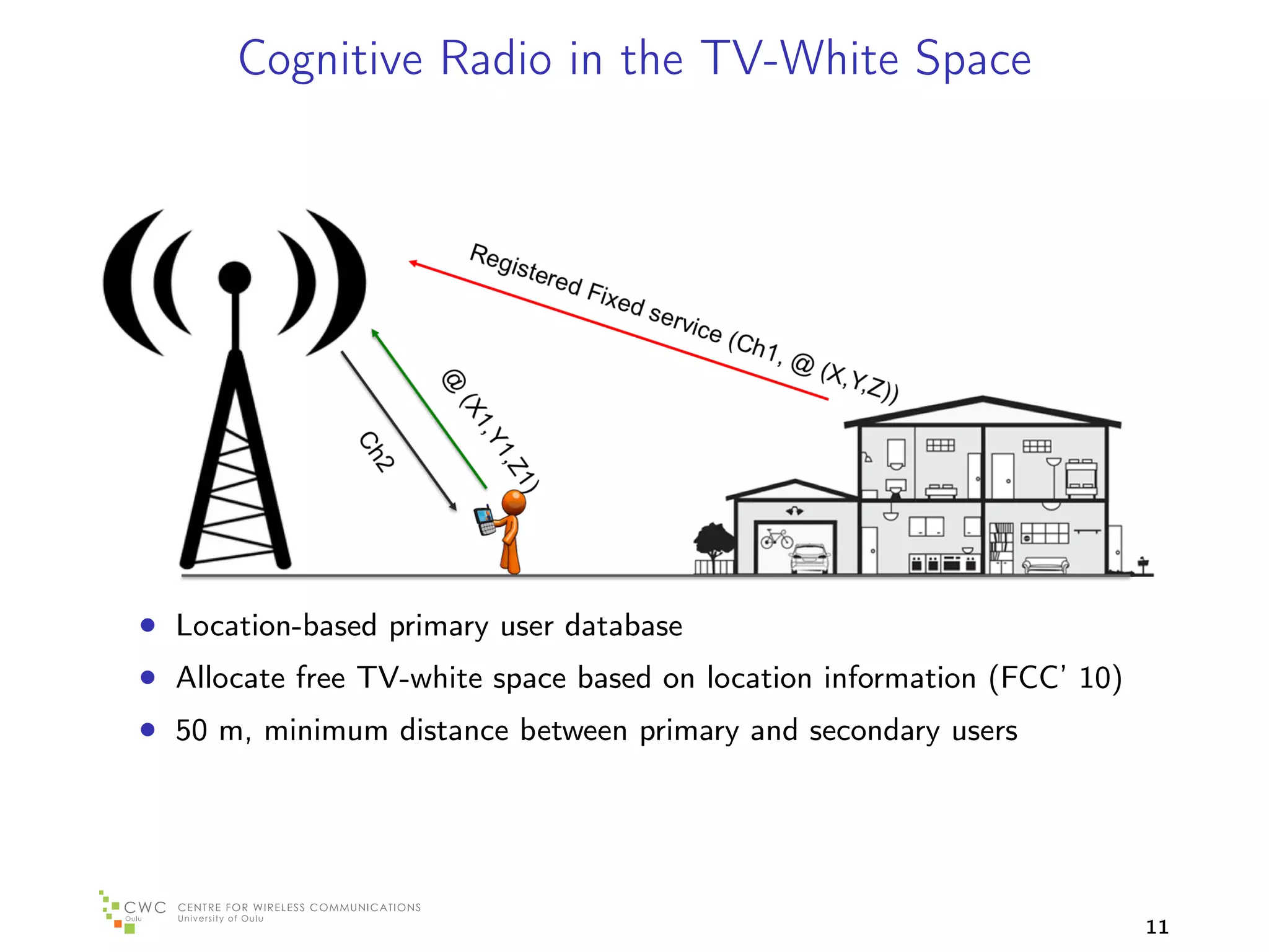
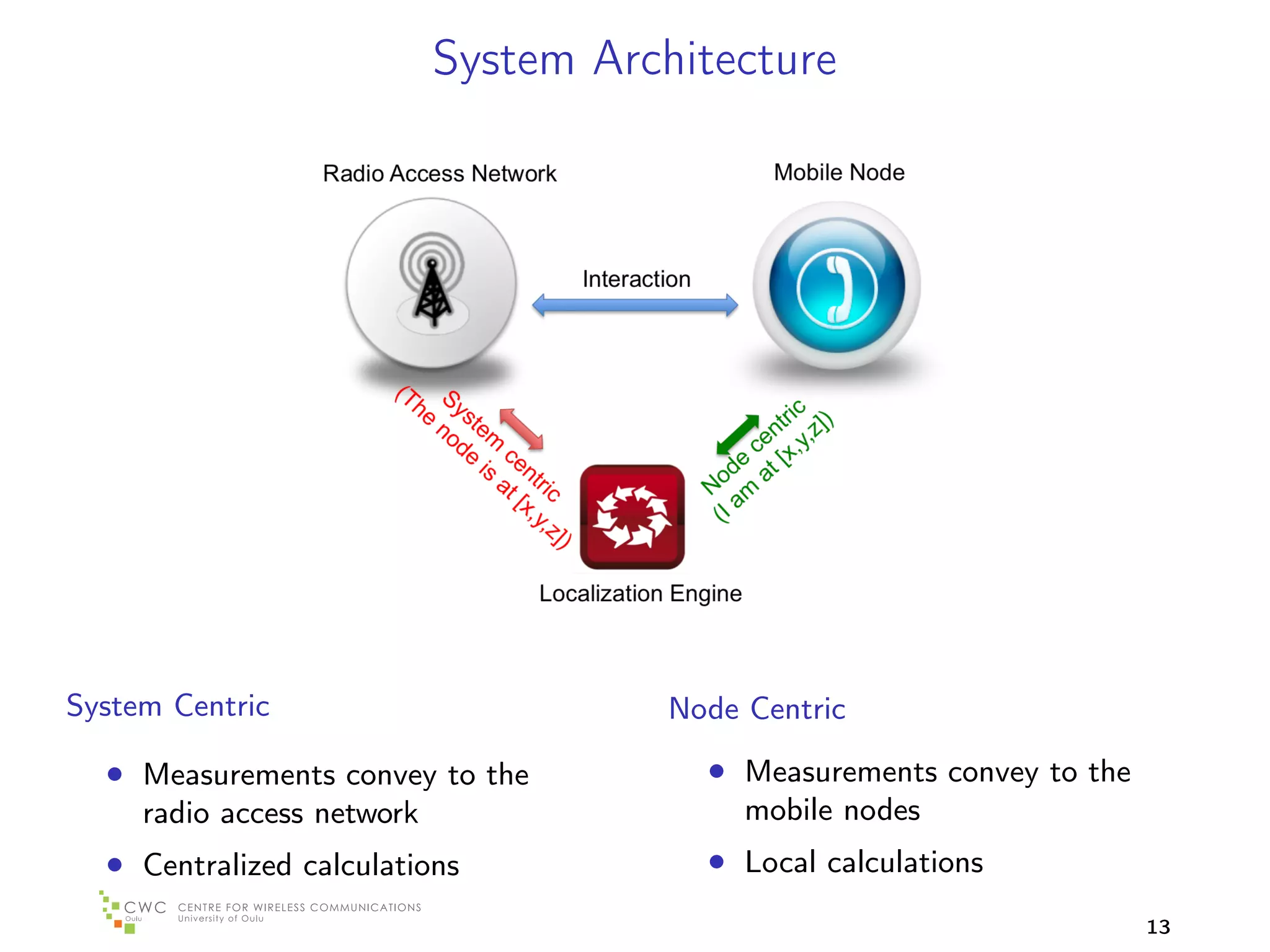
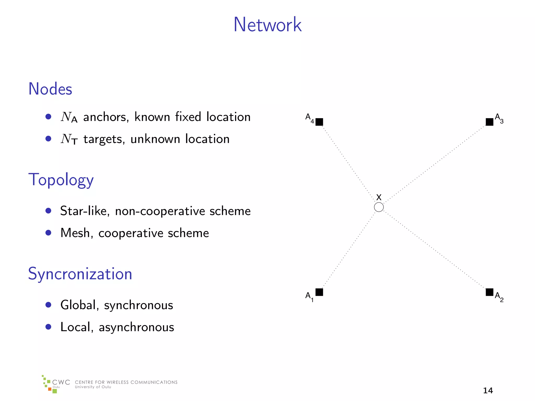
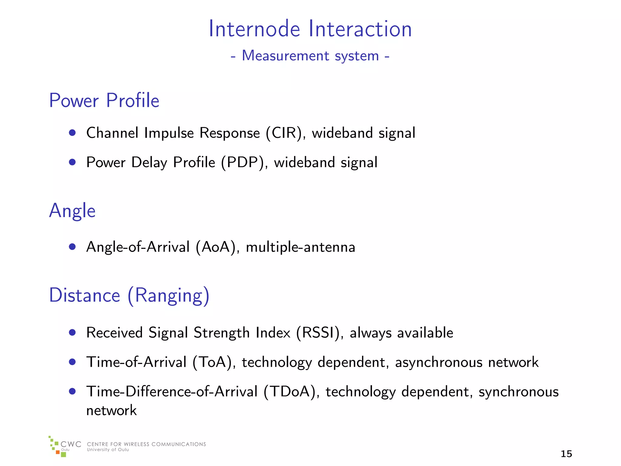
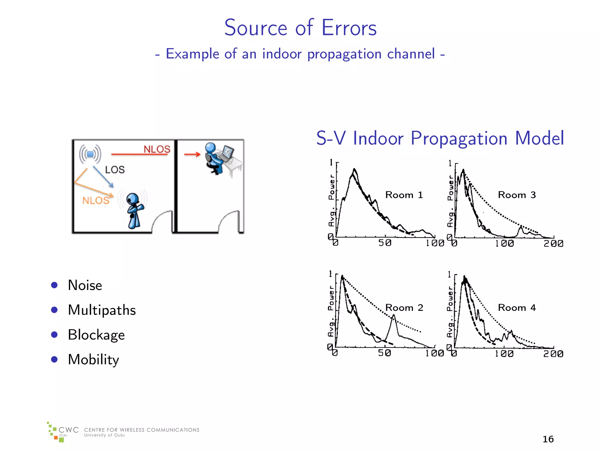
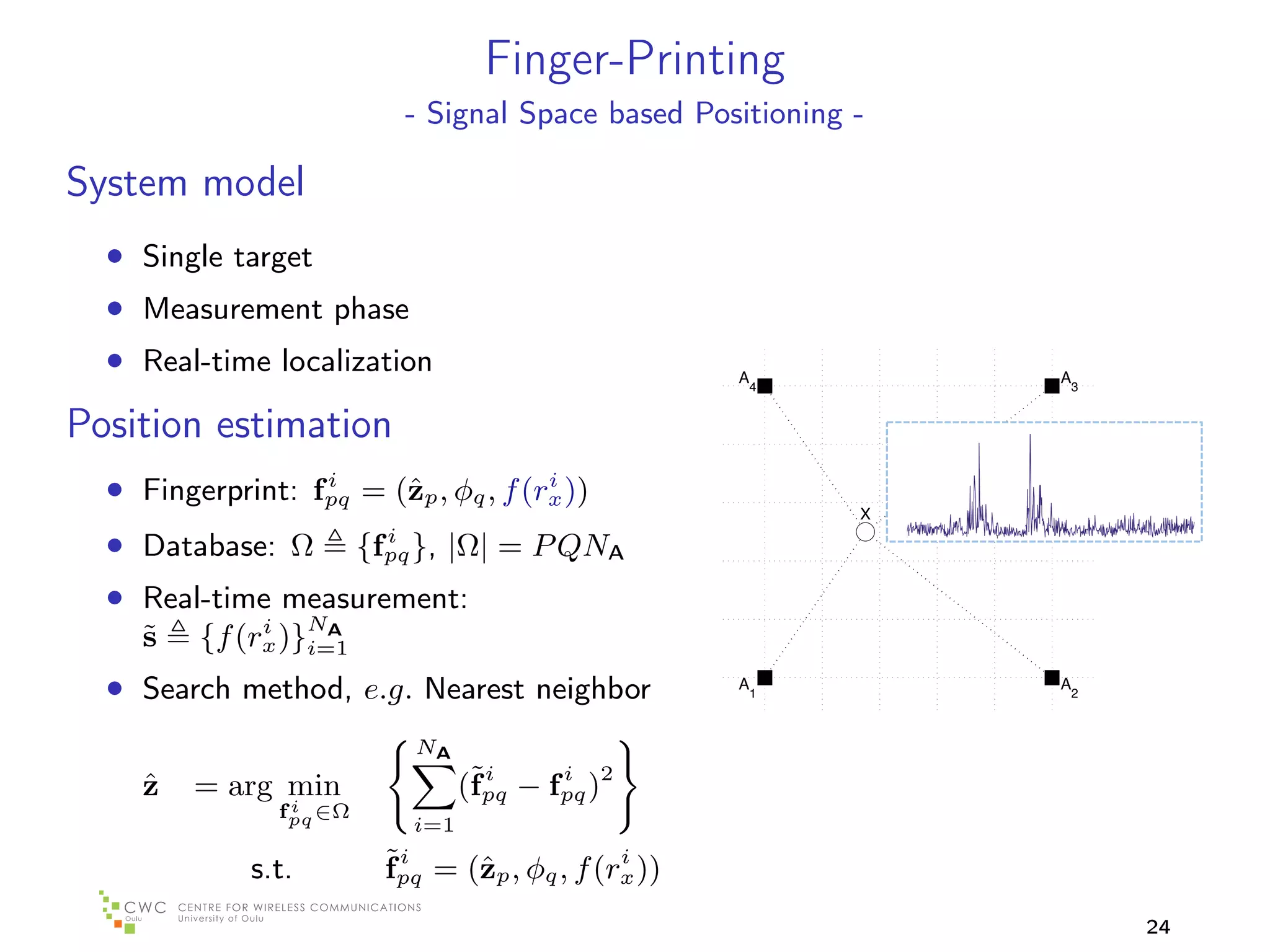
The document discusses location-based services and applications that utilize positioning systems. It describes several types of location-based services that are emerging, such as navigation assistance, geo-social networking, personalized advertising, and industrial monitoring. It also outlines key components of positioning systems, including network architecture, node interaction methods for measuring location like power profiling and angle of arrival, and sources of errors in indoor positioning.


![[CONTEXTS'11] A bayesian strategy to enhance the performance of indoor locali...](https://cdn.slidesharecdn.com/ss_thumbnails/contexts11abayesianstrategytoenhancetheperformanceofindoorlocalizationsystems-120611064501-phpapp01-thumbnail.jpg?width=640&height=640&fit=bounds)


![Coded Agents – with UiPath SDK + LangGraph [Virtual Hands-on Workshop]](https://cdn.slidesharecdn.com/ss_thumbnails/codedagentsdeck-251215155422-5497c599-thumbnail.jpg?width=640&height=640&fit=bounds)


