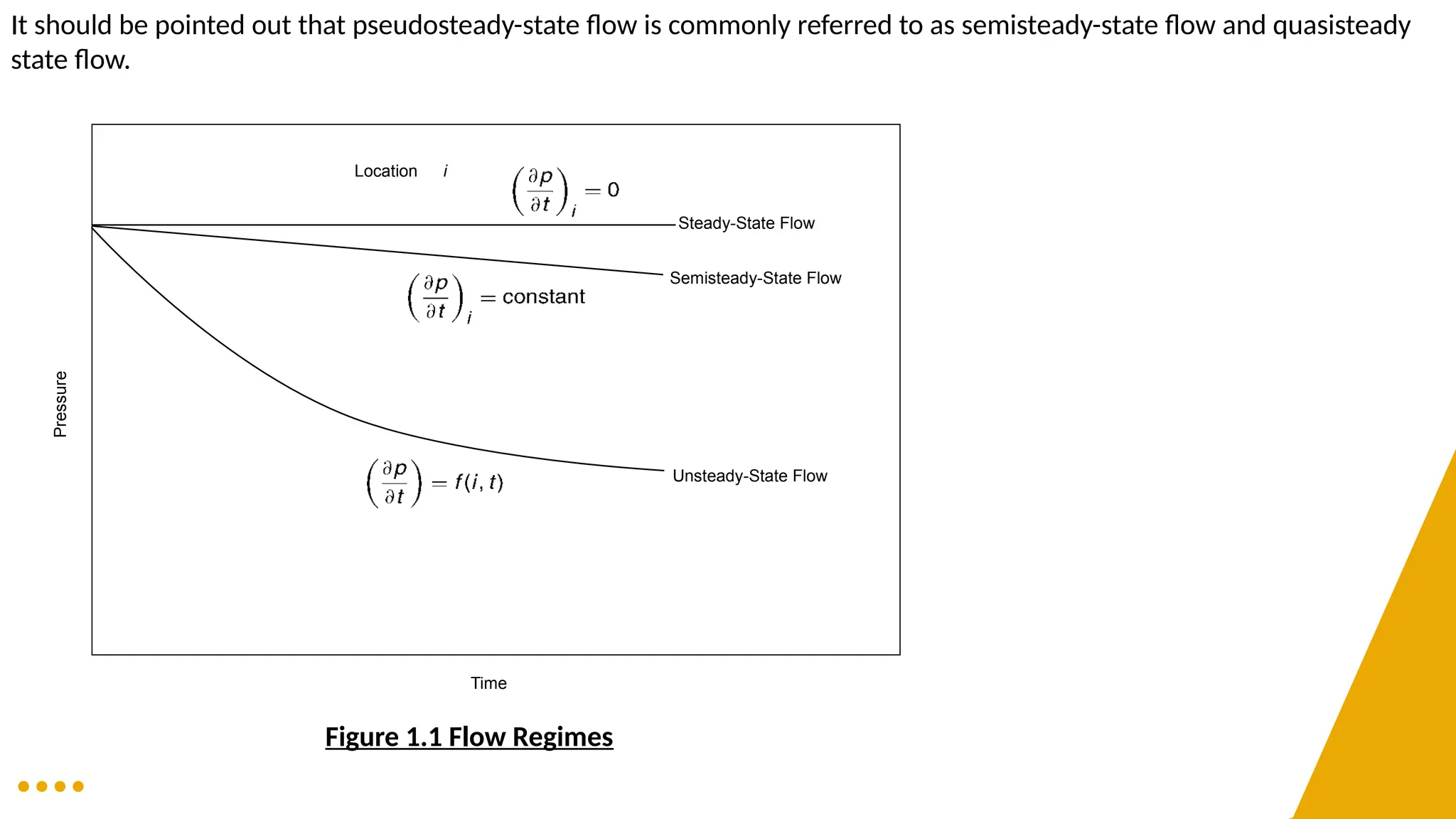
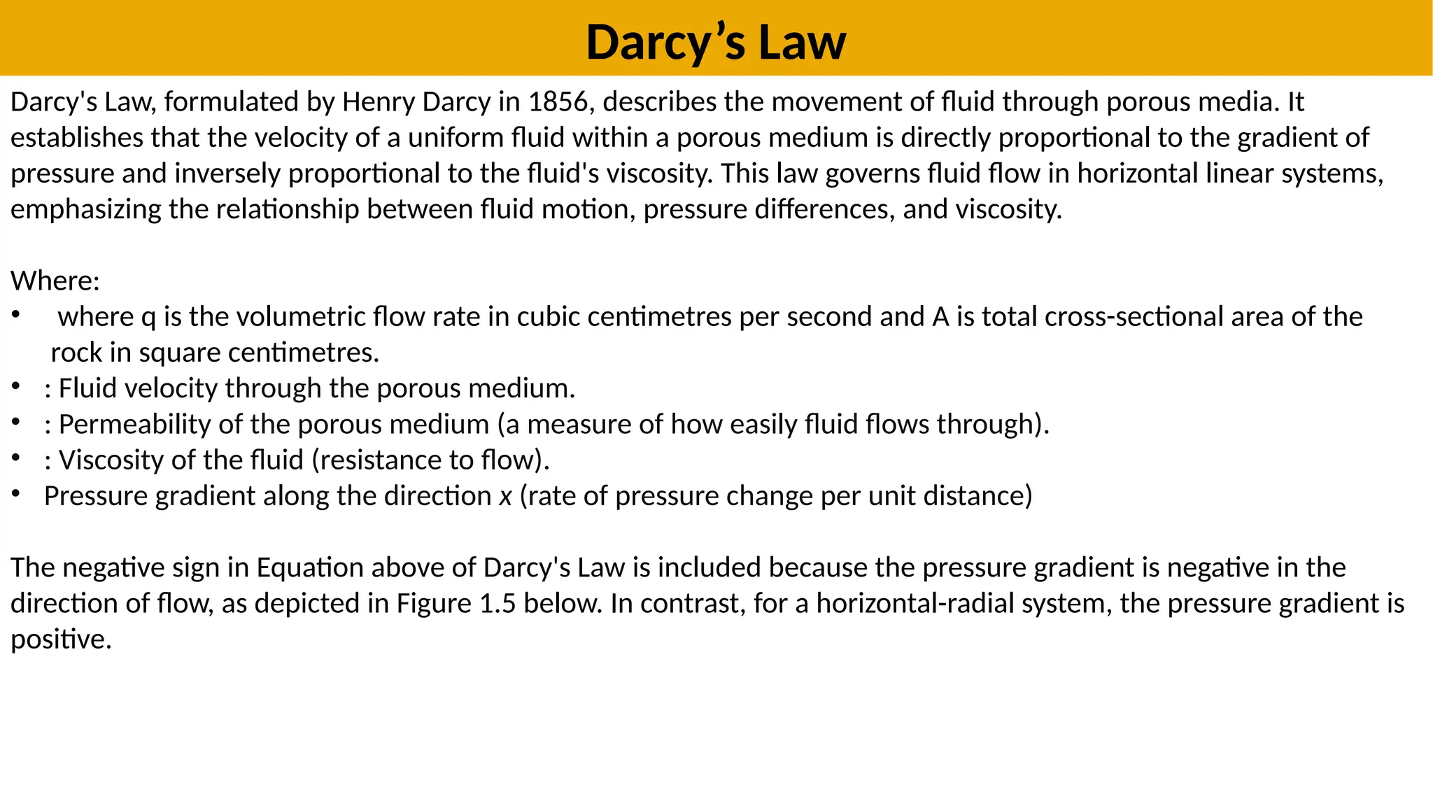
Introduction To
Flow In Porous
Media
The Introduction to Flow in Porous Media is divided
into 5 parts:
1. Fluid Flow in Porous Media.
2. Fluid Flow Equations.
3. Fluid and Rock Properties.
4. Reservoir Fluid Viscosities
5. Darcy’s Law.
Supervising Lecturer:
Dr Adegboyega B EHINMOWO
Course Outline
1. Fluid Flow In Porous Media
• Types Of Fluid in the Reservoir.
• Flow Regimes.
• Reservoir Geometry.
• Number of flowing fluids in the
Reservoir.
3. Fluid and Rock
Properties
• Properties of Natural Gas
• Rock Properties
• Formation Volume Factors
5. Darcy’s Law
• Types Of Fluid in the Reservoir.
• Flow Regimes.
• Reservoir Geometry.
• Number of flowing fluids in the
Reservoir.
2. Fluid Flow Equations
• Conservation of Mass equation.
• Momentum/Transport equation-
Darcy’s equation.
• Equation of State.
• Energy Equation.
4. Reservoir Fluid
Viscosities
• Water Viscosity
• Oil Viscosity
• Gas Viscosity
Fluid Flow In Porous Media
Flow in porous media is a very complex phenomenon and cannot be described as explicitly as flow
through pipes or conduits. It is rather easy to measure the length and diameter of a pipe and
compute its flow capacity as a function of pressure; however, in porous media flow is different in
that there are no clear-cut flow paths which lend themselves to measurement.
The analysis of fluid flow in porous media has evolved throughout the years along two fronts: the
experimental and the analytical.
Focusing on the analytical (mathematical) forms that are designed to describe the flow behaviour of
the reservoir fluids. The mathematical forms of these relationships will vary depending upon the
characteristics of the reservoir. These primary reservoir characteristics that must be considered
include:
● Types of fluids in the reservoir
● Flow regimes
● Reservoir geometry
● Number of flowing fluids in the reservoir.
Types Of Fluids
The isothermal compressibility coefficient is essentially the controlling factor in identifying the type of the
reservoir fluid. In general, reservoir fluids are classified into three groups:
1. Incompressible fluids;
2. Slightly compressible fluids
3. Compressible fluids.
The isothermal compressibility coefficient c is described mathematically by the following two
equivalent expressions:
In terms of fluid volume:
In terms of fluid density:
Where V and ρ are the volume and the density of the fluid, respectively.
Incompressible Fluids
An incompressible fluid is defined as the fluid whose volume (or density) does not change with
pressure, i.e.:
,
Incompressible fluids do not exist; this behaviour, however, may be assumed in some cases to
simplify the derivation and the final form of many flow equations.
Slightly Compressible Fluids
These “slightly” compressible fluids exhibit small changes in volume, or density, with changes in pressure.
Knowing the volume Vref of a slightly compressible liquid at a reference (initial) pressure pref, the changes in the
volumetric behaviour of this fluid as a function of pressure p can be mathematically described by integrating the
‘fluid volume compressibility equation’ to give:
where
P = pressure, psia
V = volume at pressure p,
Pref = initial (reference) pressure, psia
Vref = fluid volume at initial (reference) pressure, psia
Compressible Fluids
These are fluids that experience large changes in volume as a function of pressure. All gases are considered compressible
fluids, the isothermal compressibility of any compressible fluid is described by the following expression:
Flow Regimes
There are basically three types of flow regimes that must be recognized in order to describe the fluid flow behaviour
and reservoir pressure distribution as a function of time. These three flow regimes are:
1. Steady-state flow.
2. Unsteady-state flow.
3. Pseudosteady-state flow.
Steady-state flow
The flow regime is identified as a steady-state flow if the pressure at every location in the reservoir remains constant,
i.e. does not change with time.
Mathematically, this condition is expressed as:
This equation states that the rate of change of pressure p with respect to time t at any location i is zero. In
reservoirs, the steady-state flow condition can only occur when the reservoir is completely recharged and
supported by strong aquifer or pressure maintenance operations.
Unsteady-state flow
Unsteady-state flow (frequently called transient flow) is defined as the fluid flowing condition at which the rate
of change of pressure with respect to time at any position in the reservoir is not zero or constant. This definition
suggests that the pressure derivative with respect to time is essentially a function of both position i and time t,
thus:
Pseudosteady-state flow
When the pressure at different locations in the reservoir is declining linearly as a function of time, i.e., at a
constant declining rate, the flowing condition is characterized as pseudosteady-state flow. Mathematically, this
definition states that the rate of change of pressure with respect to time at every position is constant, or:
It should be pointed out that pseudosteady-state flow is commonly referred to as semisteady-state flow and quasisteady
state flow.
Time
Unsteady-State Flow
Location i
Semisteady-State Flow
Steady-State Flow
Pressure
Figure 1.1 Flow Regimes
Reservoir Geometry
The shape of a reservoir has a significant effect on its flow behaviour. Most reservoirs have irregular boundaries and a
rigorous mathematical description of their geometry is often possible only with the use of numerical simulators.
However, for many engineering purposes, the actual flow geometry may be represented by one of the following flow
geometries:
• Radial Flow;
• Linear Flow;
• Spherical and Hemispherical Flow.
Radial Flow
In the absence of severe reservoir heterogeneities, flow into or away from a wellbore will follow radial flow lines a
substantial distance from the wellbore. Because fluids move toward the well from all directions and coverage at the
wellbore, the term radial flow is used to characterize the flow of fluid into the wellbore.
Linear Flow
Linear flow occurs when flow paths are parallel and the fluid flows in a single direction. In addition, the cross-sectional area to
flow must be constant.
Spherical and hemispherical flow
Depending upon the type of wellbore completion configuration, it is possible to have spherical or hemispherical flow near
the wellbore. A well with a limited perforated interval could result in spherical flow in the vicinity of the perforations as
illustrated in Figure 1.2 . A well which only partially penetrates the pay zone, as shown in Figure 1.3 could result
in hemispherical flow. The condition could arise where coning of bottom water is important.
LINEAR RADIAL SPHERICAL
Figure 1.2 Common Flow Geometries
Wellbore
p
wf
Side View Flow Lines
Figure 1.3 Spherical flow due to limited entry
Number Of Flowing Fluids In the Reservoir
The mathematical expressions that are used to predict the volumetric performance and pressure behaviour of
a reservoir vary in form and complexity depending upon the number of mobile fluids in the reservoir. There
are generally three cases of flowing system:
1. Single-phase flow (oil, water, or gas);
2. Two-phase flow (oil–water, oil–gas, or gas–water);
3. Three-phase flow (oil, water, and gas).
The description of fluid flow and subsequent analysis of pressure data becomes more difficult as the number
of mobile fluids increases.
Fluid Flow Equations
The fluid flow equations that are used to describe the flow behaviour in a reservoir can take many forms depending
upon the combination of variables presented previously (i.e., types of flow, types of fluids, etc.). By combining the
conservation of mass equation with the transport equation (Darcy’s equation) and various equations of state, the
necessary flow equations can be developed.
Based on these classifications, the equation of fluid flow is related to following laws. They are:
1. Conservation of Mass Equation.
2. Momentum/Transport Equation
3. Equation of State.
4. Energy Equation.
Conservation Of Mass Equation
The conservation of mass states that “mass can neither be created nor destroyed”. That is, the net mass crossing a system
must be balanced by either an accumulation or depletion of the mass in the system.
Derivation of the Conservation of Mass Equation
From the Lagrangian from where mass variation is zero
Conservation Of Momentum Equation
This is a general equation that governs the motion of fluids (and other fluids) at the microscopic level. It's a
complex equation derived from the Navier-Stokes equations, which account for factors like inertia, viscosity,
pressure gradients, and external forces.
• The momentum equation, an expression of Newton’s second law of motion, represents the transient force
balance on the fluid within a slice of the pipeline cross-section.
• The left side, is mass times acceleration per unit volume of fluid (there is a velocity change in time, as well
as a change as it moves in distance).
• The right side (RHS) represents the forces acting on a unit mass of fluid.
• The first RHS term, is the net force imposed by the pressure gradient.
• The second RHS term, is the force of gravity on the element as it moves in the vertical direction (due to the
slope of the pipeline) .
• The final term is the frictional force that acts in a direction opposite to the velocity.
• Equation of states are variables that depend upon the state of a system, each of state is
Equation Of State
………………………. (1)
• For gases at reasonably high temperatures or low pressures the equation of state is written as;
……………………. (2)
Where R is gas constant
• For Perfect (ideal) gases, ……………………….(3)
• Then for Incompressible fluids …................(4)
Energy Equation
The energy equation is a restatement of thermodynamics which states that, “the total energy change in a system
equals the difference between heat transferred to the system and work done by the system on it’s surroundings.
The Lagrangian form of this law is given by:
Where = heat transfer
and = work done
Total Energy
We can write the total energy as;
Fluid and Rock Properties
Reservoir fluids are the fluids that exist in a petroleum reservoir. The fluid type must be determined very
early in the life of a reservoir (often before sampling or initial production) because fluid type is the critical
factor in many of the decisions that must be made about producing the fluid from the reservoir.
Reservoir-fluid properties play a key role in the design and optimization of injection/production strategies
and surface facilities for efficient reservoir management. Inaccurate fluid characterization often leads to
high uncertainties in in-place-volume estimates and recovery predictions, and hence affects asset value.
Indeed, evaluating reservoir fluids is an important aspect of prospect evaluation, development planning,
and reservoir management.
Although many different types of fluid exist, the composition of the reservoir fluids provides important
information that can influence the recovery process. Prior to production, these measurements will
represent static data but once production commences, dynamic data will become available and variations
in fluid composition, which are effective on a production timescale, will become apparent. Reservoir
fluids, including heavy oil, vary greatly in composition.
In some fields, the fluid is in the gaseous state and in others it is in the liquid state but gas and liquid frequently coexist in a
reservoir. The rocks which contain these reservoir fluids also vary considerably in composition and in physical and flow
properties and this can serve to complicate the sampling procedure. Other factors, such as producing area, height of the
column of hydrocarbon fluid, fracturing or faulting, and water production also serve to distinguish one reservoir from
another. The combination of all these factors affects the choice of sampling methods and preparations for sampling.
Properties of Natural Gas
Natural gas is a combustible gas produced from the subsurface formation. The physical properties of natural gas such as
composition, specific gravity, compressibility factor, viscosity, etc. are fundamental data in petroleum reservoir
calculations. Natural gas is a mixture of lighter paraffin hydrocarbon and nonhydrocarbon gases. The composition of
natural gas is the main influencing factor of its physical properties and commercial value.
Knowledge of pressure-volume-temperature (PVT) relationships and other physical and chemical properties of gases is
essential for solving problems in natural gas reservoir engineering. These properties include:
• Apparent molecular weight, Ma • Specific gravity, γg • Compressibility factor, z
• Density, ρg • Specific volume, v • Isothermal gas compressibility coefficient, cg
• Gas formation volume factor, Bg • Gas expansion factor, Eg • Viscosity,
The above gas properties may be obtained from direct laboratory measurements or by prediction from generalized
mathematical expressions.
• Equation of State
• Behavior of Ideal Gas
There are no ideal gases in nature. The term ‘ideal gas’ is a hypothetical gas. An ideal gas has the following
properties:
1. The volume occupied by the molecules is insignificant with respect to the volume occupied by the gas.
2. There are no attractive or repulsive forces between the molecules or between the molecules and the walls of the
container.
3. All collisions of molecules are perfectly elastic, i.e. there is no loss of internal energy upon collision.
Combining the equations of Boyle, Charles and Avogadro will give an equation of state for an ideal gas:
In the equation above, V is the volume of n moles of gas at temperature T and pressure p, R is a constant and is
called the universal gas constant. It is the same for all ideal gases.
Behavior of Real Gas
The behavior of most real gases does not deviate drastically from the behavior predicted by the ideal gas
equation. So. the best way of writing an equation of state for a real gas is to insert a correction factor into the
ideal gas equation.
Where the correction factor, z, is known as the compressibility factor and the equation is known as the
compressibility equation of state or simply real gas equation of state. Compressibility factor is also known as gas
deviation factor or z-factor. It is the ratio of the volume occupied by a gas at given pressure and temperature to
the volume occupied by the gas at the same pressure and temperature if it behaves like an ideal gas. The z-factor
is not a constant but varies with changes in gas composition, temperature and pressure. It must be determined
experimentally. At low pressures, the molecules of gas are relatively far apart and the conditions of ideal gas
behavior are more likely to be met. The compressibility factor approaches 1.0 at low pressures. At moderate
pressures, the molecules are close enough to exert some attractions between them, the z factor is less than 1.0.
However, at higher pressures, the molecules are forced close together and repulsive forces come into play and
the z-factor is greater than 1.0.
Gas Formation Volume Factor
The gas formation volume factor is the volume occupied in the reservoir by a unit volume of gas at standard
conditions (, 0.101325 MPa). The- formation volume factor of a gas may be calculated as the volume occupied by
the gas at reservoir temperature and pressure divided by the volume occupied by the same mass of gas at standard
conditions
Where, Bg is the formation volume factor, / (standard), Vg is the volume occupied by n moles of gas at reservoir
conditions, , Vsc is the volume occupied by n moles of gas at standard conditions, (standard). The volume of n moles
of a gas at reservoir conditions may be obtained from the compressibility equation of state.
T is the reservoir temperature, K and p is the reservoir pressure in MPa. The volume of the same number of moles
of the gas at standard conditions, Tsc and Psc can be obtained using the ideal gas law.
Thus, the formation volume factor for the gas is:
Since psc = 0.101325 MPa, Tsc = 273 + 20 = 293 K, then
T is the reservoir temperature,.
• Porosity
• Permeability
• Capillary
• Saturation
• Wettability
• Compressibility
POROSITY
For rock to contain petroleum and later allow petroleum to flow, it must have certain physical characteristics.
Obviously, there must be some spaces in the rock in which the petroleum can be stored. If rock has openings, voids
and spaces in which liquid and gas may be stored, it is said to be porous .For a given volume of rock, the ratio of the
open space to the total volume of the rock is called porosity, The porosity may be expressed a decimal fraction but is
most often expressed as a percentage eg, if 100 cubic feet of rock contains many tiny pores and spaces which
together have a volume of 10 the porosity of the rock is 10%.
As the sediments were deposited and the rocks were being formed during past geological times, some void spaces
that developed became isolated from the other void spaces by excessive cementation. Thus, many of the void
spaces are interconnected while some of the pore spaces are completely isolated. This leads to two distinct types of
porosity, namely:
Reservoir Rock Properties
• Absolute porosity
• Effective porosity
One important application of the effective porosity is its use in determining the original hydrocarbon volume in
place. Consider a reservoir with an areal extent of A acres and an average thickness of h feet. The total bulk
volume of the reservoir can be determined from the following expressions:
Bulk volume = 43,560
or
Bulk volume = 7,758
where A = areal extent, acres
h = average thickness
The porosity of a rock is a measure of the storage capacity (pore volume) that is capable of holding fluids.
Quantitatively, the porosity is the ratio of the pore volume to the total volume (bulk volume). This important
rock property is determined mathematically by the following generalized relationship:
Direction of fluid flow
Non-interconnected
Pore spaces
Dead-end
pores
Rocks are comprised of grains
(matrix) with void spaces in between.
Porosity (n or f) =
(fraction)
Effective porosity:
Void ratio:
bulk
void
V
V
bulk
cted
interconne
eff
V
V







1
e
solid
void
V
V
PERMEABILITY
Permeability is a property of the porous medium that measures the capacity and ability of the formation to transmit
fluids. The rock permeability, k, is a very important rock property because it controls the directional movement and the
flow rate of the reservoir fluids in the formation. This rock characterization was first defined mathematically by Henry
Darcy in 1856. In fact, the equation that defines permeability in terms of measurable quantity is called Darcy’s Law. Darcy
developed a fluid flow equation that has since become one of the standard mathematical tools of the petroleum engineer.
If a horizontal linear flow of an incompressible fluid is established through a core sample of length L and a cross-section of
area A, then the governing fluid flow equation is defined as
where Q is the volumetric flow rate, A is a cross-sectional area, h1 and h2 is the hydraulic head above the standard datum
of the water in the manometer positioned at the input and output ports respectively, L is the height, and K is a constant of
proportionality found to be characteristic of the rock media.
Types Of Permeability
1. Absolute permeability
The ability of a rock to conduct a fluid, e.g. gas, at 100% saturation with that fluid.
2. Effective permeability
The ability of a rock to conduct one fluid, e.g. gas, in the presence of other fluids, e.g. oil or water.
3. Relative permeability
The ratio between the effective permeability to a given fluid at a partial saturation and the permeability at 100%
saturation (the absolute permeability). It ranges from zero at a low saturation to 1.0 at a saturation of 100% (Levorsen,
1967, p. 110)
COMPRESSIBILITY
The compressibility of reservoir rock is a factor which is generally neglected in reservoir engineering calculations. This
is due in part to the fact that there is little published information on rock compressibility values for limestones and
sandstones. Omission of rock compressibility is undoubtedly justified in calculations for saturated reservoirs; however,
in undersaturated reservoirs, expansion of the rock accompanying decline in the reservoir pressure may be of such
magnitude as to affect materially the prediction of reservoir performance. The effect of rock compressibility will be of
most importance in:
• Calculation of oil in place by pressure decline data in undersaturated volumetric reservoirs when the limits of the
field are unknown or indefinite, and
• Studies of natural water drive performance
Reservoir Fluid Viscosities
The viscosity of a fluid is a measure of the internal fluid friction (resistance) to flow. If the friction between layers of
the fluid is small, i.e., low viscosity, an applied shearing force will result in a large velocity gradient. As the viscosity
increases, each fluid layer exerts a larger frictional drag on the adjacent layers and the velocity gradient decreases.
The viscosity of a fluid is generally defined as the ratio of the shear force per unit area to the local velocity gradient.
Viscosities are expressed in terms of poises, centipoises, or micropoises. One poise equals a viscosity of 1
dyne-sec/cm2 and can be converted to other field units by the following relationships:
1 poise = 100 centipoises =
The viscosity of a fluid is a measure of its resistance to deformation at a given rate. For liquids, it corresponds to the
informal concept of "thickness": for example, syrup has a higher viscosity than water. Viscosity is defined
scientifically as a force multiplied by a time divided by an area. Thus its SI units are newton-seconds per square
meter or pascal-seconds.
Water Viscosity
The viscosity of water at a temperature of 20 degrees Celsius is approximately 0.01 poise or (Pascal seconds). Viscosity is a
measure of the resistance of a fluid to deformation at a given rate. For liquids such as water, viscosity can be perceived as a
measure of the liquid’s resistance to flow. Therefore, it can be understood that the viscosity of syrups and honey will be
higher than the viscosity of water.
Meehan (1980) proposed a water viscosity correlation that accounts for both the effects of pressure and salinity:
With:
Where:
= brine viscosity at 14.7 and reservoir temperature
= weight percent of salt in brine
= Temperature in °
The effect of pressure “p” on the brine viscosity can be estimated from:
Where is the viscosity of the brine at pressure and temperature
Brill and Beggs (1978) presented a simpler equation, which considers only temperature effects:
where is in and is in
Oil Viscosity
Crude oil is a complex mixture of various components. Depending on its geographic origin, its chemical composition and
consistency vary. The different types of crude oil need to be classified for further treatment. Both a crude oil's viscosity and
its API (American Petroleum Institute) degree are important parameters for classification.
Crude oil's viscosity can vary from a low-viscosity liquid to up to tar-like, nearly solid form.
Classification according to the API degree:
• Light crude oil: API gravity higher than (less than )
• Medium crude oil: API gravity from ()
• Heavy crude oil: API gravity from ()
• Extra-heavy crude oil: API gravity below (higher than )
The API degrees indicate whether a crude oil floats on water or sinks. Light crude oils flow easily and contain more
volatile components, while extra-heavy crude oils are highly viscous to nearly tar-like and show a higher density.
Intermediate oils are between these extremes.
According to the sulphur content, it can be distinguished between:
• Sweet crude: sulphur content up to 1 % *
• Sour crude: sulphur content higher than 1 %
*Different sources state a different maximum percentage of sulphur content for sweet crudes (between 0.42 % up
to 1 %)
Gas Viscosity
The viscosity of natural gas depends on the temperature, pressure, and composition of the gas. It has units of
centipoise (cp). The viscosity of gases is, in general, expected to be increasing with temperature and pressure. This is
particularly so because the additional movement of the gas molecules is actually causing more contact, thus
interaction in between molecules leading to an increase in viscosity. Therefore, in relation to reservoirs, natural gas
will move more freely and easily compared to oil and water.
Methods Of Calculating The Viscosity Of Natural Gases
In this section we’ll be using the Carr-Kobayashi-Burrows Correlation Method. Carr, Kobayashi, and Burrows (1954)
developed graphical correlations for estimating the viscosity of natural gas as a function of temperature, pressure, and gas
gravity. The computational procedure for applying the proposed correlations is summarized in the following steps:
Step 1. Calculate the pseudo-critical pressure, pseudo-critical temperature, and apparent molecular weight from the
specific gravity or the composition of the natural gas. Corrections to these pseudo-critical properties for the presence of
the nonhydrocarbon gases (CO2, N2, and H2S) should be made if they are present in concentrations greater than 5 mole
percent.
Step 2. Obtain the viscosity of the natural gas at one atmosphere and the temperature of interest from Figure 1-4.
This viscosity, as denoted by , must be corrected for the presence of nonhydrocarbon components by using the
inserts of Figure 1-4. The nonhydrocarbon fractions tend to increase the viscosity of the gas phase. The effect of
nonhydrocarbon components on the viscosity of natural gas can be expressed mathematically by the following
relationships:
where
= viscosity corrections due to the presence of
= uncorrected gas viscosity, cp
Step 3. Calculate the pseudo-reduced pressure and temperature.
Step 4. From the pseudo-reduced temperature and pressure, obtain the viscosity ratio (/ ) from Figure 1-6. The term
represents the viscosity of the gas at the required conditions.
Step 5. The gas viscosity, , at the pressure and temperature of interest, is calculated by multiplying the viscosity at
one atmosphere and system temperature, , by the viscosity ratio.
Figure 1-4
Figure 1-4
Darcy’s Law
Darcy's Law, formulated by Henry Darcy in 1856, describes the movement of fluid through porous media. It
establishes that the velocity of a uniform fluid within a porous medium is directly proportional to the gradient of
pressure and inversely proportional to the fluid's viscosity. This law governs fluid flow in horizontal linear systems,
emphasizing the relationship between fluid motion, pressure differences, and viscosity.
Where:
• where q is the volumetric flow rate in cubic centimetres per second and A is total cross-sectional area of the
rock in square centimetres.
• : Fluid velocity through the porous medium.
• : Permeability of the porous medium (a measure of how easily fluid flows through).
• : Viscosity of the fluid (resistance to flow).
• Pressure gradient along the direction x (rate of pressure change per unit distance)
The negative sign in Equation above of Darcy's Law is included because the pressure gradient is negative in the
direction of flow, as depicted in Figure 1.5 below. In contrast, for a horizontal-radial system, the pressure gradient is
positive.
Darcy’s Law applies only when the following conditions exist:
• Laminar (viscous) flow
• Steady-state flow
• Incompressible fluids
• Homogeneous formation
For turbulent flow, which occurs at higher velocities, the pressure gradient increases at a greater rate than
does the flow rate and a special modification of Darcy’s equation is needed.
Figure 1.5 Pressure vs Distance in linear flow
Darcy’s Law applies only when the following conditions exist:
• Laminar (viscous) flow
• Steady-state flow
• Incompressible fluids
• Homogeneous formation
For turbulent flow, which occurs at higher velocities, the pressure gradient increases at a greater rate than does the
flow rate and a special modification of Darcy’s equation is needed.
Steady-State Flow
The concept of steady-state flow describes a condition where the pressure within a reservoir remains constant over
time. This concept is applicable in analysing fluid flow behaviour across various reservoir geometries and for
different types of fluids. These include:
1. Linear flow of incompressible fluids
2. Linear flow of slightly compressible fluids
3. Linear flow of compressible fluids
4. Radial flow of incompressible fluids
5. Radial flow of slightly compressible fluids
6. Radial flow of compressible fluids
7. Multiphase flow
Linear Flow of Incompressible Fluids:
In this scenario, the fluid flowing through the reservoir behaves as an incompressible substance (e.g., water). Linear flow
typically occurs in long, narrow reservoirs or within porous media where the fluid moves in a straight-line path from one
point to another without significant changes in pressure over time. In the linear system, it is assumed the flow occurs
through a constant cross-sectional area A, where both ends are entirely open to flow. It is also assumed that no flow
crosses the sides, top, or bottom.
If an incompressible fluid is flowing across the element dx, then the fluid velocity v and the flow rate q are constants at all
points. The flow behaviour in this system can be expressed by the differential form of Darcy’s equation.
Figure 1.6 Linear flow model
It is desirable to express the above relationship in customary field units, or:
Where:
• where q is the volumetric flow rate in and A is total cross-sectional area of the rock in square feet
• : Fluid velocity through the porous medium.
• : Permeability of the porous medium (a measure of how easily fluid flows through).
• : Viscosity of the fluid (resistance to flow).
• : distance,
• : pressure,
Example:
An incompressible fluid flows in a linear porous media with the following properties:
Length = 2000
Height = 20
Width = 300
K = 100
= 15%
= 2
= 2000
= 1990
Calculate:
1. Flow rate in bbl/day
2. Apparent fluid velocity in ft/day
3. Actual fluid velocity in ft/day
Solution
Calculate the cross-sectional area A: A = (h) (width) = (20) (100) = 6000
4. Calculate the flow rate
2. Calculate the apparent velocity:
3 Calculate the actual fluid velocity:

PGG_321_Group_2_Project Updates.pptx presentation

  • 1.
    Introduction To Flow InPorous Media The Introduction to Flow in Porous Media is divided into 5 parts: 1. Fluid Flow in Porous Media. 2. Fluid Flow Equations. 3. Fluid and Rock Properties. 4. Reservoir Fluid Viscosities 5. Darcy’s Law. Supervising Lecturer: Dr Adegboyega B EHINMOWO
  • 2.
    Course Outline 1. FluidFlow In Porous Media • Types Of Fluid in the Reservoir. • Flow Regimes. • Reservoir Geometry. • Number of flowing fluids in the Reservoir. 3. Fluid and Rock Properties • Properties of Natural Gas • Rock Properties • Formation Volume Factors 5. Darcy’s Law • Types Of Fluid in the Reservoir. • Flow Regimes. • Reservoir Geometry. • Number of flowing fluids in the Reservoir. 2. Fluid Flow Equations • Conservation of Mass equation. • Momentum/Transport equation- Darcy’s equation. • Equation of State. • Energy Equation. 4. Reservoir Fluid Viscosities • Water Viscosity • Oil Viscosity • Gas Viscosity
  • 3.
    Fluid Flow InPorous Media Flow in porous media is a very complex phenomenon and cannot be described as explicitly as flow through pipes or conduits. It is rather easy to measure the length and diameter of a pipe and compute its flow capacity as a function of pressure; however, in porous media flow is different in that there are no clear-cut flow paths which lend themselves to measurement. The analysis of fluid flow in porous media has evolved throughout the years along two fronts: the experimental and the analytical. Focusing on the analytical (mathematical) forms that are designed to describe the flow behaviour of the reservoir fluids. The mathematical forms of these relationships will vary depending upon the characteristics of the reservoir. These primary reservoir characteristics that must be considered include: ● Types of fluids in the reservoir ● Flow regimes ● Reservoir geometry ● Number of flowing fluids in the reservoir.
  • 4.
    Types Of Fluids Theisothermal compressibility coefficient is essentially the controlling factor in identifying the type of the reservoir fluid. In general, reservoir fluids are classified into three groups: 1. Incompressible fluids; 2. Slightly compressible fluids 3. Compressible fluids. The isothermal compressibility coefficient c is described mathematically by the following two equivalent expressions: In terms of fluid volume: In terms of fluid density: Where V and ρ are the volume and the density of the fluid, respectively.
  • 5.
    Incompressible Fluids An incompressiblefluid is defined as the fluid whose volume (or density) does not change with pressure, i.e.: , Incompressible fluids do not exist; this behaviour, however, may be assumed in some cases to simplify the derivation and the final form of many flow equations. Slightly Compressible Fluids These “slightly” compressible fluids exhibit small changes in volume, or density, with changes in pressure. Knowing the volume Vref of a slightly compressible liquid at a reference (initial) pressure pref, the changes in the volumetric behaviour of this fluid as a function of pressure p can be mathematically described by integrating the ‘fluid volume compressibility equation’ to give: where
  • 6.
    P = pressure,psia V = volume at pressure p, Pref = initial (reference) pressure, psia Vref = fluid volume at initial (reference) pressure, psia Compressible Fluids These are fluids that experience large changes in volume as a function of pressure. All gases are considered compressible fluids, the isothermal compressibility of any compressible fluid is described by the following expression: Flow Regimes There are basically three types of flow regimes that must be recognized in order to describe the fluid flow behaviour and reservoir pressure distribution as a function of time. These three flow regimes are: 1. Steady-state flow. 2. Unsteady-state flow. 3. Pseudosteady-state flow. Steady-state flow The flow regime is identified as a steady-state flow if the pressure at every location in the reservoir remains constant, i.e. does not change with time.
  • 7.
    Mathematically, this conditionis expressed as: This equation states that the rate of change of pressure p with respect to time t at any location i is zero. In reservoirs, the steady-state flow condition can only occur when the reservoir is completely recharged and supported by strong aquifer or pressure maintenance operations. Unsteady-state flow Unsteady-state flow (frequently called transient flow) is defined as the fluid flowing condition at which the rate of change of pressure with respect to time at any position in the reservoir is not zero or constant. This definition suggests that the pressure derivative with respect to time is essentially a function of both position i and time t, thus: Pseudosteady-state flow When the pressure at different locations in the reservoir is declining linearly as a function of time, i.e., at a constant declining rate, the flowing condition is characterized as pseudosteady-state flow. Mathematically, this definition states that the rate of change of pressure with respect to time at every position is constant, or:
  • 8.
    It should bepointed out that pseudosteady-state flow is commonly referred to as semisteady-state flow and quasisteady state flow. Time Unsteady-State Flow Location i Semisteady-State Flow Steady-State Flow Pressure Figure 1.1 Flow Regimes
  • 9.
    Reservoir Geometry The shapeof a reservoir has a significant effect on its flow behaviour. Most reservoirs have irregular boundaries and a rigorous mathematical description of their geometry is often possible only with the use of numerical simulators. However, for many engineering purposes, the actual flow geometry may be represented by one of the following flow geometries: • Radial Flow; • Linear Flow; • Spherical and Hemispherical Flow. Radial Flow In the absence of severe reservoir heterogeneities, flow into or away from a wellbore will follow radial flow lines a substantial distance from the wellbore. Because fluids move toward the well from all directions and coverage at the wellbore, the term radial flow is used to characterize the flow of fluid into the wellbore. Linear Flow Linear flow occurs when flow paths are parallel and the fluid flows in a single direction. In addition, the cross-sectional area to flow must be constant. Spherical and hemispherical flow Depending upon the type of wellbore completion configuration, it is possible to have spherical or hemispherical flow near the wellbore. A well with a limited perforated interval could result in spherical flow in the vicinity of the perforations as
  • 10.
    illustrated in Figure1.2 . A well which only partially penetrates the pay zone, as shown in Figure 1.3 could result in hemispherical flow. The condition could arise where coning of bottom water is important. LINEAR RADIAL SPHERICAL Figure 1.2 Common Flow Geometries Wellbore p wf Side View Flow Lines Figure 1.3 Spherical flow due to limited entry
  • 11.
    Number Of FlowingFluids In the Reservoir The mathematical expressions that are used to predict the volumetric performance and pressure behaviour of a reservoir vary in form and complexity depending upon the number of mobile fluids in the reservoir. There are generally three cases of flowing system: 1. Single-phase flow (oil, water, or gas); 2. Two-phase flow (oil–water, oil–gas, or gas–water); 3. Three-phase flow (oil, water, and gas). The description of fluid flow and subsequent analysis of pressure data becomes more difficult as the number of mobile fluids increases.
  • 12.
    Fluid Flow Equations Thefluid flow equations that are used to describe the flow behaviour in a reservoir can take many forms depending upon the combination of variables presented previously (i.e., types of flow, types of fluids, etc.). By combining the conservation of mass equation with the transport equation (Darcy’s equation) and various equations of state, the necessary flow equations can be developed. Based on these classifications, the equation of fluid flow is related to following laws. They are: 1. Conservation of Mass Equation. 2. Momentum/Transport Equation 3. Equation of State. 4. Energy Equation. Conservation Of Mass Equation The conservation of mass states that “mass can neither be created nor destroyed”. That is, the net mass crossing a system must be balanced by either an accumulation or depletion of the mass in the system. Derivation of the Conservation of Mass Equation From the Lagrangian from where mass variation is zero
  • 13.
    Conservation Of MomentumEquation This is a general equation that governs the motion of fluids (and other fluids) at the microscopic level. It's a complex equation derived from the Navier-Stokes equations, which account for factors like inertia, viscosity, pressure gradients, and external forces. • The momentum equation, an expression of Newton’s second law of motion, represents the transient force balance on the fluid within a slice of the pipeline cross-section. • The left side, is mass times acceleration per unit volume of fluid (there is a velocity change in time, as well as a change as it moves in distance). • The right side (RHS) represents the forces acting on a unit mass of fluid. • The first RHS term, is the net force imposed by the pressure gradient. • The second RHS term, is the force of gravity on the element as it moves in the vertical direction (due to the slope of the pipeline) . • The final term is the frictional force that acts in a direction opposite to the velocity. • Equation of states are variables that depend upon the state of a system, each of state is Equation Of State
  • 14.
    ………………………. (1) • Forgases at reasonably high temperatures or low pressures the equation of state is written as; ……………………. (2) Where R is gas constant • For Perfect (ideal) gases, ……………………….(3) • Then for Incompressible fluids …................(4) Energy Equation The energy equation is a restatement of thermodynamics which states that, “the total energy change in a system equals the difference between heat transferred to the system and work done by the system on it’s surroundings. The Lagrangian form of this law is given by: Where = heat transfer and = work done Total Energy
  • 15.
    We can writethe total energy as;
  • 16.
    Fluid and RockProperties Reservoir fluids are the fluids that exist in a petroleum reservoir. The fluid type must be determined very early in the life of a reservoir (often before sampling or initial production) because fluid type is the critical factor in many of the decisions that must be made about producing the fluid from the reservoir. Reservoir-fluid properties play a key role in the design and optimization of injection/production strategies and surface facilities for efficient reservoir management. Inaccurate fluid characterization often leads to high uncertainties in in-place-volume estimates and recovery predictions, and hence affects asset value. Indeed, evaluating reservoir fluids is an important aspect of prospect evaluation, development planning, and reservoir management. Although many different types of fluid exist, the composition of the reservoir fluids provides important information that can influence the recovery process. Prior to production, these measurements will represent static data but once production commences, dynamic data will become available and variations in fluid composition, which are effective on a production timescale, will become apparent. Reservoir fluids, including heavy oil, vary greatly in composition.
  • 17.
    In some fields,the fluid is in the gaseous state and in others it is in the liquid state but gas and liquid frequently coexist in a reservoir. The rocks which contain these reservoir fluids also vary considerably in composition and in physical and flow properties and this can serve to complicate the sampling procedure. Other factors, such as producing area, height of the column of hydrocarbon fluid, fracturing or faulting, and water production also serve to distinguish one reservoir from another. The combination of all these factors affects the choice of sampling methods and preparations for sampling. Properties of Natural Gas Natural gas is a combustible gas produced from the subsurface formation. The physical properties of natural gas such as composition, specific gravity, compressibility factor, viscosity, etc. are fundamental data in petroleum reservoir calculations. Natural gas is a mixture of lighter paraffin hydrocarbon and nonhydrocarbon gases. The composition of natural gas is the main influencing factor of its physical properties and commercial value. Knowledge of pressure-volume-temperature (PVT) relationships and other physical and chemical properties of gases is essential for solving problems in natural gas reservoir engineering. These properties include: • Apparent molecular weight, Ma • Specific gravity, γg • Compressibility factor, z • Density, ρg • Specific volume, v • Isothermal gas compressibility coefficient, cg • Gas formation volume factor, Bg • Gas expansion factor, Eg • Viscosity, The above gas properties may be obtained from direct laboratory measurements or by prediction from generalized mathematical expressions.
  • 18.
    • Equation ofState • Behavior of Ideal Gas There are no ideal gases in nature. The term ‘ideal gas’ is a hypothetical gas. An ideal gas has the following properties: 1. The volume occupied by the molecules is insignificant with respect to the volume occupied by the gas. 2. There are no attractive or repulsive forces between the molecules or between the molecules and the walls of the container. 3. All collisions of molecules are perfectly elastic, i.e. there is no loss of internal energy upon collision. Combining the equations of Boyle, Charles and Avogadro will give an equation of state for an ideal gas: In the equation above, V is the volume of n moles of gas at temperature T and pressure p, R is a constant and is called the universal gas constant. It is the same for all ideal gases.
  • 19.
    Behavior of RealGas The behavior of most real gases does not deviate drastically from the behavior predicted by the ideal gas equation. So. the best way of writing an equation of state for a real gas is to insert a correction factor into the ideal gas equation. Where the correction factor, z, is known as the compressibility factor and the equation is known as the compressibility equation of state or simply real gas equation of state. Compressibility factor is also known as gas deviation factor or z-factor. It is the ratio of the volume occupied by a gas at given pressure and temperature to the volume occupied by the gas at the same pressure and temperature if it behaves like an ideal gas. The z-factor is not a constant but varies with changes in gas composition, temperature and pressure. It must be determined experimentally. At low pressures, the molecules of gas are relatively far apart and the conditions of ideal gas behavior are more likely to be met. The compressibility factor approaches 1.0 at low pressures. At moderate pressures, the molecules are close enough to exert some attractions between them, the z factor is less than 1.0. However, at higher pressures, the molecules are forced close together and repulsive forces come into play and the z-factor is greater than 1.0.
  • 20.
    Gas Formation VolumeFactor The gas formation volume factor is the volume occupied in the reservoir by a unit volume of gas at standard conditions (, 0.101325 MPa). The- formation volume factor of a gas may be calculated as the volume occupied by the gas at reservoir temperature and pressure divided by the volume occupied by the same mass of gas at standard conditions Where, Bg is the formation volume factor, / (standard), Vg is the volume occupied by n moles of gas at reservoir conditions, , Vsc is the volume occupied by n moles of gas at standard conditions, (standard). The volume of n moles of a gas at reservoir conditions may be obtained from the compressibility equation of state. T is the reservoir temperature, K and p is the reservoir pressure in MPa. The volume of the same number of moles of the gas at standard conditions, Tsc and Psc can be obtained using the ideal gas law.
  • 21.
    Thus, the formationvolume factor for the gas is: Since psc = 0.101325 MPa, Tsc = 273 + 20 = 293 K, then T is the reservoir temperature,.
  • 22.
    • Porosity • Permeability •Capillary • Saturation • Wettability • Compressibility POROSITY For rock to contain petroleum and later allow petroleum to flow, it must have certain physical characteristics. Obviously, there must be some spaces in the rock in which the petroleum can be stored. If rock has openings, voids and spaces in which liquid and gas may be stored, it is said to be porous .For a given volume of rock, the ratio of the open space to the total volume of the rock is called porosity, The porosity may be expressed a decimal fraction but is most often expressed as a percentage eg, if 100 cubic feet of rock contains many tiny pores and spaces which together have a volume of 10 the porosity of the rock is 10%. As the sediments were deposited and the rocks were being formed during past geological times, some void spaces that developed became isolated from the other void spaces by excessive cementation. Thus, many of the void spaces are interconnected while some of the pore spaces are completely isolated. This leads to two distinct types of porosity, namely: Reservoir Rock Properties
  • 23.
    • Absolute porosity •Effective porosity One important application of the effective porosity is its use in determining the original hydrocarbon volume in place. Consider a reservoir with an areal extent of A acres and an average thickness of h feet. The total bulk volume of the reservoir can be determined from the following expressions: Bulk volume = 43,560 or Bulk volume = 7,758 where A = areal extent, acres h = average thickness The porosity of a rock is a measure of the storage capacity (pore volume) that is capable of holding fluids. Quantitatively, the porosity is the ratio of the pore volume to the total volume (bulk volume). This important rock property is determined mathematically by the following generalized relationship:
  • 24.
    Direction of fluidflow Non-interconnected Pore spaces Dead-end pores Rocks are comprised of grains (matrix) with void spaces in between. Porosity (n or f) = (fraction) Effective porosity: Void ratio: bulk void V V bulk cted interconne eff V V        1 e solid void V V
  • 25.
    PERMEABILITY Permeability is aproperty of the porous medium that measures the capacity and ability of the formation to transmit fluids. The rock permeability, k, is a very important rock property because it controls the directional movement and the flow rate of the reservoir fluids in the formation. This rock characterization was first defined mathematically by Henry Darcy in 1856. In fact, the equation that defines permeability in terms of measurable quantity is called Darcy’s Law. Darcy developed a fluid flow equation that has since become one of the standard mathematical tools of the petroleum engineer. If a horizontal linear flow of an incompressible fluid is established through a core sample of length L and a cross-section of area A, then the governing fluid flow equation is defined as where Q is the volumetric flow rate, A is a cross-sectional area, h1 and h2 is the hydraulic head above the standard datum of the water in the manometer positioned at the input and output ports respectively, L is the height, and K is a constant of proportionality found to be characteristic of the rock media. Types Of Permeability 1. Absolute permeability The ability of a rock to conduct a fluid, e.g. gas, at 100% saturation with that fluid. 2. Effective permeability The ability of a rock to conduct one fluid, e.g. gas, in the presence of other fluids, e.g. oil or water. 3. Relative permeability
  • 26.
    The ratio betweenthe effective permeability to a given fluid at a partial saturation and the permeability at 100% saturation (the absolute permeability). It ranges from zero at a low saturation to 1.0 at a saturation of 100% (Levorsen, 1967, p. 110) COMPRESSIBILITY The compressibility of reservoir rock is a factor which is generally neglected in reservoir engineering calculations. This is due in part to the fact that there is little published information on rock compressibility values for limestones and sandstones. Omission of rock compressibility is undoubtedly justified in calculations for saturated reservoirs; however, in undersaturated reservoirs, expansion of the rock accompanying decline in the reservoir pressure may be of such magnitude as to affect materially the prediction of reservoir performance. The effect of rock compressibility will be of most importance in: • Calculation of oil in place by pressure decline data in undersaturated volumetric reservoirs when the limits of the field are unknown or indefinite, and • Studies of natural water drive performance
  • 27.
    Reservoir Fluid Viscosities Theviscosity of a fluid is a measure of the internal fluid friction (resistance) to flow. If the friction between layers of the fluid is small, i.e., low viscosity, an applied shearing force will result in a large velocity gradient. As the viscosity increases, each fluid layer exerts a larger frictional drag on the adjacent layers and the velocity gradient decreases. The viscosity of a fluid is generally defined as the ratio of the shear force per unit area to the local velocity gradient. Viscosities are expressed in terms of poises, centipoises, or micropoises. One poise equals a viscosity of 1 dyne-sec/cm2 and can be converted to other field units by the following relationships: 1 poise = 100 centipoises = The viscosity of a fluid is a measure of its resistance to deformation at a given rate. For liquids, it corresponds to the informal concept of "thickness": for example, syrup has a higher viscosity than water. Viscosity is defined scientifically as a force multiplied by a time divided by an area. Thus its SI units are newton-seconds per square meter or pascal-seconds. Water Viscosity The viscosity of water at a temperature of 20 degrees Celsius is approximately 0.01 poise or (Pascal seconds). Viscosity is a measure of the resistance of a fluid to deformation at a given rate. For liquids such as water, viscosity can be perceived as a measure of the liquid’s resistance to flow. Therefore, it can be understood that the viscosity of syrups and honey will be higher than the viscosity of water.
  • 28.
    Meehan (1980) proposeda water viscosity correlation that accounts for both the effects of pressure and salinity: With: Where: = brine viscosity at 14.7 and reservoir temperature = weight percent of salt in brine = Temperature in ° The effect of pressure “p” on the brine viscosity can be estimated from: Where is the viscosity of the brine at pressure and temperature Brill and Beggs (1978) presented a simpler equation, which considers only temperature effects: where is in and is in Oil Viscosity Crude oil is a complex mixture of various components. Depending on its geographic origin, its chemical composition and consistency vary. The different types of crude oil need to be classified for further treatment. Both a crude oil's viscosity and its API (American Petroleum Institute) degree are important parameters for classification.
  • 29.
    Crude oil's viscositycan vary from a low-viscosity liquid to up to tar-like, nearly solid form. Classification according to the API degree: • Light crude oil: API gravity higher than (less than ) • Medium crude oil: API gravity from () • Heavy crude oil: API gravity from () • Extra-heavy crude oil: API gravity below (higher than ) The API degrees indicate whether a crude oil floats on water or sinks. Light crude oils flow easily and contain more volatile components, while extra-heavy crude oils are highly viscous to nearly tar-like and show a higher density. Intermediate oils are between these extremes. According to the sulphur content, it can be distinguished between: • Sweet crude: sulphur content up to 1 % * • Sour crude: sulphur content higher than 1 % *Different sources state a different maximum percentage of sulphur content for sweet crudes (between 0.42 % up to 1 %) Gas Viscosity The viscosity of natural gas depends on the temperature, pressure, and composition of the gas. It has units of
  • 30.
    centipoise (cp). Theviscosity of gases is, in general, expected to be increasing with temperature and pressure. This is particularly so because the additional movement of the gas molecules is actually causing more contact, thus interaction in between molecules leading to an increase in viscosity. Therefore, in relation to reservoirs, natural gas will move more freely and easily compared to oil and water. Methods Of Calculating The Viscosity Of Natural Gases In this section we’ll be using the Carr-Kobayashi-Burrows Correlation Method. Carr, Kobayashi, and Burrows (1954) developed graphical correlations for estimating the viscosity of natural gas as a function of temperature, pressure, and gas gravity. The computational procedure for applying the proposed correlations is summarized in the following steps: Step 1. Calculate the pseudo-critical pressure, pseudo-critical temperature, and apparent molecular weight from the specific gravity or the composition of the natural gas. Corrections to these pseudo-critical properties for the presence of the nonhydrocarbon gases (CO2, N2, and H2S) should be made if they are present in concentrations greater than 5 mole percent. Step 2. Obtain the viscosity of the natural gas at one atmosphere and the temperature of interest from Figure 1-4. This viscosity, as denoted by , must be corrected for the presence of nonhydrocarbon components by using the inserts of Figure 1-4. The nonhydrocarbon fractions tend to increase the viscosity of the gas phase. The effect of nonhydrocarbon components on the viscosity of natural gas can be expressed mathematically by the following relationships:
  • 31.
    where = viscosity correctionsdue to the presence of = viscosity corrections due to the presence of = viscosity corrections due to the presence of = uncorrected gas viscosity, cp Step 3. Calculate the pseudo-reduced pressure and temperature. Step 4. From the pseudo-reduced temperature and pressure, obtain the viscosity ratio (/ ) from Figure 1-6. The term represents the viscosity of the gas at the required conditions. Step 5. The gas viscosity, , at the pressure and temperature of interest, is calculated by multiplying the viscosity at one atmosphere and system temperature, , by the viscosity ratio.
  • 32.
  • 33.
  • 34.
    Darcy’s Law Darcy's Law,formulated by Henry Darcy in 1856, describes the movement of fluid through porous media. It establishes that the velocity of a uniform fluid within a porous medium is directly proportional to the gradient of pressure and inversely proportional to the fluid's viscosity. This law governs fluid flow in horizontal linear systems, emphasizing the relationship between fluid motion, pressure differences, and viscosity. Where: • where q is the volumetric flow rate in cubic centimetres per second and A is total cross-sectional area of the rock in square centimetres. • : Fluid velocity through the porous medium. • : Permeability of the porous medium (a measure of how easily fluid flows through). • : Viscosity of the fluid (resistance to flow). • Pressure gradient along the direction x (rate of pressure change per unit distance) The negative sign in Equation above of Darcy's Law is included because the pressure gradient is negative in the direction of flow, as depicted in Figure 1.5 below. In contrast, for a horizontal-radial system, the pressure gradient is positive.
  • 35.
    Darcy’s Law appliesonly when the following conditions exist: • Laminar (viscous) flow • Steady-state flow • Incompressible fluids • Homogeneous formation For turbulent flow, which occurs at higher velocities, the pressure gradient increases at a greater rate than does the flow rate and a special modification of Darcy’s equation is needed. Figure 1.5 Pressure vs Distance in linear flow
  • 36.
    Darcy’s Law appliesonly when the following conditions exist: • Laminar (viscous) flow • Steady-state flow • Incompressible fluids • Homogeneous formation For turbulent flow, which occurs at higher velocities, the pressure gradient increases at a greater rate than does the flow rate and a special modification of Darcy’s equation is needed. Steady-State Flow The concept of steady-state flow describes a condition where the pressure within a reservoir remains constant over time. This concept is applicable in analysing fluid flow behaviour across various reservoir geometries and for different types of fluids. These include: 1. Linear flow of incompressible fluids 2. Linear flow of slightly compressible fluids 3. Linear flow of compressible fluids 4. Radial flow of incompressible fluids 5. Radial flow of slightly compressible fluids 6. Radial flow of compressible fluids 7. Multiphase flow
  • 37.
    Linear Flow ofIncompressible Fluids: In this scenario, the fluid flowing through the reservoir behaves as an incompressible substance (e.g., water). Linear flow typically occurs in long, narrow reservoirs or within porous media where the fluid moves in a straight-line path from one point to another without significant changes in pressure over time. In the linear system, it is assumed the flow occurs through a constant cross-sectional area A, where both ends are entirely open to flow. It is also assumed that no flow crosses the sides, top, or bottom. If an incompressible fluid is flowing across the element dx, then the fluid velocity v and the flow rate q are constants at all points. The flow behaviour in this system can be expressed by the differential form of Darcy’s equation. Figure 1.6 Linear flow model
  • 38.
    It is desirableto express the above relationship in customary field units, or: Where: • where q is the volumetric flow rate in and A is total cross-sectional area of the rock in square feet • : Fluid velocity through the porous medium. • : Permeability of the porous medium (a measure of how easily fluid flows through). • : Viscosity of the fluid (resistance to flow). • : distance, • : pressure, Example: An incompressible fluid flows in a linear porous media with the following properties: Length = 2000 Height = 20 Width = 300 K = 100 = 15% = 2 = 2000 = 1990
  • 39.
    Calculate: 1. Flow ratein bbl/day 2. Apparent fluid velocity in ft/day 3. Actual fluid velocity in ft/day Solution Calculate the cross-sectional area A: A = (h) (width) = (20) (100) = 6000 4. Calculate the flow rate 2. Calculate the apparent velocity: 3 Calculate the actual fluid velocity: