Download to read offline

![2
radio technology is directly derived from IEEE 802.11a with some modifications to adapt to
vehicular environments. It occupies 75 MHz of the licensed spectrum, from 5.85 to 5.925 GHz is
used as part of the intelligent transportation system for dedicated short range communications
(DSRC) in the USA. The IEEE 802.11p, Wireless Access in Vehicular Environment (WAVE)
standardization process originates from the allocation of the Dedicated Short Range
Communications (DSRC) spectrum band in the United States and the effort to define the
technology for usage in the DSRC band.
1.2. Literature Survey
Jones have introduced adaptive filters through the example of system identification using
the LMS algorithm. Haykin discussed the concept of the adaptive filter algorithms that are
implemented with FIR filter structures and their variety of applications in those systems where
minimal information is available about the incoming signal[1]. Vanderveen have focused on the
joint estimation of angles and relative delays of multipath propagation signals emanating from a
single source and received by a single antenna array. Rontogiannis have proposed a parametric
method for estimating the unknown multipath channel impulse response (CIR) in a semi-blind
manner. An approach for estimating the model parameters based on sample covariance from data
disturbed by discrete-time measurement noise has been proposed for large-scale fading channels
in wireless communication systems. A generalized RAKE (G-RAKE) receiver is proposed for
suppressing intra cell interference in the downlink of a DS-CDMA system employing orthogonal
codes. Wei have proposed a new kind of Rake receiver based on modified Kalman filter
algorithm (MKFA). This kind of receiver, simultaneously considers the channel gain factor and
the noise time-variable statistics characteristic, which can speed up the convergence rate and
enhance the track performance of the algorithm. Olama have proposed an algorithm which
consists of filtering based on the Kalman filter to remove noise from data, and identification
based on the filter-based expectation maximization (EM) algorithm to determine the parameters
of the model which best describe the measurements.](https://image.slidesharecdn.com/58bf77a4-8f3b-4af1-a99b-cbcbac6c2b91-151202190833-lva1-app6891/85/part-2-Book-2-320.jpg)
![5
Chapter-2
Channel Estimation
2.1. Introduction
Channel in its most General sense can describe everything from the source to the sink of
the radio signal.
A channel is a medium, which transfer data or information from transmitter to receiver.
Channels include the physical medium like free space, fiber, waveguides etc. The features of any
physical medium is that, the transmitted signal is corrupted in various way by frequency and
phase distortion, inter symbol interference, thermal noise etc and the receiver receives the
corrupted signal. In this work ―Channel‖ refers to the physical medium.
Channel Model is a mathematical representation of the transfer characteristics of the physical
medium. Channel models are formulated by observing the characteristics of the received signal.
The one that best explains the received signal behavior is used to model the channel.
Estimation means prediction, detection or approx calculation. Channel estimation is simply
defined as the process of characterizing the effect of the physical channel on the input sequence.
We can say a channel is well estimated when its error minimization criteria is satisfied . Channel
estimation gives the basic idea of the effect of the physical channel on the input sequence of the
receiver. The error can be minimized by equalization technique. It helps to produce a channel to
ideal channel when voice, data and video can pass through the channel. Channel estimation
algorithms explain the behavior of the channel and allow the receiver to approximate the impulse
response of the channel[2].
Signal detection algorithms require the knowledge of channel impulse response, which is
usually estimated by using the known training symbols in the middle of the transmission burst. In
mobile environment the channel is time-variant, which makes the estimation task more difficult.
In the GSM system and its derivatives the time period between the bursts is so long that the
channel changes significantly from burst to burst and thus a separate channel estimation is
needed for each burst. On the other hand the change during the burst for slowly moving mobiles
is rather limited, hence it is reasonable to assume block fading channel characteristics, i.e., the](https://image.slidesharecdn.com/58bf77a4-8f3b-4af1-a99b-cbcbac6c2b91-151202190833-lva1-app6891/85/part-2-Book-5-320.jpg)
![6
channel is constant during the burst, but is changing between them . In this section we consider
adaptive linear filter approach by presenting Recursive Least Squares (RLS) solution for the
parameter estimation. Then estimation in the presence of feedback information is discussed and
finally extension to multiple channel estimation is considered[5].
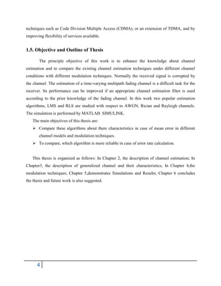
Figure-2.1: General channel estimation procedure[5]
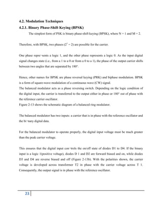
Channel estimation is based on the training sequence of bits and which is unique for a
certain transmitter and which is repeated in every transmitted burst. The channel estimator gives
the knowledge on the channel impulse response (CIR) to the detector and it estimates separately
the CIR for each burst by exploiting transmitted bits and corresponding received bits. Signal
detectors must have knowledge concerning the channel impulse response (CIR) of the radio link
with known transmitted sequences, which can be done by a separate channel estimator. The
modulated corrupted signal from the channel has to be undergoing the channel estimation using
LMS, MLSE, MMSE, RMS etc before the demodulation takes place at the receiver side[7]. The
channel estimator is shown in figure 2.2.
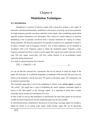
Error
Signal
e(n)
Actual
Received Signal
Channel
Estimated
Channel
Model
Estimation Algorithm
+
Estimated
Signal
)(ˆ nY
)(nY
Transmitted sequence
+
-
)(nx](https://image.slidesharecdn.com/58bf77a4-8f3b-4af1-a99b-cbcbac6c2b91-151202190833-lva1-app6891/85/part-2-Book-6-320.jpg)
![7
Figure 2.2 : The block diagram of the channel estimator [7]
A channel estimate is only a mathematical estimation of what is truly happening in nature.
Aim of any channel estimation procedure:
Minimize some sort of criteria, e.g. MSE.
Utilize as little computational resources as possible allowing easier implementation.
Why Channel Estimation?
Allows the receiver to approximate the effect of the channel on the signal.
The channel estimate is essential for removing inter symbol interference, noise rejection
techniques etc.
Also used in diversity combining, ML detection, angle of arrival estimation etc.
2.2. Channel Estimation Techniques
A wideband radio channel is normally frequency selective and time variant.For an
OFDM mobile communication system, the channel transfer function at different subcarriers
appears unequal in both frequency and time domains. Therefore, a dynamic estimation of the
channel is necessary. Pilot-based approaches are widely used to estimate the channel properties](https://image.slidesharecdn.com/58bf77a4-8f3b-4af1-a99b-cbcbac6c2b91-151202190833-lva1-app6891/85/part-2-Book-7-320.jpg)
![8
and correct the received signal. In this chapter we have investigated two types of pilot
arrangements[3].
Figure-2.3 Block type pilot arrangement[3] Figure-2.4 Comb type pilot arrangement[3]
The first kind of pilot arrangement shown in Figure 2.3 is denoted as block-type pilot
arrangement. The pilot signal assigned to a particular OFDM block, which is sent periodically in
time-domain. This type of pilot arrangement is especially suitable for slow-fading radio
channels. Because the training block contains all pilots, channel interpolation in frequency
domain is not required. Therefore, this type of pilot arrangement is relatively insensitive to
frequency selectivity. The second kind of pilot arrangement shown in Figure 2.4 is denoted as
comb-type pilot arrangement. The pilot arrangements are uniformly distributed within each
OFDM block. Assuming that the payloads of pilot arrangements are the same, the comb-type
pilot arrangement has a higher re-transmission rate. Thus the comb-type pilot arrangement
system is provides better resistance to fast-fading channels. Since only some sub-carriers contain
the pilot signal, the channel response of non-pilot sub-carriers will be estimated by interpolating
neighboring pilot sub-channels. Thus the comb-type pilot arrangement is sensitive to frequency
selectivity when comparing to the block-type pilot arrangement system.
2.2.1 Channel Estimation Based on Block-Type Pilot Arrangement
In block-type pilot based channel estimation, OFDM channel estimation symbols are transmitted
periodically, in which all sub-carriers are used as pilots. If the channel is constant during the
block, there will be no channel estimation error since the pilots are sent at all carriers. The](https://image.slidesharecdn.com/58bf77a4-8f3b-4af1-a99b-cbcbac6c2b91-151202190833-lva1-app6891/85/part-2-Book-8-320.jpg)
![9
estimation can be performed by using either LSE or MMSE .If inter symbol interference is
eliminated by the guard interval, we write in matrix notation[3]:
Y=XFh+ W
= XH +W ……………………….2.1
2.2.2 Channel Estimation Based on Comb-Type Pilot Arrangement
In comb-type based channel estimation, the Np pilot signals are uniformly inserted
into X(k) according to following equation:
……………….2.2
L = number of carriers/Np
xp(m) is the mth pilot carrier value.
We define {Hp(k) k = 0, 1, . . . Np} as the frequency response of the channel at pilot sub-carriers.
The estimate of the channel at pilot sub-carriers based on LS estimation is given by:
…………………..2.3
Yp(k) and Xp(k) are output and input at the k th pilot sub-carrier respectively[3].](https://image.slidesharecdn.com/58bf77a4-8f3b-4af1-a99b-cbcbac6c2b91-151202190833-lva1-app6891/85/part-2-Book-9-320.jpg)
![10
2.3. Channel Estimation Algorithm
Mainly two types of adaptive algorithms are used in channel estimation purpose. The
algorithms are Least-Mean Square (LMS) & Recursive Least-Squares (RLS).
2.3.1 Least-Mean Square (LMS) Algorithm
LMS algorithm uses the estimates of the gradient vector from the available data.
LMS incorporates an iterative procedure that makes successive corrections to the
weight vector in the direction of the negative of the gradient vector which eventually
leads to the minimum mean square error. Compared to other algorithms LMS
algorithm is relatively simple.
Input: A random process x(n);
FIR filter of weight: (w0, w1…wN-1);
Filter output:Y(n)=wT
x(n) ;
Error signal:d(n)-y(n) ;Where d(n) is the desired output.
From the method of steepest descent, the weight vector equation is given by:
W (n) = W (n) +1/ 2[-(E{e2
(n)}] ………………………..2.4
Where μ is the step-size parameter and controls the convergence characteristics of the LMS
algorithm[4]. In the method of steepest descent the biggest problem is the computation involved
in finding the values r and R matrices in real time. The LMS algorithm on the other hand
simplifies this by using the instantaneous values of covariance matrices r and R instead of their
actual values i.e.
…………………………………….2.5
……………………………………..2.6
Therefore the weight update can be given by the following equation:
w(n +1) = w(n) + x(n)[d *
(n) - xT
(n)w(n)] = w(n) + x(n)e*
(n) ………….2.7
R(n) = x(n)xT
(n)
r(n) = d *
(n)x(n)](https://image.slidesharecdn.com/58bf77a4-8f3b-4af1-a99b-cbcbac6c2b91-151202190833-lva1-app6891/85/part-2-Book-10-320.jpg)
![11
………………………….2.8
…………………………2.9
Equation number (2.6) & (2.9) are respectively known as weight update & filtering operation
equation.
2.3.2 Recursive Least Square (RLS) Algorithm
The Recursive least squares (RLS) adaptive filter is an algorithm which recursively finds the
filter coefficients that minimize a weighted linear least squares cost function relating to the input
signals. This is in contrast to other algorithms such as the least mean squares (LMS) that aim to
reduce the mean square error[8][9].
The RLS algorithm for a p-th order RLS filter can be summarized as, Parameters:
p = Filter order
= Forgetting factor
= Value of initialize P(0)
Initialization: wn = 0
P(0) = -1
I Where I is the (p+1)-by-(p+1) identity matrix Computation: For n= 0,1,2,…….
Then the weight update can be given by the following equation:
w(n) = w(n -1) +(n)g(n) ……………………………..2.10
e(n) = d(n) - y(n) [n = 0 to final ]
Y (n) = wT
(n)x(n)](https://image.slidesharecdn.com/58bf77a4-8f3b-4af1-a99b-cbcbac6c2b91-151202190833-lva1-app6891/85/part-2-Book-11-320.jpg)
![12
Chapter-3
Communication Channel
3.1. Introduction
There are three basic types of channels considered for this work. The vehicle-to-vehicle
(V2V) channels estimation are compared with cellular channels. Performance of three channels,
viz., AWGN, Rayleigh Fading Channel, Rician Fading Channel in V2V communication
environment is evaluated through simulation.
Multipath fading is a significant problem in communications. In a fading channel, signals
experience fades (i.e., they fluctuate in their strength). When the signal power drops
significantly, the channel is said to be in a fade. This gives rise to high bit error rates (BER).
3.2. Channel Models
3.2.1. AWGN Channel:
An Additive white Gaussian noise (AWGN) channel adds white Gaussian noise to the
signal, when the signal passes through it. In this channel model the only impairment to
communication is a linear addition of wideband or white noise with a constant spectral density
and a Gaussian distribution of amplitude. Fading, frequency selectivity, interference, nonlinearity
or dispersion are not the part of AWGN model. It generates simple and tractable mathematical
models. Those models are useful for gaining insight into the underlying behavior of a system
before these other phenomena are considered.
In case for many satellite and deep space communication links, the AWGN model is very good.
This model is not useful for most terrestrial links because of multipath, terrain blocking,
interference, etc. However AWGN is used to simulate background noise of the channel under
study, in addition to multipath, terrain blocking, interference, ground clutter, etc[8][10].](https://image.slidesharecdn.com/58bf77a4-8f3b-4af1-a99b-cbcbac6c2b91-151202190833-lva1-app6891/85/part-2-Book-12-320.jpg)
![13
Figure-3.1: AWGN channels at least one existing LOS[8].
The AWGN channel is represented by a series of outputs Si at discrete time event index i. Si is
the sum of the input Ri and noise, Qi, where Qi is independent and identically-distributed and
drawn from a zero-mean normal distribution with variance n (the noise). The Qi are further
assumed to not be correlated with the Xi.
Qi ≈N(0.n) Si =Ri + Qi …………………………….3.1
The channel capacity C for the AWGN channel is given by:
C=1/2 log(1+𝑃/𝑛) ……………………………3.2
Where P = maximum channel power.
3.2.2 Rician Fading Channel:
Rician fading is a stochastic model. It is used for radio propagation anomaly caused by
partial cancellation of a radio signal by itself, the signal arrives at the receiver by several
different paths (hence exhibiting multipath interference), and at least one of the paths is changing
(lengthening or shortening). Rician fading model applicable where one dominant propagation
along a line of sight between the transmitter and receiver; typically a line of sight (LOS) signal is
much stronger than the others signal. In Rician fading, the amplitude gain is characterized by a
Rician distribution[8][11].](https://image.slidesharecdn.com/58bf77a4-8f3b-4af1-a99b-cbcbac6c2b91-151202190833-lva1-app6891/85/part-2-Book-13-320.jpg)
![14
K and Ω are the two parameters of Rician fading channel. K is the ratio between the
power in the direct path and the power in the other, scattered, paths. Ω is the power in the direct
path. The received signal amplitude (not the power of the received signal) R is then Rice
distributed.
……………………3.3
Figure-3.2: Rician Fading Channel with existing one LOS[8].
3.2.3. Rayleigh Fading Channel:
Rayleigh fading channel is a statistical model. It assumes the magnitude of a signal. This
model is used for the effect of a propagation environment on a radio signal, such as that used by
wireless devices.
When the signal has passed through such a transmission medium (communications channel) will
vary randomly, or fade, according to a Rayleigh distribution — the radial component of the sum
of two uncorrelated Gaussian random variables.](https://image.slidesharecdn.com/58bf77a4-8f3b-4af1-a99b-cbcbac6c2b91-151202190833-lva1-app6891/85/part-2-Book-14-320.jpg)
![15
Rayleigh fading is viewed as a sensible model for tropospheric and ionospheric signal
propagation and it is used for the effect of heavily built-up urban environments on radio signals.
If there is no dominant propagation along a line of sight between the transmitter and receiver,
there Rayleigh fading model is applicable. In case of one dominant line of sight, Rician fading
may be more applicable.
Rayleigh fading is a sensible model when there are many objects in the environment that scatter
the radio signal before it arrives at the receiver. If there is sufficiently much scatter, the channel
impulse response will be well-modeled as a Gaussian process irrespective of the distribution of
the individual components. Transmitted signal of Rayleigh fading model is affected by
multipath. If there is no dominant component to the scatter, then such a process will have zero
mean and phase evenly distributed between 0 and 2π radians. The envelope of the channel
response will therefore be Rayleigh distributed[8][12].
Calling this random variable R, it will have a probability density function:
PR(r) = r>=0 …………………………….3.4
Where 𝜴 = E(R2
).
Figure-3.3: Rayleigh Fading Channel with no existing LOS[8].](https://image.slidesharecdn.com/58bf77a4-8f3b-4af1-a99b-cbcbac6c2b91-151202190833-lva1-app6891/85/part-2-Book-15-320.jpg)
![16
3.3. Channel in Intelligent Transport Systems (ITS)
The development of the future V2V and Vehicle-to- Infrastructure (V2I) communications
systems imposes strong radio channel management challenges due to their decentralized nature
and the strict Quality of Service (QoS) requirements of traffic safety applications[8].
In ITS channel, scattering can occur around both the TX and the RX, on the other hand
base station is usually free of scatter.
The distance over which communications can take place is much smaller in ITS channels
(< 100 m) than in typical cellular scenarios (~ 1 km).
In cellular communication only Tx or Rx is moving, for ITS both are moving.
ITS operates most high carrier frequency (5.8- 5.9GHz), whereas Cellular
communication operates mostly 700-2400MHz.
The ITS ad-hoc communications are peer-to-peer communications, thus the transmitter
and receiver are at the same height and the same environment. On the other hand in
cellular communication the base station is high above the street level and the mobile
station is at the street level. Thus the dominant propagation mechanisms of the multipath
components are different.
3.4. Propagation Characteristics of Channels
For an ideal radio channel, the received signal would consist of only a single directpath
signal, which would be a perfect reconstruction of the transmitted signal.However in a real
channel, the signal is modified during transmission in the channel. The received signal consists
of a combination of attenuated, reflected, refracted, and diffracted replicas of the transmitted
signal. On top of all this, the channel adds noise to the signal and can cause a shift in the carrier
frequency if the transmitter or receiver is moving (Doppler effect). Understanding of these
effects on the signal is important because the performance of a radio system is dependent on the
radio channel characteristics[3].](https://image.slidesharecdn.com/58bf77a4-8f3b-4af1-a99b-cbcbac6c2b91-151202190833-lva1-app6891/85/part-2-Book-16-320.jpg)
![17
3.4.1. Attenuation
Attenuation is the drop in the signal power when transmitting from one point to the
another. It can be caused by the transmission path length, obstructions in the signal path and
multipath effects. Any objects, which obstruct the line of sight signal from the transmitter to the
receiver, can cause attenuation. Shadowing of the signal can occur whenever there is an
obstruction between the transmitter and receiver. It is generally caused by buildings and hills,
and is the most important environmental attenuation factor.
Figure-3.4: Attenuation of signal[3].
Shadowing is most severe in heavily built up areas, due to the shadowing from buildings.
However, hills can cause a large problem due to the large shadow they produce. Radio signals
diffract off the boundaries of obstructions, thus preventing total shadowing of the signals behind
hills and buildings. However, the amount of diffraction is dependent on the radio frequency used,
with low frequencies diffracting more than high frequency signals. Thus, high frequency signals,
especially, Ultra High Frequencies (UHF), and microwave signals require line of sight for
adequate signal strength. To overcome the problem of shadowing, transmitters are usually
elevated as high as possible to minimise the number of obstructions[3].](https://image.slidesharecdn.com/58bf77a4-8f3b-4af1-a99b-cbcbac6c2b91-151202190833-lva1-app6891/85/part-2-Book-17-320.jpg)
![18
3.4.2 Frequency Selective Fading
In any radio transmission, the channel spectral response is not flat. It has dips or fades in
the response due to reflections causing cancellation of certain frequencies at the receiver.
Reflections off near-by objects (e.g. ground, buildings, trees, etc) can lead to multipath signals of
similar signal power as the direct signal. This can result in deep nulls in the received signal
power due to destructive interference.For narrow bandwidth transmissions if the null in the
frequency response occurs at the transmission frequency then the entire signal can be lost. This
can be partly overcome in two ways. By transmitting a wide bandwidth signal or spread
spectrum as CDMA, any dips in the spectrum only result in a small loss of signal power, rather
than a complete loss. Another method is to split the transmission up into many small bandwidth
carriers, as is done in a COFDM/OFDM transmission. The original signal is spread over a wide
bandwidth and thus, any nulls in the spectrum are unlikely to occur at all of the carrier
frequencies. This will result in only some of the carriers being lost, rather than the entire signal.
The information in the lost carriers can be recovered provided enough forward error corrections
is sent[3].
3.4.3 Delay Spread
The received radio signal from a transmitter consists of typically a direct signal,plus
reflections of object such as buildings, mountings, and other structures. The reflected signals
arrive at a later time than the direct signal because of the extra path length, giving rise to a
slightly different arrival time of the transmitted pulse, thus spreading the received energy. Delay
spread is the time spread between the arrival of the first and last multipath signal seen by the
receiver. In a digital system, the delay spread can lead to inter-symbol interference. This is due to
the delayed multipath signal overlapping with the following symbols. This can cause significant
errors in high bit rate systems, especially when using time division multiplexing (TDMA). As the
transmitted bit rate is increased the amount of inter symbol interference also increases. The effect
starts to become very significant when the delay spread is greater than ~50% of the bit time[3].](https://image.slidesharecdn.com/58bf77a4-8f3b-4af1-a99b-cbcbac6c2b91-151202190833-lva1-app6891/85/part-2-Book-18-320.jpg)
![19
Figure-3.5: Delay spread[3].
3.4.4. Doppler Shift
When a wave source and a receiver are moving relative to one another the frequency of
the received signal will not be the same as the source. When they are moving toward each other
the frequency of the received signal is higher than the source, and when they are approaching
each other the frequency decreases. This is called the Doppler’s effect. An example of this is the
change of pitch in a car’s horn as it approaches then passes by. This effect becomes important
when developing mobile radio systems.
The amount the frequency changes due to the Doppler effect depends on the relative motion
between the source and receiver and on the speed of propagation of the wave. The Doppler shift
in frequency can be written
Δ f ≈ +- f 0 v/c ……………………………….3.5
where f is the change in frequency of the source seen at the receiver, fo is the frequency of the
source, v is the speed difference between the source and transmitter, and c is the speed of light.
Doppler shift can cause significant problems if the transmission technique is sensitive to carrier
frequency offsets or the relative speed is higher, which is the case for OFDM. If we consider
now a link between to cars moving in opposite directions, each one with a speed of 80 km/hr, the
Doppler shift will be double[3].](https://image.slidesharecdn.com/58bf77a4-8f3b-4af1-a99b-cbcbac6c2b91-151202190833-lva1-app6891/85/part-2-Book-19-320.jpg)
![26
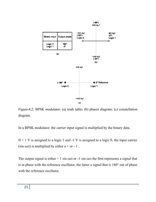
Each time the input logic condition changes, the output phase changes.
Mathematically, the output of a BPSK modulator is proportional to
BPSK output = [sin (2πfat)] x [sin (2πfct)] (2.20)
where
fa = maximum fundamental frequency of binary input (hertz)
fc = reference carrier frequency (hertz)
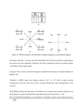
4.2.2. Quaternary Phase-Shift Keying (QPSK)
QPSK is an M-ary encoding scheme where N = 2 and M= 4 (hence, the name
"quaternary" meaning "4"). A QPSK modulator is a binary (base 2) signal, to produce four
different input combinations,: 00, 01, 10, and 11.
Therefore, with QPSK, the binary input data are combined into groups of two bits, called dibits.
In the modulator, each dibit code generates one of the four possible output phases (+45°,
+135°, -45°, and -135°).
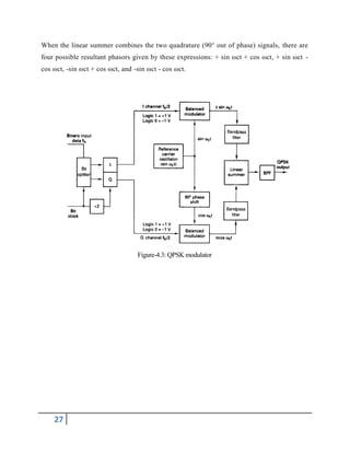
A block diagram of a QPSK modulator is shown in Figure 4.3. Two bits (a dibit) are
clocked into the bit splitter. After both bits have been serially inputted, they are
simultaneously parallel outputted.
The I bit modulates a carrier that is in phase with the reference oscillator (hence the name
"I" for "in phase" channel), and the Q bit modulate, a carrier that is 90° out of phase.
For a logic 1 = + 1 V and a logic 0= - 1 V, two phases are possible at the output of the I
balanced modulator (+sin ωct and - sin ωct), and two phases are possible at the output of the
Q balanced modulator (+cos ωct), and (-cos ωct).](https://image.slidesharecdn.com/58bf77a4-8f3b-4af1-a99b-cbcbac6c2b91-151202190833-lva1-app6891/85/part-2-Book-26-320.jpg)
![41
REFERENCES
[1].Haykin, S. (1996), ―‖Adaptive Filter Theory, 3/e‖, Prentice Hall.
[2].S.Dhar, R.Bera, R.B. Giri, S.Anand, D.Nath, S.Kumar (2011), ―‖An Overview of V2V
Communication Channel Modeling”, in proceedings of ISDMISC’11, 12-14 April, 2011,
Sikkim, India.
[3].Sarada Prasanna Dash, Bikash Kumar Dora –―Channel estimation in multicarrier
communication systems‖.
[4].Shetty k.k. ―LEAST MEAN SQUARE ALGORITHM.
[5].Rupul Safaya -A Multipath Channel Estimation Algorithm using the Kalman Filter.
[6].Jones et al. ―‖Adaptive Filtering: LMS Algorithm‖-02.06.2005 16:10 filterdesign
exercise in matlab.
[7].Markku Pukkila, Nokia Research –“CenterChannel Estimation Modeling”.
[8].Tirthankar Paul, Priyabrata karmakar, Sourav Dhar ―Comparative Study of Channel
Estimation Algorithms under Different Channel Scenario” ― International Journal of
Computer Applications (0975 – 8887) Volume 34– No.7, November 2011
[9].RLS online available at: http://en.wikipedia.org/wiki/ Recursive_least_squares_filter
[10]. Additive white Gaussian noise online available at:
http://en.wikipedia.org/wiki/Additive_white_Gaussian_noise
[11]. Rician fading online available at: http://en.wikipedia.org/ wiki/Rician_fading
[12]. Rayleigh fading online available at: http://en.wikipedia. org/wiki/Rayleigh_fading](https://image.slidesharecdn.com/58bf77a4-8f3b-4af1-a99b-cbcbac6c2b91-151202190833-lva1-app6891/85/part-2-Book-41-320.jpg)

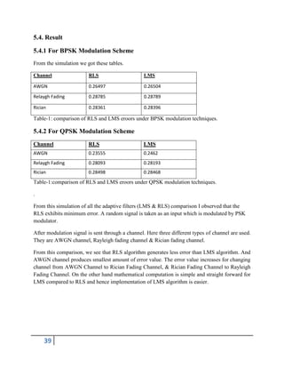
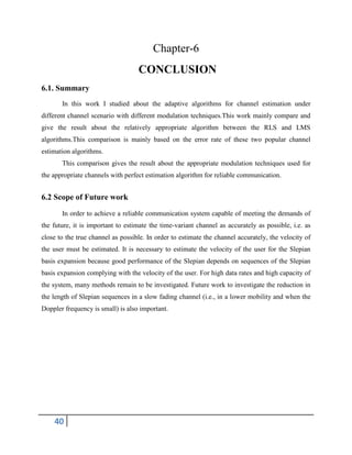
The document discusses channel estimation techniques for wireless communication systems. It describes that channel estimation is important for mobile wireless networks as the channel changes over time due to movement. It summarizes that channel estimation algorithms allow the receiver to approximate the time-varying channel impulse response. The document then compares two popular channel estimation algorithms - LMS and RLS. LMS uses estimates of the gradient vector to iteratively minimize the mean square error, while RLS recursively finds filter coefficients to minimize a weighted linear least squares cost function.


![[Signals and Communication Technology ] Joachim Speidel - Introduction to Dig...](https://cdn.slidesharecdn.com/ss_thumbnails/signalsandcommunicationtechnologyjoachimspeidel-introductiontodigitalcommunications2019springer10-230125181149-9706aeb5-thumbnail.jpg?width=640&height=640&fit=bounds)


