Downloaded 199 times


![8
This Week: A Packet Walkthrough on the M, MX, and T Series
Figure 1.2
VLANs and Logical Connections Between the Routers
Inline Packet Captures
Capturing traffic in the wire, by mirroring packets at switch X towards server H, is a
cornerstone of this chapter.
Let’s start the packet capture at H:
[root@H ~]# tcpdump -nv -s 1500 -i bce1
tcpdump: listening on bce1, link-type EN10MB (Ethernet), capture size 1500 bytes
You can see this capture shows all traffic in the monitored VLANs, including routing
protocol exchanges and transit data traffic. There are several ways to successfully find
the packets involved in your ping:
„„ Decode the capture in real-time with a graphical utility like Wireshark (http://
www.wireshark.org/) and filter the view. Alternatively, you can save the capture
to a file and view it offline.
„„ Just let the capture run on the terminal and do a pattern search in the scroll
buffer. You may have to clear the buffer often so that you can easily find the last
flow. This can either be very easy, or a nightmare, depending on the terminal
software.
„„ Remove the -v option so that only one line is displayed per packet. You will find
the packets more easily, but obviously lose some details.
„„ Use tcpdump filtering expressions. This is not guaranteed to work, as the
mirrored packets have a VLAN tag that doesn’t match H’s interface.](https://image.slidesharecdn.com/packetwalkthrough-131115184203-phpapp02/85/Packet-walkthrough-10-320.jpg)

![10
This Week: A Packet Walkthrough on the M, MX, and T Series
verbose output suppressed, use <detail> or <extensive> for full protocol decode
Address resolution is OFF.
Listening on ge-1/0/0.101, capture size 2000 bytes
<timestamp> Out arp who-has 10.1.1.1 tell 10.1.1.2
<timestamp> Out arp who-has 10.1.1.1 tell 10.1.1.2
[...]
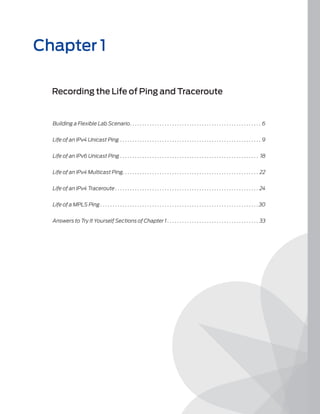
So, CE1 is generating ARP requests, but it never receives an ARP reply back. The
result is that CE1 cannot resolve the MAC address of 10.1.1.1, the next hop for IPv4
packets destined to 10.2.2.2.
Hence, even though you successfully configured a static route at CE1 towards 10/8, it
remains in a hold state at the forwarding table:
user@PE1> show route 10.2.2.2 table CE1
CE1.inet.0: 3 destinations, 3 routes (3 active, 0 holddown, 0 hidden)
+ = Active Route, - = Last Active, * = Both
10.0.0.0/8
*[Static/5] 00:09:39
> to 10.1.1.1 via ge-1/0/0.101
user@PE1> show route forwarding-table destination 10.2.2.2 table CE1
Routing table: CE1.inet
Internet:
Destination
Type RtRef Next hop
Type Index NhRef Netif
10.0.0.0/8
user
0 10.1.1.1
hold 532
3 ge-1/0/0.101
user@PE1> show arp vpn CE1
/* Starting with Junos 11.1, you can use the interface option too */
user@PE1>
For this same reason, the local IP address of VRF1 is also not reachable from CE1:
user@PE1> ping 10.1.1.1 routing-instance CE1 count 1
PING 10.1.1.1 (10.1.1.1): 56 data bytes
--- 10.1.1.1 ping statistics --1 packets transmitted, 0 packets received, 100% packet loss
user@PE1> show route forwarding-table destination 10.1.1.1 table CE1
Routing table: CE1.inet
Internet:
Destination
Type RtRef Next hop
Type Index NhRef Netif
10.1.1.1/32
dest
0 10.1.1.1
hold 582
3 ge-1/0/0.101
Before turning off the ARP filtering at the switch X, let’s try to see what can be done
when ARP resolution is failing. One option is to configure static ARP resolution at
the [edit interfaces <...> family inet address <...> arp] hierarchy, but let’s use
a different approach in which we also need to know the MAC address of the local
interface at VRF1:
user@PE1> show interfaces ge-1/0/1 | match hardware
Current address: 5c:5e:ab:0a:c3:61, Hardware address: 5c:5e:ab:0a:c3:61
Now, the following ping command allows you to specify the destination MAC
address while bypassing the forwarding table lookup:
user@PE1> ping 10.1.1.1 bypass-routing interface ge-1/0/0.101 mac-address 5c:5e:ab:0a:c3:61 count 1](https://image.slidesharecdn.com/packetwalkthrough-131115184203-phpapp02/85/Packet-walkthrough-12-320.jpg)
![Chapter 1: Recording the Life of Ping and Traceroute
11
PING 10.1.1.1 (10.1.1.1): 56 data bytes
--- 10.1.1.1 ping statistics --1 packets transmitted, 0 packets received, 100% packet loss
NOTE The mac-address ping option has been supported since Junos OS 11.1. It’s mutually
exclusive with the routing-instance option.
Although ping still fails, the echo request is sent this time. You can see it in Capture
1.1, that was taken at H:
[timestamp] IP (tos 0x0, ttl 64, id 60312, offset 0, flags [none], proto ICMP (1), length 84)
10.1.1.2 > 10.1.1.1: ICMP echo request, id 3526, seq 0, length 64
TRY THIS
Increase the packet count value. Unlike the IPv4 ID, the ICMPv4 ID value remains
constant in all the same-ping packets and identifies the ping flow. The sequence
number increases one by one.
The ping command originates IP packets with IP protocol #1, corresponding to
ICMPv4. It’s also interesting to see the packet at the VRF1 end, by running tcpdump
in a parallel session at PE1, while you launch ping again:
user@PE1> monitor traffic interface ge-1/0/1.101 no-resolve size 2000
verbose output suppressed, use <detail> or <extensive> for full protocol decode
Address resolution is OFF.
Listening on ge-1/0/1.101, capture size 2000 bytes
<timestamp>
<timestamp>
<timestamp>
<timestamp>
<timestamp>
<timestamp>
In
Out
Out
Out
Out
Out
IP 10.1.1.2
arp who-has
arp who-has
arp who-has
arp who-has
arp who-has
> 10.1.1.1: ICMP echo request, id 3530, seq 0, length 64
10.1.1.2 tell 10.1.1.1
10.1.1.2 tell 10.1.1.1
10.1.1.2 tell 10.1.1.1
10.1.1.2 tell 10.1.1.1
10.1.1.2 tell 10.1.1.1
VRF1 at PE1 cannot resolve the MAC address associated to 10.1.1.2, hence ping
fails. There is an interesting difference in behavior between CE1 and VRF1. While
CE1 sends ARP requests periodically (every ~15 seconds), VRF1 only does it if
triggered by a ping command. Can you spot the reason? Actually, CE1 has a static
route pointing to 10.1.1.1 as next hop: as long as it is in hold state, CE1 will keep
trying to resolve it over and over again.
Now it’s time to remove the ARP filter from the switch. While keeping the packet
capture active at H, execute:
user@X>
user@X#
user@X#
user@X#
configure
delete interfaces ge-0/0/11 unit 0 family ethernet-switching filter
delete interfaces ge-0/0/14 unit 0 family ethernet-switching filter
commit and-quit
The Junos OS kernel keeps trying to complete the pending ARP resolutions for the
next hops in its forwarding table. At some point you should see in Capture 1.2 the
ARP reply, as shown in Figure 1.3:
<timestamp> ARP, Ethernet (len 6), IPv4 (len 4), Request who-has 10.1.1.1 tell 10.1.1.2, length 42
---------------------------------------------------------------------------------<timestamp> ARP, Ethernet (len 6), IPv4 (len 4), Reply 10.1.1.1 is-at 5c:5e:ab:0a:c3:61, length 42](https://image.slidesharecdn.com/packetwalkthrough-131115184203-phpapp02/85/Packet-walkthrough-13-320.jpg)

![Chapter 1: Recording the Life of Ping and Traceroute
13
And capture 1.3 at H shows both the one-hop ICMPv4 request and the reply:
<timestamp> IP (tos 0x0, ttl 64, id 7523, offset 0, flags [none], proto ICMP (1), length 84)
10.1.1.2 > 10.1.1.1: ICMP echo request, id 3546, seq 0, length 64
---------------------------------------------------------------------------------<timestamp> IP (tos 0x0, ttl 64, id 7526, offset 0, flags [none], proto ICMP (1), length 84)
10.1.1.1 > 10.1.1.2: ICMP echo reply, id 3546, seq 0, length 64
Taking the ICMPv4 Echo Request to its Destination
Now that CE1 can finally send the packet to the next hop, check out what comes
next:
user@PE1> show route forwarding-table destination 10.2.2.2 table CE1
Routing table: CE1.inet
Internet:
Destination
Type RtRef Next hop
Type Index NhRef Netif
10.0.0.0/8
user
0 5c:5e:ab:a:c3:61 ucst 532
3 ge-1/0/0.101
user@PE1> ping 10.2.2.2 routing-instance CE1 count 1
PING 10.2.2.2 (10.2.2.2): 56 data bytes
36 bytes from 10.1.1.1: Destination Net Unreachable
Vr HL TOS Len ID Flg off TTL Pro cks
Src
Dst
4 5 00 0054 231a 0 0000 40 01 4089 10.1.1.2 10.2.2.2
--- 10.2.2.2 ping statistics --1 packets transmitted, 0 packets received, 100% packet loss
TIP
If you configured a name-server, PE1 tries to resolve 10.1.1.1, 10.1.1.2, and 10.2.2.2
into hostnames. If the server is not responsive, you can avoid significant delay with
the no-resolve ping option.
So ping still fails because PE1 does not have a route to the destination yet. Let’s look
at the ICMPv4 packets in Capture 1.4, taken at H:
[timestamp] IP (tos 0x0, ttl 64, id 13549, offset 0, flags [none], proto ICMP (1), length 84)
10.1.1.2 > 10.2.2.2: ICMP echo request, id 3559, seq 0, length 64
---------------------------------------------------------------------------------[timestamp] IP (tos 0x0, ttl 255, id 0, offset 0, flags [none], proto ICMP (1), length 56)
10.1.1.1 > 10.1.1.2: ICMP net 10.2.2.2 unreachable, length 36
IP (tos 0x0, ttl 64, id 13549, offset 0, flags [none], proto ICMP (1), length 84)
10.1.1.2 > 10.2.2.2: ICMP echo request, id 3559, seq 0, length 64
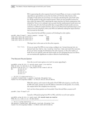
As you can see, the ping command originates IP packets with IP protocol #1, corresponding to ICMPv4. The ICMP protocol is also used to report errors, such as the
one indicating net unreachable. Figure 1.4 shows the complete message exchange.
Look closely at the ICMPv4 header with a graphical analyzer like Wireshark, then
match the echo request and net unreachable messages to Table 1.1 near the end of this
chapter.](https://image.slidesharecdn.com/packetwalkthrough-131115184203-phpapp02/85/Packet-walkthrough-15-320.jpg)

![Chapter 1: Recording the Life of Ping and Traceroute
15
Verify at PE1 and PE2 that the BGP session is established:
user@PE1> show bgp summary
Groups: 1 Peers: 1 Down peers: 0
Table
Tot Paths Act Paths Suppressed
inet.0
0
0
0
bgp.l3vpn.0
1
1
0
Peer
AS
InPkt
OutPkt
Accepted/Damped...
10.111.2.2
65000
41
33
bgp.l3vpn.0: 1/1/1/0
VRF1.inet.0: 1/1/1/0
History Damp State
Pending
0
0
0
0
0
0
OutQ Flaps Last Up/Dwn State|#Active/Received/
0
2
6:41 Establ
Send one more single-packet ping:
user@PE1> ping 10.2.2.2 routing-instance CE1 count 1
PING 10.2.2.2 (10.2.2.2): 56 data bytes
--- 10.2.2.2 ping statistics --1 packets transmitted, 0 packets received, 100% packet loss
Now the capture 1.5 at H shows the same ICMPv4 echo request packet four times,
one at each segment of its trip from CE1 to CE2. What follows is just one single
packet at different stages of its life through the network:
[timestamp] IP (tos 0x0, ttl 64, id 40308, offset 0, flags [none], proto ICMP (1), length 84)
10.1.1.2 > 10.2.2.2: ICMP echo request, id 3649, seq 0, length 64
---------------------------------------------------------------------------------[timestamp] MPLS (label 299840, exp 0, ttl 63)
(label 16, exp 0, [S], ttl 63)
IP (tos 0x0, ttl 63, id 40308, offset 0, flags [none], proto ICMP (1), length 84)
10.1.1.2 > 10.2.2.2: ICMP echo request, id 3649, seq 0, length 64
---------------------------------------------------------------------------------[timestamp] MPLS (label 16, exp 0, [S], ttl 62)
IP (tos 0x0, ttl 63, id 40308, offset 0, flags [none], proto ICMP (1), length 84)
10.1.1.2 > 10.2.2.2: ICMP echo request, id 3649, seq 0, length 64
---------------------------------------------------------------------------------[timestamp] IP (tos 0x0, ttl 61, id 40308, offset 0, flags [none], proto ICMP (1), length 84)
10.1.1.2 > 10.2.2.2: ICMP echo request, id 3649, seq 0, length 64
ALERT!
This is just one packet! The proof is in the IPv4 header ID, which remains the same as
it travels along the router hops. In addition, as you will see in Chapter 4, when an
IPv4 packet is fragmented somewhere in the path, all the resulting fragments also
keep the original IPv4 ID.
Figure 1.5 provides detail of the different encapsulations at each stage of the packet.
MPLS labels may have different values in your scenario.](https://image.slidesharecdn.com/packetwalkthrough-131115184203-phpapp02/85/Packet-walkthrough-17-320.jpg)

![Chapter 1: Recording the Life of Ping and Traceroute
17
If you are puzzled at this point, that’s okay! The filter was applied at lo0.0, but lo0.0 is
in the master instance inet.0, so why did it affect traffic addressed to CE2 at all? Well,
in Junos, if a routing instance (in this case, CE2) has no local lo0 unit, all its input
control traffic is evaluated by the master instance’s lo0 filter.
TRY THIS
Put the lo0.0 filter back in place, create lo0.1, and associate it to routing-instance
CE2. The end-to-end ping should still succeed!
The ICMPv4 echo reply now shows up once at each of the four network segments in
Capture 1.6 at H, as illustrated in Figure 1.6:
[timestamp] IP (tos 0x0, ttl 64, id 40242, offset 0, flags [none], proto ICMP (1), length 84)
10.2.2.2 > 10.1.1.2: ICMP echo reply, id 3691, seq 0, length 64
---------------------------------------------------------------------------------[timestamp] MPLS (label 299872, exp 0, ttl 63)
(label 16, exp 0, [S], ttl 63)
IP (tos 0x0, ttl 63, id 40242, offset 0, flags [none], proto ICMP (1), length 84)
10.2.2.2 > 10.1.1.2: ICMP echo reply, id 3691, seq 0, length 64
---------------------------------------------------------------------------------[timestamp] MPLS (label 16, exp 0, [S], ttl 62)
IP (tos 0x0, ttl 63, id 40242, offset 0, flags [none], proto ICMP (1), length 84)
10.2.2.2 > 10.1.1.2: ICMP echo reply, id 3691, seq 0, length 64
---------------------------------------------------------------------------------[timestamp] IP (tos 0x0, ttl 61, id 40242, offset 0, flags [none], proto ICMP (1), length 84)
10.2.2.2 > 10.1.1.2: ICMP echo reply, id 3691, seq 0, length 64
Look closely at Capture 1.6 with a graphical analyzer like Wireshark, and start by
matching the echo reply message to Table 1.1.
The sequence number is 0 for the first packet of a ping flow, and it increments sequentially for the following packets (if the count is greater than 1 or not specified). In this
way, you can match an echo reply to the request that triggered it. What if you simultaneously execute the same ping command from different terminals? The ID inside the
ICMPv4 header (not to be mistaken for the IPv4 ID) is copied from the echo request
into the echo reply: in this way, the sender can differentiate several ping streams.
Figure 1.6
Life of an ICMPv4 Echo Reply from CE2 to CE1](https://image.slidesharecdn.com/packetwalkthrough-131115184203-phpapp02/85/Packet-walkthrough-19-320.jpg)
![18
This Week: A Packet Walkthrough on the M, MX, and T Series
This video camera assists you with analyzing any (ICMP is just one example)
protocol conversation in the complete forwarding path, including the endpoints as
well as the transit segments.
Life of an IPv6 Unicast Ping
There are many points in common between ICMPv6 and ICMPv4, but there are
differences, too. Let’s start with the IPv6-to-MAC address resolution.
Troubleshooting One-Hop IPv6 Connectivity
With the capture started at H, execute:
user@PE1> clear ipv6 neighbors
fc00::1:1
5c:5e:ab:0a:c3:61 deleted
[...]
And capture 1.7 at H shows (you can also see in Figure 1.7):
<timestamp> IP6 (hlim 255, next-header ICMPv6 (58) payload length: 32) fe80::5e5e:ab00:650a:c360 >
ff02::1:ff01:1: [icmp6 sum ok] ICMP6, neighbor solicitation, length 32, who has fc00::1:1
source link-address option (1), length 8 (1): 5c:5e:ab:0a:c3:60
---------------------------------------------------------------------------------<timestamp> IP6 (hlim 255, next-header ICMPv6 (58) payload length: 32) fe80::5e5e:ab00:650a:c361 >
fe80::5e5e:ab00:650a:c360: [icmp6 sum ok] ICMP6, neighbor advertisement, length 32, tgt is
fc00::1:1, Flags [router, solicited, override]
destination link-address option (2), length 8 (1): 5c:5e:ab:0a:c3:61
In the IPv6 world ICMPv6 is also used to achieve the same functionality as ARP in
IPv4, and this process is part of Neighbor Discovery (ND).
Figure 1.7
IPv6 Neighbor Discovery at the First Hop](https://image.slidesharecdn.com/packetwalkthrough-131115184203-phpapp02/85/Packet-walkthrough-20-320.jpg)
![Chapter 1: Recording the Life of Ping and Traceroute
REVIEW
19
Can you spot why the ND process to learn about fc00::1:1 MAC from CE1 restarts
immediately without any ping to trigger it? You already saw the answer in the
equivalent IPv4 scenario.
Look closely at the ICMP payload with a graphical analyzer like Wireshark, then
match the neighbor solicitations and advertisements to Table 1.1.
NOTE
The multicast destination IPv6 address ff02::1:ff01:1: is the Solicited-Node address
associated to fc00::1:1, according to RFC 429: IP Version 6 Addressing Architecture.
The associated MAC address is further constructed according to RFC 6085: Address
Mapping of IPv6 Multicast Packets on Ethernet. Finally, you can have a look at RFC
4861: Neighbor Discovery for IP Version 6 (IPv6).
As an exercise to complete the one-hop connectivity check, verify that ping
fc00::1:1 routing-instance CE1 count 1 succeeds at PE1, and interpret the capture.
ICMPv6 Echo Request and Reply Between CE1 and CE2
Try to ping from CE1 to CE2:
user@PE1> ping fc00::2:2 routing-instance CE1 count 1
PING6(56=40+8+8 bytes) fc00::1:2 --> fc00::2:2
64 bytes from fc00::1:1: No Route to Destination
Vr TC Flow Plen Nxt Hlim
6 00 00000 0010 3a 40
fc00::1:2->fc00::2:2
ICMP6: type = 128, code = 0
--- fc00::2:2 ping6 statistics --1 packets transmitted, 0 packets received, 100% packet loss
Check Capture 1.8 at H, illustrated in Figure 1.8:
<timestamp> IP6 (hlim 64, next-header ICMPv6 (58) payload length: 16) fc00::1:2 > fc00::2:2: [icmp6
sum ok] ICMP6, echo request, length 16, seq 0
---------------------------------------------------------------------------------<timestamp> IP6 (hlim 64, next-header ICMPv6 (58) payload length: 64) fc00::1:1 > fc00::1:2: [icmp6
sum ok] ICMP6, destination unreachable, length 64, unreachable route fc00::2:2](https://image.slidesharecdn.com/packetwalkthrough-131115184203-phpapp02/85/Packet-walkthrough-21-320.jpg)


![user@PE2>
user@PE2#
user@PE2#
user@PE2#
user@PE2#
user@PE2#
10.1.1.2
user@PE2#
Chapter 1: Recording the Life of Ping and Traceroute
23
configure
set protocols bgp group IBGP family inet-mvpn signaling
set routing-instances VRF2 protocols mvpn
set routing-instances VRF2 protocols pim interface all mode sparse
set routing-instances VRF2 routing-options multicast ssm-groups 239/8
set protocols igmp interface ge-1/0/1.102 version 3 static group 239.1.1.1 source
commit and-quit
Check that the PIM join state is magically propagated up to VRF1:
user@PE1> show pim join instance VRF1
Instance: PIM.VRF1 Family: INET
R = Rendezvous Point Tree, S = Sparse, W = Wildcard
Group: 239.1.1.1
Source: 10.1.1.2
Flags: sparse,spt
Upstream interface: ge-1/0/1.101
Instance: PIM.VRF1 Family: INET6
R = Rendezvous Point Tree, S = Sparse, W = Wildcard
MORE?
Puzzled? If you want a better understanding of the configuration above, have a look
at the This Week: Deploying BGP Multicast VPN, 2nd Edition book, available at
http://www.juniper.net/dayone.
Launch a multicast ping from CE1:
user@PE1> ping 239.1.1.1 routing-instance CE1 count 1
PING 239.1.1.1 (239.1.1.1): 56 data bytes
--- 239.1.1.1 ping statistics --1 packets transmitted, 0 packets received, 100% packet loss
Nothing in the packet capture, right? At this point it’s very common to start configuring IPv4 multicast protocols (PIM, IGMP) at CE1, but that is useless if you are
trying to simulate a multicast source, which is stateless. You just need a few more
ping options:
user@PE1> ping 239.1.1.1 interface ge-1/0/0.101 count 1
PING 239.1.1.1 (239.1.1.1): 56 data bytes
--- 239.1.1.1 ping statistics --1 packets transmitted, 0 packets received, 100% packet loss
Capture 1.10 shows an ICMPv4 packet that only survives one hop:
<timestamp> IP (tos 0x0, ttl 1, id 9133, offset 0, flags [none], proto ICMP (1), length 84)
172.30.77.181 > 239.1.1.1: ICMP echo request, id 8941, seq 0, length 64
You can see that the destination MAC address is 01:00:5e:01:01:01, mapped from
239.1.1.1 in accordance with RFC 1112. In other words, no ARP is required in IPv4
multicast, as the mapping is deterministic.
Try It Yourself: Taking the Multicast ping Further
Can you spot why the packet is stopping at VRF1 and does not move beyond it? Don’t look for a complex
reason, it’s all about ping!](https://image.slidesharecdn.com/packetwalkthrough-131115184203-phpapp02/85/Packet-walkthrough-25-320.jpg)
![24
This Week: A Packet Walkthrough on the M, MX, and T Series
Once you manage to get the ICMPv4 echo request all the way up to CE1, have a look
at Capture 1.11:
10.1.1.2 > 239.1.1.1: ICMP echo request, id 3818, seq 0, length 64
---------------------------------------------------------------------------------<timestamp> MPLS (label 299888, exp 0, [S], ttl 9)
IP (tos 0x0, ttl 9, id 42264, offset 0, flags [none], proto ICMP (1), length 84)
10.1.1.2 > 239.1.1.1: ICMP echo request, id 3818, seq 0, length 64
---------------------------------------------------------------------------------<timestamp> MPLS (label 16, exp 0, [S], ttl 8)
IP (tos 0x0, ttl 9, id 42264, offset 0, flags [none], proto ICMP (1), length 84)
10.1.1.2 > 239.1.1.1: ICMP echo request, id 3818, seq 0, length 64
---------------------------------------------------------------------------------<timestamp> IP (tos 0x0, ttl 7, id 42264, offset 0, flags [none], proto ICMP (1), length 84)
10.1.1.2 > 239.1.1.1: ICMP echo request, id 3818, seq 0, length 64
It’s normal not to see any echo reply, as there is no real receiver at CE2. In production
networks, you can use ping to generate multicast traffic, and use input firewall filters
to count the traffic in a per-flow basis.
Figure 1.11 Life of an ICMPv4 Multicast Echo Request from CE1 to CE2
Life of an IPv4 Traceroute
With the capture started at H, launch a traceroute from CE1 to CE2 (when the
no-resolve option is used, no attempts are made to resolve IPs into hostnames):
user@PE1> traceroute 10.2.2.2 routing-instance CE1 no-resolve
traceroute to 10.2.2.2 (10.2.2.2), 30 hops max, 40 byte packets
1 10.1.1.1 0.510 ms 0.303 ms 0.299 ms
2 * * *
3 10.2.2.1 0.524 ms 0.382 ms 0.359 ms
4 10.2.2.2 0.542 ms 0.471 ms 0.481 ms
What just happened behind the scenes? Have a look at Capture 1.12. CE1 first sent
three UDP packets (IP protocol #17) with different UDP destination port numbers
[33434, 33435, 33436], and TTL=1 (Time To Live in the IP header). Then three more
packets with UDP destination ports [33437, 33438, 33439], and TTL=2. This
process is iterated, incrementing the TTL value by 1 at each line, as well as the UDP
destination port of each packet.](https://image.slidesharecdn.com/packetwalkthrough-131115184203-phpapp02/85/Packet-walkthrough-26-320.jpg)
![Chapter 1: Recording the Life of Ping and Traceroute
25
Let’s look at the life of the first UDP probe sent for each TTL value. The following
movie has several parts: action #1 for TTL=1, action #2 for TTL=2, etc. Each
chapter or action shows the life of an UDP probe, as well as the reply (if any) sent by
one of the routers in the path.
NOTE
The source and destination UDP ports you get in your lab may be different from the
ones shown in this book.
Action #1
CE1 sends an UDP probe with TTL=1, and PE1 replies with an ICMP time exceeded
packet as shown in Figure 1.12:
[timestamp] IP (tos 0x0, ttl 1, id 36596, offset 0, flags [none], proto UDP (17), length 40)
10.1.1.2.36595 > 10.2.2.2.33434: UDP, length 12
---------------------------------------------------------------------------------[timestamp] IP (tos 0x0, ttl 255, id 0, offset 0, flags [none], proto ICMP (1), length 56)
10.1.1.1 > 10.1.1.2: ICMP time exceeded in-transit, length 36
IP (tos 0x0, ttl 1, id 36596, offset 0, flags [none], proto UDP (17), length 40)
10.1.1.2.36595 > 10.2.2.2.33434: UDP, length 12
The original UDP probe is included in the ICMPv4 time exceeded packet, as shown
in italics in the packet captures.
Look closely at the ICMPv4 header with a graphical analyzer like Wireshark, then
match the time exceeded messages to Table 1.1.
Figure 1.12
Life of a TTL=1 UDP Packet Probe
Action #2
CE1 sends an UDP probe with TTL=2, which gets silently discarded by P as shown
in Figure 1.13:](https://image.slidesharecdn.com/packetwalkthrough-131115184203-phpapp02/85/Packet-walkthrough-27-320.jpg)
![26
This Week: A Packet Walkthrough on the M, MX, and T Series
[timestamp] IP (tos 0x0, ttl 2, id 36599, offset 0, flags [none], proto UDP (17), length 40)
10.1.1.2.36595 > 10.2.2.2.33437: UDP, length 12
---------------------------------------------------------------------------------[timestamp] MPLS (label 299840, exp 0, ttl 1)
(label 16, exp 0, [S], ttl 1)
IP (tos 0x0, ttl 1, id 36599, offset 0, flags [none], proto UDP (17), length 40)
10.1.1.2.36595 > 10.2.2.2.33437: UDP, length 12
Figure 1.13
Life of a TTL=2 UDP Packet Probe
Action #3
CE1 sends an UDP probe with TTL=3, and PE2 replies with an ICMPv4 time
ceeded packet as shown in Figure 1.14:
[timestamp] IP (tos 0x0, ttl 3, id 36602, offset 0, flags [none], proto UDP (17), length 40)
10.1.1.2.36595 > 10.2.2.2.33440: UDP, length 12
---------------------------------------------------------------------------------[timestamp] MPLS (label 299840, exp 0, ttl 2)
(label 16, exp 0, [S], ttl 2)
IP (tos 0x0, ttl 2, id 36602, offset 0, flags [none], proto UDP (17), length 40)
10.1.1.2.36595 > 10.2.2.2.33440: UDP, length 12
---------------------------------------------------------------------------------[timestamp] MPLS (label 16, exp 0, [S], ttl 1)
IP (tos 0x0, ttl 2, id 36602, offset 0, flags [none], proto UDP (17), length 40)
10.1.1.2.36595 > 10.2.2.2.33440: UDP, length 12
==================================================================================
[timestamp] MPLS (label 299872, exp 0, ttl 255)
(label 16, exp 0, [S], ttl 255)
IP (tos 0x0, ttl 255, id 0, offset 0, flags [none], proto ICMP (1), length 56)
10.2.2.1 > 10.1.1.2: ICMP time exceeded in-transit, length 36
IP (tos 0x0, ttl 1, id 36602, offset 0, flags [none], proto UDP (17), length 40)
10.1.1.2.36595 > 10.2.2.2.33440: UDP, length 12
---------------------------------------------------------------------------------[timestamp] MPLS (label 16, exp 0, [S], ttl 254)
IP (tos 0x0, ttl 255, id 0, offset 0, flags [none], proto ICMP (1), length 56)
10.2.2.1 > 10.1.1.2: ICMP time exceeded in-transit, length 36
IP (tos 0x0, ttl 1, id 36602, offset 0, flags [none], proto UDP (17), length 40)
10.1.1.2.36595 > 10.2.2.2.33440: UDP, length 12
----------------------------------------------------------------------------------
ex-](https://image.slidesharecdn.com/packetwalkthrough-131115184203-phpapp02/85/Packet-walkthrough-28-320.jpg)
![Chapter 1: Recording the Life of Ping and Traceroute
[timestamp] IP (tos 0x0, ttl 253, id 0, offset 0, flags [none], proto ICMP (1), length 56)
10.2.2.1 > 10.1.1.2: ICMP time exceeded in-transit, length 36
IP (tos 0x0, ttl 1, id 36602, offset 0, flags [none], proto UDP (17), length 40)
10.1.1.2.36595 > 10.2.2.2.33440: UDP, length 12
Figure 1.14
Life of a TTL=3 UDP Packet Probe
Action #4
CE1 sends an UDP probe with TTL=4, and CE2 replies with an ICMPv4 port
unreachable packet, as shown in Figure 1.15:
[timestamp] IP (tos 0x0, ttl 4, id 36605, offset 0, flags [none], proto UDP (17), length 40)
10.1.1.2.36595 > 10.2.2.2.33443: UDP, length 12
---------------------------------------------------------------------------------[timestamp] MPLS (label 299840, exp 0, ttl 3)
(label 16, exp 0, [S], ttl 3)
IP (tos 0x0, ttl 3, id 36605, offset 0, flags [none], proto UDP (17), length 40)
10.1.1.2.36595 > 10.2.2.2.33443: UDP, length 12
---------------------------------------------------------------------------------[timestamp] MPLS (label 16, exp 0, [S], ttl 2)
IP (tos 0x0, ttl 3, id 36605, offset 0, flags [none], proto UDP (17), length 40)
10.1.1.2.36595 > 10.2.2.2.33443: UDP, length 12
---------------------------------------------------------------------------------[timestamp] IP (tos 0x0, ttl 1, id 36605, offset 0, flags [none], proto UDP (17), length 40)
10.1.1.2.36595 > 10.2.2.2.33443: UDP, length 12
==================================================================================
[timestamp] IP (tos 0x0, ttl 255, id 27376, offset 0, flags [DF], proto ICMP (1), length 56)
10.2.2.2 > 10.1.1.2: ICMP 10.2.2.2 udp port 33443 unreachable, length 36
IP (tos 0x0, ttl 1, id 36605, offset 0, flags [none], proto UDP (17), length 40)
10.1.1.2.36595 > 10.2.2.2.33443: UDP, length 12
----------------------------------------------------------------------------------
27](https://image.slidesharecdn.com/packetwalkthrough-131115184203-phpapp02/85/Packet-walkthrough-29-320.jpg)
![28
This Week: A Packet Walkthrough on the M, MX, and T Series
[timestamp] MPLS (label 299872, exp 0, ttl 254)
(label 16, exp 0, [S], ttl 254)
IP (tos 0x0, ttl 254, id 27376, offset 0, flags [DF], proto ICMP (1), length 56)
10.2.2.2 > 10.1.1.2: ICMP 10.2.2.2 udp port 33443 unreachable, length 36
IP (tos 0x0, ttl 1, id 36605, offset 0, flags [none], proto UDP (17), length 40)
10.1.1.2.36595 > 10.2.2.2.33443: UDP, length 12
---------------------------------------------------------------------------------[timestamp] MPLS (label 16, exp 0, [S], ttl 253)
IP (tos 0x0, ttl 254, id 27376, offset 0, flags [DF], proto ICMP (1), length 56)
10.2.2.2 > 10.1.1.2: ICMP 10.2.2.2 udp port 33443 unreachable, length 36
IP (tos 0x0, ttl 1, id 36605, offset 0, flags [none], proto UDP (17), length 40)
10.1.1.2.36595 > 10.2.2.2.33443: UDP, length 12
---------------------------------------------------------------------------------[timestamp] IP (tos 0x0, ttl 252, id 27376, offset 0, flags [DF], proto ICMP (1), length 56)
10.2.2.2 > 10.1.1.2: ICMP 10.2.2.2 udp port 33443 unreachable, length 36
IP (tos 0x0, ttl 1, id 36605, offset 0, flags [none], proto UDP (17), length 40)
10.1.1.2.36595 > 10.2.2.2.33443: UDP, length 12
ALERT!
These are just two packets!
Look closely at the ICMPv4 payload with a graphical analyzer like Wireshark, then
match the port unreachable messages to Table 1.1.
Figure 1.15
Life of a TTL=4 UDP Packet Probe
Try It Yourself: traceroute in MPLS Networks
There are several ways to avoid this silent discard and hence get rid of the 2 * * * line in the traceroute
output. Turn your video camera on, execute the following procedure, and interpret the different movies.](https://image.slidesharecdn.com/packetwalkthrough-131115184203-phpapp02/85/Packet-walkthrough-30-320.jpg)
![Chapter 1: Recording the Life of Ping and Traceroute
29
1. Execute at PE1:
user@PE1>
user@PE1#
user@PE1#
user@PE1>
user@PE1#
user@PE1#
user@PE1>
configure
set protocols mpls no-propagate-ttl
commit and-quit
traceroute 10.2.2.2 routing-instance CE1 no-resolve
delete protocols mpls no-propagate-ttl
commit and-quit
traceroute 10.2.2.2 routing-instance CE1 no-resolve
2. Carefully execute the following procedure, paying attention to which router you execute each
command at:
user@P> configure
user@P# set protocols mpls icmp-tunneling
user@P# commit and-quit
user@PE1> traceroute 10.2.2.2 routing-instance CE1 no-resolve
3. If PE2 supports tunnel services, load the following configuration change at PE2 (adapting the FPC/PIC
slots to the actual hardware). Then traceroute from PE1 again:
user@PE2> configure
user@PE2# load patch terminal
[Type ^D at a new line to end input]
[edit chassis]
+ fpc 0 {
+
pic 0 {
+
tunnel-services;
+
}
+ }
[edit interfaces]
+ vt-0/0/0 {
+
unit 0 {
+
family inet;
+
family inet6;
+
}
+ }
[edit routing-instances VRF2]
+
interface vt-0/0/0.0;
[edit routing-instances VRF2]
vrf-table-label;
^D
user@PE2# commit and-quit
user@PE1> traceroute 10.2.2.2 routing-instance CE1 no-resolve
user@PE2>
user@PE2#
user@PE2#
user@PE2#
user@PE2#
configure
delete interfaces vt-0/0/0
delete routing-instances VRF2 interface vt-0/0/0.0
set routing-instances VRF2 vrf-table-label
commit and-quit
Try It Yourself: IPv6 traceroute
Execute from PE1:
user@PE1> traceroute fc00::2:2 routing-instance CE1 no-resolve
Map the time exceeded and port unreachable messages to Table 1.1. If you want to have visibility of the
MPLS core, you need to do something at P. This is a tricky question. Can you guess what?](https://image.slidesharecdn.com/packetwalkthrough-131115184203-phpapp02/85/Packet-walkthrough-31-320.jpg)

![Chapter 1: Recording the Life of Ping and Traceroute
31
<timestamp> MPLS (label 299824, exp 0, [S], ttl 255)
IP (tos 0x0, ttl 1, id 54181, offset 0, flags [none], proto UDP (17), length 80, options
(RA))
10.111.1.1.52885 > 127.0.0.1.3503:
LSP-PINGv1, msg-type: MPLS Echo Request (1), length: 48
reply-mode: Reply via an IPv4/IPv6 UDP packet (2)
Return Code: No return code or return code contained in the Error Code TLV (0)
Return Subcode: (0)
Sender Handle: 0x00000000, Sequence: 1
Sender Timestamp: -15:-6:-36.6569 Receiver Timestamp: no timestamp
Target FEC Stack TLV (1), length: 12
LDP IPv4 prefix subTLV (1), length: 5
10.111.2.2/32
==================================================================================
<timestamp> IP (tos 0xc0, ttl 64, id 35947, offset 0, flags [none], proto UDP (17), length 60)
10.111.2.2.3503 > 10.111.1.1.52885:
LSP-PINGv1, msg-type: MPLS Echo Reply (2), length: 32
reply-mode: Reply via an IPv4/IPv6 UDP packet (2)
Return Code: Replying router is an egress for the FEC at stack depth 1 (3)
Return Subcode: (1)
Sender Handle: 0x00000000, Sequence: 1
Sender Timestamp: -15:-6:-36.6569 Receiver Timestamp: no timestamp
Figure 1.16
Life of a MPLS ping
The key aspects of MPLS ping are:
„„ MPLS echo requests are encapsulated in MPLS, however, MPLS echo replies
are plain IP/UDP packets. This is consistent with the unidirectional nature of
LSPs.
„„ MPLS echo requests are sent to 127.0.0.1, which in most Junos OS releases
does not need to be explicitly configured. These packets carry RA (Route
Alert) option in the IPv4 header. When PE2 receives this packet, it sees the RA](https://image.slidesharecdn.com/packetwalkthrough-131115184203-phpapp02/85/Packet-walkthrough-33-320.jpg)


![42
This Week: A Packet Walkthrough on the M, MX, and T Series
Default Source Address Assignment
Okay, previously you saw that PE1 sourced echo requests from its local lo0.0 when
pinging P’s loopback. What if you ping a directly connected address?
user@PE1> ping 10.100.1.2 count 1
PING 10.100.1.2 (10.100.1.2): 56 data bytes
64 bytes from 10.100.1.2: icmp_seq=0 ttl=64 time=0.673 ms
--- 10.100.1.2 ping statistics --1 packets transmitted, 1 packets received, 0% packet loss
round-trip min/avg/max/stddev = 0.673/0.673/0.673/0.000 ms
==================================TERMINAL #1====================================
<timestamp> In IP 10.100.1.1 > 10.100.1.2: ICMP echo request, id 13484, seq 0
<timestamp> Out IP 10.100.1.2 > 10.100.1.1: ICMP echo reply, id 13484, seq 0
==================================TERMINAL #2====================================
NOTE
In this case, Figure 2.2 is valid as well. When you ping a remote non-loopback
interface, the echo requests also go up to the remote Routing Engine.
This time, echo requests are sourced from the local IPv4 address at ge-1/0/0.111.
This is not strictly related to the fact that the destination address is directly connected. The real reason behind this behavior is that the route to 10.100.1.2 only has one
next hop, as compared to the route to 10.111.11.11, which has two possible next
hops:
user@PE1> show route 10.100.1.2 table inet.0
inet.0: 10 destinations, 10 routes (10 active, 0 holddown, 0 hidden)
+ = Active Route, - = Last Active, * = Both
10.100.1.0/30
*[Direct/0] 22:24:46
> via ge-1/0/0.111
user@PE1> show route 10.111.11.11 table inet.0
inet.0: 10 destinations, 10 routes (10 active, 0 holddown, 0 hidden)
+ = Active Route, - = Last Active, * = Both
10.111.11.11/32
*[IS-IS/18] 00:00:05, metric 10
to 10.100.1.2 via ge-1/0/0.111
> to 10.100.2.2 via ge-1/0/1.112
TRY THIS
At PE1, temporarily make the route 10.111.11.11 point only to 10.100.1.2. You can
achieve this by disabling ge-1/0/1.112 or by changing its IS-IS metric. Check the
source address of the echo requests sent with ping 10.111.11.11, and it should now
be 10.100.1.1!
You can change this default behavior with a frequently used configuration knob
called default-address-selection, which, ironically, is not on by default!
user@PE1> configure
user@PE1# set system default-address-selection
user@PE1# commit and-quit
commit complete
Exiting configuration mode](https://image.slidesharecdn.com/packetwalkthrough-131115184203-phpapp02/85/Packet-walkthrough-44-320.jpg)


![Figure 2.6
Chapter 2: Tracking and Influencing the Path of a Packet
49
Traffic Polarization
Ping from CE to CE (Multihop IPv4/MPLS)
In this scenario, PE1 performs an IPv4->MPLS encapsulation of the ICMPv4 echo
request, whereas PE2 does its MPLS->IPv4 decapsulation. The hash is calculated
according to the properties of the packet as it enters the router. From PE1’s perspective, the ICMPv4 echo request is an IPv4 packet, whereas it is a MPLS packet for PE2.
The hash calculated for MPLS packets also takes into account some fields of the inner
headers, in this case IPv4.
MORE?
TIP
The fields taken into account for hash calculation by Trio PFEs are configurable at
[edit forwarding-options enhanced-hash-key family inet|inet6|mpls] for IPv4,
IPv6 and MPLS packets, respectively. In older PFEs, the hierarchy is [edit forwarding-options hash-key family inet|inet6|mpls] .
Some of the pre-Trio platforms take the MPLS EXP bits into account by default to
perform load balancing. If the configuration knob set forwarding-options hash-key
family mpls no-label-1-exp is available, and not hidden, your router is one of them!
Clean the firewall filter counters at P:
user@P> clear firewall all
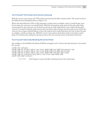
Launch a 100-packet ping from CE1 to CE2:
user@PE1> ping 10.2.2.2 routing-instance CE1 rapid count 100
PING 10.2.2.2 (10.2.2.2): 56 data bytes
!!!!!!!!!!!!!!!!!!!!!!!!!!!!!!!!!!!!!!!!!!!!!!!!!!!!!!!!!!!!!!!!!!!!!!!!!!!!!!!!!!!!!!!!!!!!!!!!!
!!!
--- 10.2.2.2 ping statistics --100 packets transmitted, 100 packets received, 0% packet loss
round-trip min/avg/max/stddev = 0.463/0.809/21.974/2.408 ms](https://image.slidesharecdn.com/packetwalkthrough-131115184203-phpapp02/85/Packet-walkthrough-51-320.jpg)


![52
This Week: A Packet Walkthrough on the M, MX, and T Series
Figure 2.8
Forwarding Path of a Multihop CE-to-CE Ping with Record-route Option
Traceroute from CE to CE (Multihop IPv4/MPLS)
With [protocols mpls icmp-tunneling] configured at P, execute the following
command at PE1 several times:
user@PE1> traceroute 10.2.2.2 routing-instance CE1 no-resolve
traceroute to 10.2.2.2 (10.2.2.2), 30 hops max, 40 byte packets
1 10.1.1.1 0.520 ms 0.303 ms 0.295 ms
2 10.100.1.2 5.624 ms 0.552 ms 0.537 ms
MPLS Label=299904 CoS=0 TTL=1 S=0
MPLS Label=16 CoS=0 TTL=1 S=1
3 10.2.2.1 0.450 ms 0.357 ms 0.352 ms
4 10.2.2.2 0.524 ms 0.455 ms 0.454 ms
user@PE1> traceroute 10.2.2.2 routing-instance CE1 no-resolve
traceroute to 10.2.2.2 (10.2.2.2), 30 hops max, 40 byte packets
1 10.1.1.1 0.455 ms 0.306 ms 0.291 ms
2 10.100.2.2 0.633 ms 4.121 ms 0.536 ms
MPLS Label=299904 CoS=0 TTL=1 S=0
MPLS Label=16 CoS=0 TTL=1 S=1
3 10.2.2.1 0.406 ms 0.366 ms 0.361 ms
4 10.2.2.2 0.529 ms 0.454 ms 0.475 ms
You can see that the good thing about traceroute is that it tells you the path upfront,
but the logic behind it is a bit more complex than it might seem at first.
For example, you can see that the hop displayed at the first line is always the same,
which is natural since there is only one connection CE1-PE1. On the other hand, the
second line is changing from one packet to another. Let’s see why.
As you know, each line of the traceroute output corresponds to an initial TTL value
that starts from 1 and grows by 1 at each line. Figure 2.9 shows the forwarding path
of the various packets sent from CE1, depending on the initial TTL value. You can see
that the second and third hops are actually determined by the Forwarding Plane of
PE1, and P, respectively.](https://image.slidesharecdn.com/packetwalkthrough-131115184203-phpapp02/85/Packet-walkthrough-54-320.jpg)


![Chapter 2: Tracking and Influencing the Path of a Packet
59
Try It Yourself: The Magic Behind record-route Option
With the record-route option, the ICMP packets go up the Control Plane at each hop. But why does this
happen for packets with a remote destination IP? As you can check in the capture, the packets have the
Record Route Option (#7) in the IP header, which means precisely that: Go up the Control Plane. This
option has an IP address list field that gets filled in by transit routers, as you can see in Capture 2.1:
<timestamp> IP (tos 0x0, ttl 64, id 8878, offset 0, flags [none], proto ICMP (1), length 124,
options (RR 0.0.0.0 0.0.0.0 0.0.0.0 0.0.0.0 0.0.0.0 0.0.0.0 0.0.0.0 0.0.0.0 0.0.0.0,EOL))
10.111.1.1 > 10.111.2.2: ICMP echo request, id 4019, seq 0, length 64
<timestamp> IP (tos 0x0, ttl 63, id 8878, offset 0, flags [none], proto ICMP (1), length 124,
options (RR 10.111.11.11, 0.0.0.0 0.0.0.0 0.0.0.0 0.0.0.0 0.0.0.0 0.0.0.0 0.0.0.0 0.0.0.0,EOL))
10.111.1.1 > 10.111.2.2: ICMP echo request, id 4019, seq 0, length 64
<timestamp> IP (tos 0x0, ttl 64, id 56377, offset 0, flags [none], proto ICMP (1), length 124,
options (RR 10.111.11.11, 10.111.2.2, 0.0.0.0 0.0.0.0 0.0.0.0 0.0.0.0 0.0.0.0 0.0.0.0
0.0.0.0,EOL))
10.111.2.2 > 10.111.1.1: ICMP echo reply, id 4019, seq 0, length 64
<timestamp> IP (tos 0x0, ttl 63, id 56377, offset 0, flags [none], proto ICMP (1), length 124,
options (RR 10.111.11.11, 10.111.2.2, 10.111.11.11, 0.0.0.0 0.0.0.0 0.0.0.0 0.0.0.0 0.0.0.0
0.0.0.0,EOL))
10.111.2.2 > 10.111.1.1: ICMP echo reply, id 4019, seq 0, length 64
NOTE The RR option has a limited size, or number of hops that it can record.
Try It Yourself: CE-to-CE Ping Tracking at P-router
The answer is very simple, which doesn’t mean it’s easy! As you saw in Chapter 1, the ICMPv4 packets are
encapsulated in MPLS when they reach P, so you need a MPLS filter:
user@P>
user@P#
user@P#
user@P#
user@P#
user@P#
user@P#
user@P#
user@P#
user@P#
user@P#
user@P#
user@P#
user@P#
configure
edit firewall family mpls filter COUNT-MPLS
set interface-specific
set term DEFAULT then count mpls-packets
top
set interfaces ge-2/3/0 unit 111 family mpls
set interfaces ge-2/3/0 unit 111 family mpls
set interfaces ge-2/3/0 unit 113 family mpls
set interfaces ge-2/3/0 unit 113 family mpls
set interfaces xe-2/0/0 unit 112 family mpls
set interfaces xe-2/0/0 unit 112 family mpls
set interfaces xe-2/0/0 unit 114 family mpls
set interfaces xe-2/0/0 unit 114 family mpls
commit and-quit
CAUTION
filter
filter
filter
filter
filter
filter
filter
filter
input COUNT-MPLS
output COUNT-MPLS
input COUNT-MPLS
output COUNT-MPLS
input COUNT-MPLS
output COUNT-MPLS
input COUNT-MPLS
output COUNT-MPLS
This method is not quite as useful in production routers with end-user MPLS transit
traffic, as that traffic would be counted, too. So one other option would be to use a
different EXP value for ping and match it with the filter, but even that gets complex.
Be cautious here.
Try It Yourself: Capturing MPLS-tagged Traffic with tcpdump
In order to see MPLS control traffic sent from PE2 to the core:
user@PE2> monitor traffic interface ge-1/0/0.113 no-resolve size 2000 matching mpls
user@PE2> monitor traffic interface ge-1/0/1.114 no-resolve size 2000 matching mpls
In order to see MPLS control traffic received by PE2 from the core, there are two options. If you use a
vt- interface at the VRF, then you can capture directly there. But if you use vrf-table-label instead, you
need to find the Label Switched Interface (lsi) unit associated to the VRF first:](https://image.slidesharecdn.com/packetwalkthrough-131115184203-phpapp02/85/Packet-walkthrough-61-320.jpg)


![64
This Week: A Packet Walkthrough on the M, MX, and T Series
Speed
Link is
Speed
Link is
Speed
is 1000Mb
good on GE port 12 connected to device: Other RE
is 1000Mb
good on GE port 13 connected to device: RE-GigE
is 1000Mb
user@P-re0> show chassis ethernet-switch statistics ?
Possible completions:
<[Enter]>
Execute this command
<port>
Port number (0..27)
|
Pipe through a command
In this example, the internal switch sees the REs simply as hosts connected to its
ports 12 and 13. Let’s run a quick connectivity test between two Control Plane
functional components. How about a simple ping from the master RE to the
microkernel of a Line Card? This is possible starting with Junos OS 10.4. You first
need to know the target IP address:
user@P-re0> show arp vpn __juniper_private1__ no-resolve
MAC Address
Address
Interface
Flags
02:00:00:00:00:04 10.0.0.4
em1.0
none
02:00:00:00:00:04 128.0.0.4
em1.0
none
02:00:01:00:00:04 128.0.0.6
em0.0
none
02:00:00:00:00:04 128.0.0.6
em1.0
none
02:00:00:00:00:10 128.0.0.16
em0.0
none
02:00:00:00:00:11 128.0.0.17
em0.0
none
02:00:00:00:00:12 128.0.0.18
em0.0
none
Total entries: 7
The __juniper_private1__ is a private routing instance that the device uses only for
internal communication between the different boards. Since it’s not meant to be
configured, it’s often hidden and it only shows up when it’s explicitly invoked.
TRY THIS Execute: show
route forwarding-table table __juniper_private1__ all and show
route table __juniper_private1__ . Try to remove some of the options and you’ll
likely stop seeing the 128/2 routes, which are not displayed by default.
Out of all the addresses above, which one corresponds to the Line Card in slot #2?
You’ll need to use one more command, like this:
user@P-re0> file show /etc/hosts.junos | match " fpc2$"
128.0.0.18
fpc2
So fpc2 has MAC address 02:00:00:00:00:12, and that corresponds to IPv4 address
128.0.0.18, according to the ARP table. You are now ready to go:
user@P-re0> ping 128.0.0.18 routing-instance __juniper_private1__ count 100 rapid
PING 128.0.0.18 (128.0.0.18): 56 data bytes
!!!!!!!!!!!!!!!!!!!!!!!!!!!!!!!!!!!!!!!!!!!!!!!!!!!!!!!!!!!!!!!!!!!!!!!!!!!!!!!!!!!!!!!!!!!!!!!!
!!!!
--- 128.0.0.18 ping statistics --100 packets transmitted, 100 packets received, 0% packet loss
round-trip min/avg/max/stddev = 0.136/0.151/0.281/0.025 ms
MORE?
Raise the count and spot with show chassis ethernet-switch statistics the ports
of the internal ethernet switch that are used by the flow. Don’t forget that these ports
are also used for all the internal control communication and keep increasing in
steady mode.](https://image.slidesharecdn.com/packetwalkthrough-131115184203-phpapp02/85/Packet-walkthrough-66-320.jpg)
![Chapter 3: Spying on the Private Life of a Packet
TIP
65
In order to thoroughly test any internal or external forwarding path, you can choose
the same bit patterns that are generally used by manufacturing teams while stressing
components. See the last Try It Yourself exercise in Chapter 4 for details.
You can try the same ping from the backup RE and it should work from there, too. If
RE0 is master (check it with show chassis routing-engine), go to RE1:
user@P-re0> request routing-engine login other-routing-engine
user@P-re1> ping 128.0.0.18 routing-instance __juniper_private1__ count 100 rapid
PING 128.0.0.18 (128.0.0.18): 56 data bytes
!!!!!!!!!!!!!!!!!!!!!!!!!!!!!!!!!!!!!!!!!!!!!!!!!!!!!!!!!!!!!!!!!!!!!!!!!!!!!!!!!!!!!!!!!!!!!!!!!
!!!
--- 128.0.0.18 ping statistics --100 packets transmitted, 100 packets received, 0% packet loss
round-trip min/avg/max/stddev = 0.119/0.142/0.270/0.026 ms
user@P-re1> exit
user@P-re0>
What do em0 and em1 stand for? Both are network interfaces at the Routing Engine.
They connect to the same-plane and to the other-plane internal ethernet switches,
respectively. In some sense, you can call them primary and secondary interfaces as in
Table 3.2. They are flagged as P and S in Figure 3.2.
Table 3.2
Names of Ethernet Interfaces at the Routing Engine
MX-Series
M-Series
Model
Primary Interface
@ RE
Secondary Interface
@ RE
Backup RE sends Packets to
Line Cards via ... Interface
MX-5/10/40/80
em0 (1GE)
-
-
MX-240/480/960
em0 (1GE)
em1 (1GE)
Secondary (em1)
M7i
Series
fxp1 (FE)
-
-
M10i
fxp1 (FE)
-
-
M120
em0 (1GE)
em1 (*) (1GE)
Primary (em0)
bcm0 (1GE)
em0 / em1 (**) (FE)
Secondary (em0/em1)
ixgbe0 (1GE)
ixgbe1 (1GE)
Secondary (ixgbe1)
M320
T640/T1600/T4000
T-Series
TX SCC
TXP SFC
(*) Line Cards are not accessible through that interface, only other RE
(**) Depending on the RE model
At terminal #1, connected to P, start a packet capture at the RE primary interface:
user@P-re0> monitor traffic interface em0 no-resolve size 2000 matching icmp
verbose output suppressed, use <detail> or <extensive> for full protocol decode
Address resolution is OFF.
Listening on em0, capture size 2000 bytes
At terminal #2, also connected to P, run an internal ping to fpc2:
user@P-re0> ping 128.0.0.18 routing-instance __juniper_private1__
The capture should show the ICMPv4 exchange:
<timestamp> Out IP 128.0.0.1 > 128.0.0.18: ICMP echo request, id 23088, seq 0, length 64
<timestamp> In IP 128.0.0.18 > 128.0.0.1: ICMP echo reply, id 23088, seq 0, length 64
[...]](https://image.slidesharecdn.com/packetwalkthrough-131115184203-phpapp02/85/Packet-walkthrough-67-320.jpg)


![Table 3.4
Series
Chapter 3: Spying on the Private Life of a Packet
Fabric Plane Distribution per Platform
Model
Fabric Location
Number of Fabric Planes
MX-5/10/40/80
MX-Series
-
-
MX-240
4 per SCB (up to 2 active SCB = 8 active planes)
MX-480
Switch Control Board (SCB)
MX-960
-
M120
T640/T1600/T4000
TX SCC / TXP SFC
-
Control Board (CB)
M10i
M320
T-Series
4 per SCB (up to 2 active SCBs = 8 active planes)
2 per SCB (up to 3 active SCBs = 6 active planes)
M7i
M-Series
69
2 per CB (up to 2 active CBs = 4 active planes)
Switch Interface Board (SIB)
1 per SIB (up to 4 active SIBs = 4 active planes)
Switch Interface Board (SIB)
Three-stage CLOS fabric with 4 active planes
And let’s look at the layout of a MX480 with redundant Switch Control Boards:
user@P-re0> show chassis
Plane State
Uptime
0
Online 1 day, 19
1
Online 1 day, 19
2
Online 1 day, 19
3
Online 1 day, 19
4
Online 1 day, 19
5
Online 1 day, 19
6
Online 1 day, 19
7
Online 1 day, 19
fabric summary
hours,
hours,
hours,
hours,
hours,
hours,
hours,
hours,
50
50
50
50
50
50
50
50
minutes,
minutes,
minutes,
minutes,
minutes,
minutes,
minutes,
minutes,
3
3
3
2
2
2
2
2
seconds
seconds
seconds
seconds
seconds
seconds
seconds
seconds
user@P-re0> show chassis fabric plane-location
------------Fabric Plane Locations------------Plane 0
Control Board 0
Plane 1
Control Board 0
Plane 2
Control Board 0
Plane 3
Control Board 0
Plane 4
Control Board 1
Plane 5
Control Board 1
Plane 6
Control Board 1
Plane 7
Control Board 1
Before moving deeper into the Forwarding Plane, let’s talk briefly about PICs (Physical Interface Cards) and MICs (Modular Interface Cards). From an architectural
point of view, a PIC is a physical card containing a set of functional components
called ports or interfaces. Stated simply, PICs provide connectivity between PFEs and
the outside world. Depending on the Line Card model, PICs can be either independent physical cards, or physically bound to Line Cards, or bundled in a MIC. The
show commands typically take pic as an argument, but the commonly used request
chassis pic [offline|online] operation only works if the PIC is an independent
physical card. Otherwise you need to act on the card it is bound to (fpc or mic).
Execute at P:
user@P-re0> show chassis fpc pic-status
Slot 0 Online
DPCE 40x 1GE R
PIC 0 Online
10x 1GE(LAN)
PIC 1 Online
10x 1GE(LAN)](https://image.slidesharecdn.com/packetwalkthrough-131115184203-phpapp02/85/Packet-walkthrough-71-320.jpg)


![72
This Week: A Packet Walkthrough on the M, MX, and T Series
However, in this example, the numbers on the left of the equal sign are slightly larger
(by around 40 packets) than the numbers on the right: 775 > 735, and 504 > 463.
Try It Yourself: Interpreting PFE Statistics
Why aren’t the formulas exact? The answer is very simple, but not that easy to figure out! Think about it,
figure it out on your own, or cheat and go to the end of the chapter to find out.
In the current situation, it’s natural to expect there to be no traffic flowing through
the fabric at all. However, in this case there is some traffic. Let’s look:
user@P-re0> show class-of-service fabric statistics source 2 destination 2 | match "stat|pps"
Total statistics: High priority
Low priority
Pps
:
39
0
Tx statistics:
High priority
Low priority
Pps
:
39
0
Drop statistics:
High priority
Low priority
Pps
:
0
0
The reason there is some traffic is because the software release used during this
writing – Junos OS 11.4R4.4 – supports a nice feature on MX-Series called fabric
self-ping. Here, each PFE periodically pings itself using its fabric loopback stream:
the path that takes cells from the PFE to the switch fabric, and back to the same PFE.
And it does so for every fabric plane. The goal is to detect PFE-to-fabric connectivity
issues in an independent way. Before the new feature was implemented, end-user
transit traffic was necessary to start detecting fabric failures.
Figure 3.7 illustrates the implementation details of this feature. In pre-Trio PFEs, the
self-ping packets are generated by the microkernel and sent at a low rate using the
PFE-to-fabric queue #7, which has low priority by default but can and should be
changed (with set class-of-service forwarding-classes <name> queue-num 7
priority high, for example). On the other hand, Trio PFEs generate the packets
themselves at a high rate, using a high priority PFE-to-fabric queue. In other words,
self-ping is software-based for pre-Trio, and hardware-based for Trio.
Figure 3.7
PFE Self-ping Through Fabric Forwarding Path
NOTE
MORE?
At the time of this writing T-Series also supports fabric self-ping.
PFE liveness is yet another related feature that periodically sends traffic to other
PFEs through the fabric. This allows for fast internal forwarding path restoration
when a Line Card fails or is abruptly pulled from the chassis. This feature can be
enabled in Junos OS 12.1 or higher in all-Trio MX Series with the [set chassis
network-services enhanced-ip] knob.](https://image.slidesharecdn.com/packetwalkthrough-131115184203-phpapp02/85/Packet-walkthrough-74-320.jpg)


![86
This Week: A Packet Walkthrough on the M, MX, and T Series
You’ve already read about what ping is and where it goes; this chapter deals more
with how it goes: reliably or intermittently? Fast or slow? Big or small? As a whole or
in pieces? The ping options covered in this chapter are widely known and used, but
frequent assumptions are made about them that are not always true. For example:
„„ Myth #1: Intermittent one-hop ping packet loss is an indication of either
hardware issues at the endpoints or physical problems in the link.
„„ Myth #2: If ping shows high latency and jitter, then we have an explanation to
end-user slow network complaints.
Let’s confront these and other myths in this chapter!
Measuring Link Latency
Many network operators use ping to measure the latency of a WAN link. Let’s see
how reliable this is. Execute at PE1:
user@PE1> ping 10.100.1.2 source 10.100.1.1
PING 10.100.1.2 (10.100.1.2): 56 data bytes
64 bytes from 10.100.1.2: icmp_seq=0 ttl=64
64 bytes from 10.100.1.2: icmp_seq=1 ttl=64
64 bytes from 10.100.1.2: icmp_seq=2 ttl=64
[...]
interval 0.1 count 100
time=0.704 ms
time=0.553 ms
time=31.200 ms
--- 10.100.1.2 ping statistics --100 packets transmitted, 100 packets received, 0% packet loss
round-trip min/avg/max/stddev = 0.513/3.150/54.792/7.904 ms
TIP
For latency tests, always make sure you use the source or interface options, just in
case you have default-address-selection configured.
The time values displayed are for the Round Trip Time (RTT) between the time the
echo request is sent, and the echo reply is received. So, assuming symmetrical routing,
which isn’t always the case, the unidirectional latency is typically half of the time.
As you can see, there is a high level of jitter. These latency variations are actually
introduced by the Control Plane components of the sender and receiver, especially by
the Routing Engines, which run non-real-time FreeBSD kernels. Due to the forwarding architecture in Junos OS devices, this extra delay introduced by the Control Plane
does not affect end-user transit traffic at all, so you don’t need to worry that much
about ping jitter.
The average latency can even go higher up if there is a lot of control or exception
traffic queued in the PFE-to-host path. Typical scenarios where this can happen are
aggressive RE-based traffic sampling, or firewall filter log/syslog/reject actions. The
ICMP echo requests/reply compete with this other exception traffic and may be
impacted with higher latency or even discards.
TIP
Look for input/output drops in show pfe statistics traffic, which indicate the
health of the communication channel between Control and Forwarding planes.
So is ping useless for link latency measurements? Not at all. In big international
networks with high latency links, it is a great tool to use. Just take the minimum value
rather than the average/maximum and you’ll have a rough idea of the real link
latency.](https://image.slidesharecdn.com/packetwalkthrough-131115184203-phpapp02/85/Packet-walkthrough-88-320.jpg)


![Chapter 4: Classical Network Applications of Ping
Figure 4.7
99
Fragmentation of ICMPv6 Echo Request at the Source
If, in another terminal connected to PE1, you launch tcpdump to capture the ping
flow, you should see something like this:
user@PE2> monitor traffic interface ge-1/0/1.114 size 2000 no-resolve matching inet6
[...]
<timestamp> In IP6 fc00::100:1:1 > fc00::100:4:1: frag (0|1448) ICMP6, echo request, seq 0, length
1448
<timestamp> In IP6 fc00::100:1:1 > fc00::100:4:1: frag (1448|22)
<timestamp> Out IP6 fc00::100:4:1 > fc00::100:1:1: frag (0|1448) ICMP6, echo reply, seq 0, length
1448
<timestamp> Out IP6 fc00::100:4:1 > fc00::100:1:1: frag (1448|22)
NOTE
If you use the matching
show up.
icmp6 keyword instead, only the first fragments (0|1448)
Note that there is no DF flag in IPv6. Even if the do-not-fragment option exists, it
makes no change in the IPv6 packet so there is no point in using it.
Table 4.1
New ICMP Types and Codes (seen in this chapter)
ICMPv4 (IP Protocol 1)
ICMPv6 (IPv6 Next Header 58)
Type
Code
Description
Type
Code
Description
3
4
Destination Unreachable, Fragmentation Needed
2
0
Too Big](https://image.slidesharecdn.com/packetwalkthrough-131115184203-phpapp02/85/Packet-walkthrough-101-320.jpg)


![Chapter 5: One Loop to Rule Them All
107
Half-Duplex Loops
Looping interfaces is a traditional troubleshooting method to verify the integrity of
a link. Figure 5.1 shows three half-duplex loopback flavors, from top to bottom:
„„ Local software loopback: the physical interface is configured as loopback
[local] at R1. The outgoing packets reach the PIC and are returned back to
the PFE, where they are looked up and forwarded again. This chapter focuses
on this mode.
„„ Physical half-duplex loopback: With the help of optical equipment, the two
strands of a fiber are connected to each other. No configuration is required on
the routers. The loop can be completed next to R1, next to R2, or anywhere
else along the transmission path.
„„ Remote software loopback: physical interface in remote loopback mode at R2
(or at a transmission device in the path). The incoming signal at R2 reaches the
PIC and is returned back to the fiber/cable. One copy of the packets is sent to
the PFE at R2, so packets can be counted there as well (interface statistics and
firewall filter counters).
Figure 5.1
Half-duplex Port Loopback Techniques
Due to their great flexibility and low requirements, this book uses local software
half-duplex loops as the preferred option for general applications beyond link
troubleshooting. It’s true, they are not suitable for Control Plane tests involving
different Logical Systems or Virtual Routers running routing protocols with each
other, but in the context of pure Forwarding Plane tests, they simply rock!
In order to generate traffic, there are two classic networking options. If you ping an
IPv4/IPv6 address locally configured at the router’s interface, make sure you use the
interface and bypass-routing options, otherwise the packet won’t leave the
Control Plane. If you ping the remote address of the link, the packet will loop until
TTL expires. (Both options are covered in detail later in this chapter.)](https://image.slidesharecdn.com/packetwalkthrough-131115184203-phpapp02/85/Packet-walkthrough-109-320.jpg)


![120
This Week: A Packet Walkthrough on the M, MX, and T Series
user@P> configure
user@P# edit protocols mpls
user@P# set static-label-switched-path
10.202.1.2
user@P# set static-label-switched-path
user@P# set static-label-switched-path
user@P# set static-label-switched-path
user@P# top
user@P# commit and-quit
SNAKE-A-1 ingress to 10.202.100.1 push 1000001 next-hop
SNAKE-A-2 transit 1000001 swap 1000002 next-hop 10.202.2.2
SNAKE-A-3 transit 1000002 swap 1000003 next-hop 10.202.1.2
SNAKE-A-4 transit 1000003 pop next-hop 10.202.2.2
user@P> show route 10.202.100.1 exact
inet.3: 5 destinations, 5 routes (5 active, 0 holddown, 0 hidden)
+ = Active Route, - = Last Active, * = Both
10.202.100.1/32
*[MPLS/6/1] 00:00:14, metric 0
> to 10.202.1.2 via ge-2/3/1.202, Push 1000001
You need a route in inet.0 to target your ping. There are several ways to achieve that,
let’s choose probably the simplest one:
user@P> configure
user@P# set routing-options static route 10.202.100.100 next-hop 10.202.100.1 resolve
user@P# commit and-quit
user@P> show route 10.202.100.100 exact
inet.0: 45 destinations, 56 routes (45 active, 0 holddown, 0 hidden)
+ = Active Route, - = Last Active, * = Both
10.202.100.100/32 *[Static/5] 00:00:06, metric2 0
> to 10.202.1.2 via ge-2/3/1.202, Push 1000001
Now you can now follow the snake through all its coils:
user@P> show route forwarding-table destination 10.202.100.100 table default
Routing table: default.inet
Internet:
Destination
Type RtRef Next hop
Type Index NhRef Netif
10.202.100.100/32 user
0
indr 1048582
2
10.202.1.2
Push 1000001 810
2 ge-2/3/1.202
user@P> show route forwarding-table label 1000001 table default
Routing table: default.mpls
MPLS:
Destination
Type RtRef Next hop
Type Index NhRef Netif
1000001
user
0 10.202.2.2
Swap 1000002 753
2 xe-2/0/1.202
user@P> show route forwarding-table label 1000002 table default
Routing table: default.mpls
MPLS:
Destination
Type RtRef Next hop
Type Index NhRef Netif
1000002
user
0 10.202.1.2
Swap 1000003 809
2 ge-2/3/1.202
user@P> show route forwarding-table label 1000003 table default
Routing table: default.mpls
MPLS:
Destination
Type RtRef Next hop
Type Index NhRef Netif
1000003
user
0 10.202.2.2
Pop
812
2 xe-2/0/1.202
1000003(S=0)
user
0 10.202.2.2
Pop
813
2 xe-2/0/1.202](https://image.slidesharecdn.com/packetwalkthrough-131115184203-phpapp02/85/Packet-walkthrough-122-320.jpg)


![124
This Week: A Packet Walkthrough on the M, MX, and T Series
The number of packets matches the default
usual.
ttl value (64). So far, it’s business as
Actually, no traffic is being mirrored yet. You could copy traffic from any other
source interface to the mirror destination xe-2/1/0.0, but this just duplicates the
packets. If you want to fill a 10GE interface with just one ping, you need to do
something crazier. How about making xe-2/1/0.0 not only the mirror destination,
but also the mirror source?
In that case, if a packet is sent out of xe-2/1/0.0, when it’s received back from the
loop, the Trio PFE performs two actions:
„„ It processes the packet normally. If TTL>1, then the PFE decreases TTL and sets
the packet next hop to xe-2/1/0.0 mac 00:23:9c:9a:d2:e6. If TTL=1, then the
PFE flags it as an exception packet and sets the host (Line Card microkernel) as
next hop.
„„ It sends the packet to the fabric loopback stream (see the explanation after
Table 3.5). Once the packet is back from the fabric, the PFE sends a copy to the
mirror destination, which is precisely xe-2/1/0.0 itself.
NOTE
This technique also works in pre-Trio platforms, but the internal implementation is
different.
The outcome is one packet whose copies fill up the port:
user@P>
user@P#
user@P#
user@P#
configure
set firewall family inet filter MIRROR-INET term MIRROR then port-mirror
set interfaces xe-2/1/0 unit 0 family inet filter input MIRROR-INET
commit and-quit
user@P> ping 10.200.1.2 count 1 no-resolve wait 1 ttl 10
PING 10.200.1.2 (10.200.1.2): 56 data bytes
/* Lots of Time to live exceeded messages */
--- 10.200.1.2 ping statistics --1 packets transmitted, 0 packets received, 100% packet loss
user@P> show interfaces xe-2/1/0 | match pps
Input rate
: 6885362872 bps (10246075 pps)
Output rate
: 6885361520 bps (10246073 pps)
user@P> show interfaces queue xe-2/1/0 egress | except " 0 "
Physical interface: xe-2/1/0, Enabled, Physical link is Up
Interface index: 216, SNMP ifIndex: 607
Forwarding classes: 16 supported, 4 in use
Egress queues: 8 supported, 4 in use
Queue: 0, Forwarding classes: best-effort
Queued:
Packets
:
278889305
10245653 pps
Bytes
:
34024495210
9999757968 bps
Transmitted:
Packets
:
227255947
10245653 pps
Bytes
:
27725225534
9999757968 bps
[...]
NOTE The show
interfaces queue command is taking into account Layer 2 headers.
Why are there precisely 10Gbps and no drops? How can it be that precise? And if you
sent one more TTL=10 packet, there would probably still be no drops. It’s because](https://image.slidesharecdn.com/packetwalkthrough-131115184203-phpapp02/85/Packet-walkthrough-126-320.jpg)


![128
This Week: A Packet Walkthrough on the M, MX, and T Series
TIP
You can load the configuration with load
set terminal or load set <filename>.
Once the configuration is applied, execute at P:
user@P> show route 10.203.100.1
inet.3: 4 destinations, 4 routes (4 active, 0 holddown, 0 hidden)
+ = Active Route, - = Last Active, * = Both
10.203.100.1/32
*[MPLS/6/1] 00:00:02, metric 0
> to 10.203.1.2 via lt-2/0/0.1, Push 1001001
You need a route in inet.0 to use it as the ping target:
user@P> configure
user@P# set routing-options static route 10.203.100.100/32 next-hop 10.203.100.1 resolve
user@P# commit and-quit
user@P> show route 10.203.100.100
inet.0: 22 destinations, 23 routes (22 active, 0 holddown, 0 hidden)
+ = Active Route, - = Last Active, * = Both
10.203.100.100/32 *[Static/5] 00:00:27, metric2 0
> to 10.203.1.2 via lt-2/0/0.1, Push 1001001
TRY THIS
Follow the snake hop by hop at the forwarding table level.
Everything is ready for the first 10,000-times-replicating packet:
user@P> clear interfaces statistics all
user@P> ping 10.203.100.100 count 1 ttl 100 no-resolve wait 1
PING 10.203.100.100 (10.203.100.100): 56 data bytes
36 bytes from 10.203.1.1: Time to live exceeded
Vr HL TOS Len ID Flg off TTL Pro cks
Src
Dst
4 5 00 0054 c0be 0 0000 01 01 7df0 10.203.1.1 10.203.100.100
--- 10.203.100.100 ping statistics --1 packets transmitted, 0 packets received, 100% packet loss
user@P> show interfaces lt-2/0/0.1 statistics | match packets
Input packets : 5000
Output packets: 5000
This is the same ICMPv4 echo request going 5,000 times forth and 5,000 times back.
How about mirroring all the copies out of P?
user@P>
user@P#
user@P#
user@P#
configure
set firewall family ccc filter MIRROR-CCC term MIRROR then port-mirror
set interfaces lt-2/0/0 unit 11 family ccc filter input MIRROR-CCC
set interfaces lt-2/1/0 unit 11 family ccc filter input MIRROR-CCC
user@P# set interfaces ge-2/3/0 encapsulation flexible-ethernet-services
user@P# set interfaces ge-2/3/0 unit 203 vlan-id 203 encapsulation vlan-bridge family bridge
user@P# set bridge-domains MIRROR interface ge-2/3/0.203
user@P# set forwarding-options port-mirroring input rate 1
user@P# set forwarding-options port-mirroring family ccc output interface ge-2/3/0.203
user@P# commit and-quit](https://image.slidesharecdn.com/packetwalkthrough-131115184203-phpapp02/85/Packet-walkthrough-130-320.jpg)


![Chapter 5: One Loop to Rule Them All
131
You can configure the next hop group using this Perl script:
#!/usr/bin/perl
(my $interface, my $mac) = @ARGV;
if ((!$ARGV[0]) || (!$ARGV[1])) {
print "Usage: perl next-hop-group.pl <physical-interface> <mac-address>n";
exit;
}
for (my $i=1; $i<41; $i++) {
print "set forwarding-options next-hop-group MULTIPLY interface
".$interface.".".($i+150)." next-hop 10.202.".($i+150).".2n";
print "set interfaces ".$interface." unit ".($i+150)." vlan-id ".($i+150)." family inet
address 10.202.".($i+150).".1/30 arp 10.202.".($i+150).".2 mac ".$mac."n";
}
One simple value for the MAC address option is a Juniper generic one:
$ perl next-hop-group.pl ge-2/3/0 00:23:9c:00:00:00
/* Output Suppressed */
Once the next-hop group is configured, you just need to mirror the input traffic at
ge-2/3/1.202:
user@P>
user@P#
user@P#
user@P#
user@P#
user@P#
configure
delete forwarding-options port-mirroring family inet
set forwarding-options port-mirroring family inet output next-hop-group MULTIPLY
set firewall family inet filter MIRROR-INET term MIRROR then port-mirror
set interfaces ge-2/3/1.202 family inet filter input MIRROR-INET
commit and-quit
Leave running:
user@P> ping 10.202.1.2 interval 0.1 ttl 250 no-resolve size 1460
/* Output suppressed */
In another terminal, check that the egress port is saturated, and as expected:
user@P> show interfaces queue ge-2/3/0 | except " 0"
Physical interface: ge-2/3/0, Enabled, Physical link is Up
Interface index: 228, SNMP ifIndex: 16036
Forwarding classes: 16 supported, 4 in use
Egress queues: 8 supported, 4 in use
Queue: 0, Forwarding classes: best-effort
Queued:
Packets
:
1800006
98550 pps
Bytes
:
2754000546
1206261240 bps
Transmitted:
Packets
:
1477254
80989 pps
Bytes
:
2260189986
991305560 bps
Tail-dropped packets :
322752
17561 pps
Queue: 1, Forwarding classes: expedited-forwarding
Queued:
Queue: 2, Forwarding classes: assured-forwarding
Queued:
Queue: 3, Forwarding classes: network-control
Queued:
Bytes
:
1656
512 bps
Bytes
:
1656
512 bps](https://image.slidesharecdn.com/packetwalkthrough-131115184203-phpapp02/85/Packet-walkthrough-133-320.jpg)


![Chapter 5: One Loop to Rule Them All
137
user@P> configure
user@P# set firewall family inet filter lo0-COS term ICMP then dscp 40
user@P> commit and-quit
user@P> clear firewall all
user@P> clear interfaces statistics all
user@P> ping 10.204.1.2 count 1 no-resolve wait 1 tos 0
/* Output suppressed */
user@P> show firewall | match ge-2/3/1.204 | except " 0" | except filter
prec-5-ge-2/3/1.204-i
5376
64
user@P> configure
user@P# delete firewall family inet filter lo0-COS term ICMP then dscp
user@P# commit and-quit
NOTE
An older knob [edit class-of-service host-outbound-traffic] also allows you
to remap outbound Control Traffic to a different Forwarding Class and DSCP than
the one initially chosen by the RE. This feature is less flexible since it applies to all
the traffic with no granularity.
Going back to Figure 5.14, how can you classify the transit packets as expeditedforwarding? There are several options, of which the most flexible is changing the
firewall filter chain currently applied to ge-2/3/1.204. The results are in Figure 5.15.
Execute at P:
user@P>
user@P#
user@P#
user@P#
user@P#
configure
edit firewall family inet filter PREC-TO-FC term PREC5
set from precedence 5
set then forwarding-class expedited-forwarding
set then next term
/* since this is the last term, it will go to the next filter in the chain */
user@P# set interfaces ge-2/3/1.204 family inet filter input-list [ PREC-TO-FC PRECEDENCE-CHECK ]
user@P# commit and-quit
user@P> clear interfaces statistics all
user@P> clear firewall all
user@P> ping 10.204.1.2 count 1 no-resolve wait 1 tos 160
/* Output suppressed */
user@P> show interfaces queue ge-2/3/1.204 | except " 0 "
Logical interface ge-2/3/1.204 (Index 425) (SNMP ifIndex 15596)
Forwarding classes: 16 supported, 4 in use
Egress queues: 8 supported, 4 in use
Burst size: 0
Queue: 0, Forwarding classes: best-effort
Queued:
Queue: 1, Forwarding classes: expedited-forwarding
Queued:
Packets
:
64
0 pps
Bytes
:
8064
0 bps
Transmitted:
Packets
:
64
0 pps
Bytes
:
8064
0 bps
Queue: 2, Forwarding classes: assured-forwarding
Queued:
Queue: 3, Forwarding classes: network-control
Queued:
user@P> show firewall | match ge-2/3/1.204 | except " 0" | except filter
prec-5-ge-2/3/1.204-i
5376
64](https://image.slidesharecdn.com/packetwalkthrough-131115184203-phpapp02/85/Packet-walkthrough-139-320.jpg)


![144
This Week: A Packet Walkthrough on the M, MX, and T Series
mpls.0: 70 destinations, 70 routes (70 active, 0 holddown, 0 hidden)
+ = Active Route, - = Last Active, * = Both
16
*[VPN/0] 00:00:25
to table VRF-COS.inet.0, Pop
Next, define a static LSP leading to the VRF:
user@P> configure
user@P# edit protocols mpls
user@P# set static-label-switched-path SNAKE-D-1 ingress to 10.205.100.1 push 1003001 next-hop
10.204.1.2
user@P# set static-label-switched-path SNAKE-D-2 transit 1003001 swap 16 next-hop 10.204.1.2
user@P# top
user@P# set routing-options static route 10.205.100.100 next-hop 10.205.100.1 resolve
Let’s follow the snake up to its destination:
user@P> show route forwarding-table destination 10.205.100.100 table default
Routing table: default.inet
Internet:
Destination
Type RtRef Next hop
Type Index NhRef Netif
10.205.100.100/32 user
0
indr 1048576
2
10.204.1.2
Push 1003001 1119
2 ge-2/3/1.204
user@P> show route label 1003001
mpls.0: 71 destinations, 71 routes (71 active, 0 holddown, 0 hidden)
+ = Active Route, - = Last Active, * = Both
1003001
*[MPLS/6] 00:00:59, metric 1
> to 10.204.1.2 via ge-2/3/1.204, Swap 16
user@P> show route label 16
mpls.0: 71 destinations, 71 routes (71 active, 0 holddown, 0 hidden)
+ = Active Route, - = Last Active, * = Both
16
*[VPN/0] 00:21:42
to table VRF-COS.inet.0, Pop
user@P> show route forwarding-table destination 10.205.100.100 table VRF-COS
Routing table: VRF-COS.inet
Internet:
Destination
Type RtRef Next hop
Type Index NhRef Netif
10.205.100.100/32 user
0 10.205.1.2
ucst 1118
3 ge-2/3/1.205
Now, make it work with the usual procedure:
user@P> clear firewall all
user@P> clear interfaces statistics all
user@P> ping 10.205.100.100 count 1 no-resolve wait 1 ttl 3 tos 160
PING 10.205.100.100 (10.205.100.100): 56 data bytes
--- 10.205.100.100 ping statistics --1 packets transmitted, 0 packets received, 100% packet loss
user@P> show interfaces queue ge-2/3/1.205 | except " 0 "
Logical interface ge-2/3/1.205 (Index 378) (SNMP ifIndex 15597)
Forwarding classes: 16 supported, 4 in use
Egress queues: 8 supported, 4 in use
Burst size: 0](https://image.slidesharecdn.com/packetwalkthrough-131115184203-phpapp02/85/Packet-walkthrough-146-320.jpg)


![152
This Week: A Packet Walkthrough on the M, MX, and T Series
Answers to Try It Yourself Sections of Chapter 5
Try It Yourself: Measuring Throughput with Snake Tests
First, in a full duplex test involving 20 ports, the number of hops in one direction is half of the number of
links: 10.
The original question is tough to answer from a mathematical perspective. The reverse is easier, though: if the
probability of a packet to be dropped in a hop is N%, what would be the measured loss in the snake test?
Assume that the physical links are healthy and all the routes are in place. If a packet doesn’t reach the receiver,
there are 10 possibilities: it may have been dropped in hop #1, or in hop #2, etc., or finally in hop #10. You
already know the probability for the packet to be dropped in hop #1: N%. For the packet to be dropped in hop
#2, two things must happen: first, that it wasn’t dropped in hop #1, and second, that once it reaches hop #2 it
is dropped there. The probabilities of these two events are (100-N)% and N%, respectively. The probability
for the combined event is: [(100-N)/100]*N %. You can iterate this logic with the following perl script:
#!/usr/bin/perl
(my $number_of_hops, my $per_hop_drop_percent) = @ARGV;
if (($ARGV[0] < 1) || ($ARGV[1] < 0) || ($ARGV[1] > 100)) {
print "Usage: perl snake-drop-probability.pl <number-of-hops> <per-hop-drop-percent>n";
exit;
}
my $drop_probability = $per_hop_drop_percent / 100;
if ($number_of_hops > 0) {
for ($i = 1; $i < $number_of_hops; $i++) {
$drop_probability += ($per_hop_drop_percent / 100) * (1 - $drop_probability);
}
}
my $drop_percent = 100 * $drop_probability;
print "The total drop probability in the path is ".$drop_percent."%n";
Then do a binary search, trying different possible values of $per_hop_drop_percent until you hit a $drop_percent of 10%. The $number_of_hops is always 10:
$ perl snake-drop-probability.pl 10 10
The total drop probability in the path is 65.13215599%
$ perl snake-drop-probability.pl 10 1
The total drop probability in the path is 9.56179249911955%
$ perl snake-drop-probability.pl 10 1.05
The total drop probability in the path is 10.0175144319432%
$ perl snake-drop-probability.pl 10 1.04
The total drop probability in the path is 9.92653573725331%
So the real throughput is 100-1.05 = 98.95 %. Much better than 90%, wouldn’t you say?
CAUTION
This theory assumes that there is a common bottleneck for all hops. If that’s not the
case, things get more complex. Conclusion: if possible, try not to measure throughput
with snake tests!](https://image.slidesharecdn.com/packetwalkthrough-131115184203-phpapp02/85/Packet-walkthrough-154-320.jpg)


![164
This Week: A Packet Walkthrough on the M, MX, and T Series
term REST {
then accept;
}
}
}
}
routing-instances {
CE2 {
instance-type virtual-router;
interface ge-1/0/0.102;
routing-options {
rib CE2.inet6.0 {
static {
route ::/0 next-hop fc00::2:1;
}
}
}
}
VRF2 {
instance-type vrf;
interface ge-1/0/1.102;
route-distinguisher 65000:1;
vrf-target target:65000:100;
vrf-table-label;
}
}
Initial Configuration of the Switch
X (EX4200)
The switch performs a double role. First, it allows for flexible connections between
routers, and second, it mirrors traffic towards the host.
interfaces {
ge-0/0/10 {
mtu 1600;
unit 0 {
family ethernet-switching {
port-mode access;
vlan {
members v120;
}
}
}
}
ge-0/0/11 {
mtu 1600;
unit 0 {
family ethernet-switching {
port-mode trunk;
vlan {
members [ v101 v111 ];
}
filter {
input NO-ARP;
}
}
}
}](https://image.slidesharecdn.com/packetwalkthrough-131115184203-phpapp02/85/Packet-walkthrough-166-320.jpg)
![ge-0/0/12 {
mtu 1600;
unit 0 {
family ethernet-switching
port-mode trunk;
vlan {
members [ v111 v113
}
}
}
}
ge-0/0/13 {
mtu 1600;
unit 0 {
family ethernet-switching
port-mode trunk;
vlan {
members [ v113 v102
}
}
}
}
ge-0/0/14 {
mtu 1600;
unit 0 {
family ethernet-switching
port-mode trunk;
vlan {
members [ v101 v112
}
filter {
input NO-ARP;
}
}
}
}
ge-0/0/15 {
mtu 1600;
unit 0 {
family ethernet-switching
port-mode trunk;
vlan {
members [ v114 v102
}
}
}
}
xe-0/1/0 {
mtu 1600;
unit 0 {
family ethernet-switching
port-mode trunk;
vlan {
members [ v112 v114
}
}
}
}
}
firewall {
family ethernet-switching {
filter NO-ARP {
term NO-ARP {
Appendix
{
];
{
];
{
];
{
];
{
];
165](https://image.slidesharecdn.com/packetwalkthrough-131115184203-phpapp02/85/Packet-walkthrough-167-320.jpg)

![Appendix
167
Initial Configuration of the Host
H (FreeBSD)
The host just needs an IP address configured at the interface where tcpdump is run.
[root@H ~]# ifconfig bce1 10.100.5.1 netmask 255.255.255.252
[root@H ~]#
Basic Connectivity Tests
PE1, P, and PE2 are connected to each other in Autonomous System 65000, with
IS-IS and LDP running in the core links. Later in Chapter 1, there will be a Multiprotocol IBGP session between PE1 and PE2, initially used to exchange inet-vpn
unicast prefixes of the VRFs.
Check one-hop IP connectivity is fine at the backbone, by executing at P:
user@P>
user@P>
user@P>
user@P>
ping
ping
ping
ping
10.100.1.1
10.100.2.1
10.100.3.1
10.100.4.1
count
count
count
count
1
1
1
1
Check one-hop IP connectivity is broken at the VRF1-CE1 and VRF2-CE2 links:
user@PE1> ping 10.1.1.1 routing-instance CE1 count 1
user@PE2> ping 10.2.2.1 routing-instance CE2 count 1
IMPORTANT
The later two pings are expected to fail at this stage.
Verify that everything is fine at the ISIS and LDP level. The following commands are
executed on PE1, you can do similar checks for P and PE2, too:
user@PE1> show isis adjacency
Interface
System
ge-1/0/0.111
P
ge-1/0/1.112
P
user@PE1> show ldp neighbor
Address
Interface
10.100.1.2
ge-1/0/0.111
10.100.2.2
ge-1/0/1.112
L State
2 Up
2 Up
Hold (secs) SNPA
26
21
Label space ID
10.111.2.2:0
10.111.2.2:0
user@PE1> show ldp session
Address
State
Connection
10.111.2.2
Operational Open
Hold time
11
14
Hold time
28
No BGP sessions are established, since you did not configure any neighbors yet (that
is expected):
user@PE1> show bgp summary
Groups: 0 Peers: 0 Down peers: 0
Table
Tot Paths Act Paths Suppressed
bgp.l3vpn.0
0
0
0
History Damp State
0
0
Pending
0
user@PE1> show route table CE1
CE1.inet.0: 2 destinations, 2 routes (2 active, 0 holddown, 0 hidden)
+ = Active Route, - = Last Active, * = Both](https://image.slidesharecdn.com/packetwalkthrough-131115184203-phpapp02/85/Packet-walkthrough-169-320.jpg)
![168
This Week: A Packet Walkthrough on the M, MX, and T Series
10.1.1.0/30
10.1.1.2/32
*[Direct/0] 02:35:31
> via ge-1/0/0.101
*[Local/0] 02:35:51
Local via ge-1/0/0.101
CE1.inet6.0: 5 destinations, 5 routes (5 active, 0 holddown, 0 hidden)
+ = Active Route, - = Last Active, * = Both
::/0
*[Static/5] 00:08:02
> to fc00::1:1 via ge-1/0/0.101
fc00::1:0/112
*[Direct/0] 00:22:04
> via ge-1/0/0.101
fc00::1:2/128
*[Local/0] 00:22:04
Local via ge-1/0/0.101
fe80::/64
*[Direct/0] 00:22:04
> via ge-1/0/0.101
fe80::5e5e:ab00:650a:c360/128
*[Local/0] 00:22:04
Local via ge-1/0/0.101
user@PE1> show route table VRF1
VRF1.inet.0: 2 destinations, 2 routes (2 active, 0 holddown, 0 hidden)
+ = Active Route, - = Last Active, * = Both
10.1.1.0/30
10.1.1.1/32
*[Direct/0] 01:35:06
> via ge-1/0/1.101
*[Local/0] 01:35:06
Local via ge-1/0/1.101
VRF1.inet6.0: 4 destinations, 4 routes (4 active, 0 holddown, 0 hidden)
+ = Active Route, - = Last Active, * = Both
fc00::1:0/112
*[Direct/0] 00:22:33
> via ge-1/0/1.101
fc00::1:1/128
*[Local/0] 00:22:33
Local via ge-1/0/1.101
fe80::/64
*[Direct/0] 00:22:33
> via ge-1/0/1.101
fe80::5e5e:ab00:650a:c361/128
*[Local/0] 00:22:33
Local via ge-1/0/1.101](https://image.slidesharecdn.com/packetwalkthrough-131115184203-phpapp02/85/Packet-walkthrough-170-320.jpg)

This book provides a detailed overview of using ping and traceroute to troubleshoot Juniper M, MX, and T series routers. It explores how these basic tools can uncover details about the internal architecture and components of the routers. The book shows how ping and traceroute can be used to test features, monitor performance, and isolate network issues. Readers will learn new techniques for tracking the path of packets through the network and inside the router. The goal is to help network operators quickly solve problems by gaining a deeper understanding of how packets flow through Juniper routers using only ping and traceroute.