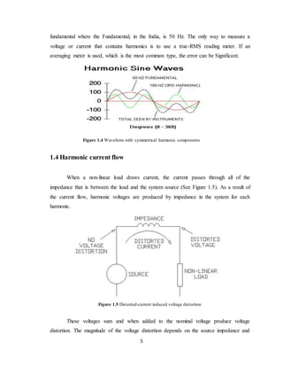
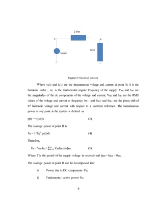
1
CHAPTER-1
Identification and Reduction of Harmonics – An
Overview
1.1 Introduction
The objective of the electric utility is to deliver sinusoidal voltage at fairly
constant magnitude throughout their system. This objective is complicated by the fact
that there are loads on the system that produce harmonic currents. These currents result in
distorted voltages and currents that can adversely impact the system performance in
different ways. As the number of harmonic producing loads has increased over the years,
it has become necessary to address their influence when making any changes to a system.
Evolution of dispersed generation and deregulated electricity markets will force
electric utility to be more concerned about power-quality (PQ) problems, especially
harmonics. There are various sources of harmonic pollution in the power network, with
non-linear loads and dispersed generators that use power-conditioning units as the main
sources.
Identifying the source of harmonic pollution is the first step towards improving
the PQ of the network. This can be achieved either by: (1) distributed synchronous
measurements at the points of the system, or (2) single-point measurements at the point
of common coupling (PCC). Distributed synchronous measurements can provide detailed
information about the harmonic content and harmonic flow. However, this method
requires the installation of numerous sensors in order to monitor nodes of the network.
Moreover, a means of communication is necessary to synchronize the monitored data,
thus increasing the complexity and cost of the system. On the contrary, single point
measurements are simple and cost effective, as they are performed at a specific node in
2
the network to decide whether the load connected at that node is a source of harmonic
pollution.
A number of methods have been proposed to identify the source of harmonics
using single-pint measurements. However, some of these methods are controversial, as
they are based on new concepts that still need thorough investigation before confirming
their complete success.
The total harmonic power (THP) method is simple method that uses the sign of
THP at a specific node to decide on whether the source of harmonic pollution is upstream
or downstream from this node.
1.2 HARMONICS
Power system Harmonics are integer multiples of the fundamental power system
frequency. A normal alternating current in the power system has a sinusoidal wave form.
When a sinusoidal voltage is applied to a linear load, the current drawn is also sinusoidal
at the same frequency (though usually not in phase with the voltage), on the contrary the
non-linear loads draws non sinusoidal or pulsating current. Any non-sinusoidal wave form
can be mathematically resolved in to a series of sinusoidal components. The first
component is called as fundamental and the remaining components whose frequencies
are integral multiples of the fundamental frequency are known as harmonics. If the
fundamental frequency is 50HZ then the 2
nd
harmonics will have a frequency of 100 HZ
and the 3
rd
will have 150 HZ and so on.
The figure depicted below explains the fundamental with third and fifth Harmonics
3
Figure 1.1 Fundamental with third and fifth Harmonics
High levels of harmonics in a power system can create voltage distortion resulting
in power quality problems. The major effect of harmonic distortion includes overheating
of the equipments like motors, transformers, cables, capacitors, power electronics etc.,
leading to their premature failure besides there will be some more ill effects which are
specific to each type of equipments like, nuisance tripping, erratic operation of relays and
control equipments, severe over loading of capacitors, breakdown of electronics
equipments, very high internal current in the 3PH – 4 wire system.
To fully appreciate the impact of this phenomenon, there are two important
concepts to bear in mind with regard to power system harmonics. The first is the nature
of harmonic-current producing loads (non-linear loads) and the second is the way in
which harmonic currents flow and how the resulting harmonic voltages develop.
1.3 Linear and non-linear loads
1.3.1 Linear loads
A linear element in a power system is a component in which the current is
proportional to the voltage. In general, this means that the current wave shape will be the
4
same as the voltage (See Figure 1.2). Typical examples of linear loads include motors,
heaters and incandescent lamps.
Figure 1.2 Voltage and current waveforms for linear
1.3.2 Non-linear loads
On the other hand, the current wave shape on a non-linear load is not the same as
the voltage (See Figure 1.3). Typical examples of non-linear loads include rectifiers
(power supplies, UPS units, discharge lighting), adjustable speed motor drives,
ferromagnetic devices, DC motor drives and arcing equipment.
Figure 1.3 Voltage and current waveforms for non-linear loads
The current drawn by non-linear loads is not sinusoidal but it is periodic, meaning
that the current wave looks the same from cycle to cycle. Periodic waveforms can be
described mathematically as a series of sinusoidal waveforms that have been summed
together (See Figure 1.4). The sinusoidal components are integer multiples of the
5
fundamental where the Fundamental, in the India, is 50 Hz. The only way to measure a
voltage or current that contains harmonics is to use a true-RMS reading meter. If an
averaging meter is used, which is the most common type, the error can be Significant.
Figure 1.4 Waveform with symmetrical harmonic components
1.4 Harmonic current flow
When a non-linear load draws current, the current passes through all of the
impedance that is between the load and the system source (See Figure 1.5). As a result of
the current flow, harmonic voltages are produced by impedance in the system for each
harmonic.
Figure 1.5 Distorted-current induced voltage distortion
These voltages sum and when added to the nominal voltage produce voltage
distortion. The magnitude of the voltage distortion depends on the source impedance and
6
the harmonic voltage produced. If the source impedance is low then the voltage
distortion will be low. If a significant portion of the load becomes non-linear (harmonic
currents increase) and/or when a resonant condition prevails (system impedance
increases), the voltage can increase dramatically.
Power systems are able to absorb a considerable amount of current distortion
without problems and the distortion produced by a facility may be below levels
recommended in IEEE 519. However, the collective effect of many industrial customers,
taken together, may impact a distribution system. When problems arise, they are usually
associated with resonant conditions.
1.5 Effects of Harmonics
The actual problems of any building/industry will vary depending on the type and
number of installed harmonics producing loads. Most electrical network can withstand
nonlinear loads of up to 15% of the total electrical system capacity without concern but
when the nonlinear loads exceed 15% some non-expected negative consequences can be
expected.
The following is a short summary of most problems caused by harmonics:
(i) Blinking of incandescent lights-transformer saturation
(ii) Capacitor failure-harmonics resonance
(iii) Circuit breaker tripping-inductive heating and over loading
(iv) Computer malfunctioning-voltage distortion
(v) Transformer failure-inducting
7
(vi) Motor failure-inductive heating
(vii) Fuses blowing for no apparent reason-inductive heating & over load
(viii) Electronic component shut down- voltage distortion
(ix) Flickering of florescent lights-transformer saturation
The heating effects of harmonic currents can cause destruction of equipment,
conductors, and fires. The results can be unpredictable legal and financial ramifications
apart from safety risks. Voltage distortions can lead to overheating of equipment failure,
expensive down time and maintenance difficulties. The problems associated with
nonlinear loads were once limited to isolated devicesand computer rooms, but now the
problem appear through the entire network and utility system.
The point at which the harmonic limits are applied is called the point of common
coupling (PCC). When the input transformer is the point of measurement then the PCC
refers to this point where the facility electrical system is common to the facility of
additional consumers. If there is a distortion present on the electrical power system at this
point it may be experienced by the neigh boring facilities as well. So we need to avoid
this situation.
1.6 Distribution System
In this project the case studies is performed by the use radial distribution system.
A radial system has only one power source for a group of customers. A power failure,
short-circuit, or a downed power line would interrupt power in the entire line which must
be fixed before power can be restored. The Radial distribution system is the cheapest to
build, and is widely used in sparsely populated areas.
8
Figure 1.6 Radial Distribution System
1.7 TOTAL HARMONIC POWER METHOD
The fundamentals of the THP method can be illustrated by using the circuit
shown in figure. An ideal sinusoidal voltage source is connected to a non-linear load
through the system impedance. The non-linear load generates harmonic currents that flow
in the system causing voltage distortion at point B. This voltage distortion depends on
both the harmonic currents and the system impedance at harmonic frequencies. The
distorted current and voltage at point B can be expressed by Fourier series as
vB(t) = VBo+ ∑ √2V
∞
𝑛=1
Bhsin(hw1t + θBhV) (1)
iB(t) = IBo+ ∑ √2I
∞
𝑛=1
Bhsin(hw1t + θBhI) (2)
9
Z line
Load
Supply
A B
Figure1.7 Electrical network
Where vb(t) and ib(t) are the instantaneous voltage and current at point B, h is the
harmonic order , w1 is the fundamental angular frequency of the supply, VBo and IBo are
the magnitudes of the dc components of the voltage and current, VBh and IBh are the RMS
values of the voltage and current at frequency hw1, and θBhV and θBhI are the phase shift of
hth harmonic voltage and current with respect to a common reference. The instantaneous
power at any point in the system is defined as
p(t) = v(t).i(t) (3)
The average power at point B is
PB = 1/T0ʃTpB(t)dt (4)
Therefore,
PB = VBoIBo+ ∑ V∞
𝑛=1 BhIBhcosфBh (5)
Where T is the period of the supply voltage in seconds and фBh= θBhV – θBhI.
The average power at point B can be decomposed into:
i) Power due to DC components PBo
ii) Fundamental active power PB1
10
iii) Total harmonic active power PBH.
PB =PBo + PB1 + PBH (6)
Where,
PBo = VBo.IBo (7)
PB1 = VB1IB1cosфB1 (8)
PBH = ∑ V∞
𝑛=2 BhIBhcosфBh (9)
Consider the voltage at point A as reference, hence
VA(t) =√2VA1sinw1t (10)
Applying the procedure outlined before to point A, the average power at point A can be
given by
PA1 = VA1IB1cosфB1 (11)
Equation (11) demonstrates the well-known fact that a sinusoidal source delivers power
only at the fundamental frequency. Some of this power is dissipated in the resistance of
the system impedance and the rest flows to the load side.
The non-linear load is the only source of distortion in this case that generates
harmonic currents at different frequencies. Thus harmonic powers, with the total value of
PBH, flow from the load side to the supply side and are dissipated in the resistance of the
system impedance. As a conclusion, the non-linear load converts power at the
fundamental frequency to powers at fundamental and harmonic frequencies.
The THP method suggests that THP at certain node is an indication for the
existence of a polluting load. Moreover, the sign of this power can be used to identify the
location of the polluting load in the radial systems as follows:
11
(i) If PH is positive at a certain point in the system, then a harmonic source exists
upstream of this point and the harmonic power is received from the source side.
(ii) If PH is negative at a certain point in a system, then a harmonic source exists
downstream of the node under study and the harmonic power is received from the
load side.
1.8 Total Harmonic Distortion
The total harmonic distortion or THD, of a signal is a measurement of
the harmonic distortion present and is defined as the ratio of the sum of the powers of all
harmonic components to the power of the fundamental frequency. THD is used to
characterize the linearity of audio systems and the power quality of electric power
systems. In power systems, lower THD means reduction in peak currents, heating,
emissions, and core loss in motors.
To understand a system with an input and an output, such as an audio amplifier,
we start with an ideal system where the transfer function is linear and time-invariant.
When a signal passes through a non-ideal, non-linear device, additional content is added
at the harmonics of the original frequencies. THD is a measurement of the extent of that
distortion.
When the input is a pure sine wave, the measurement is most commonly the ratio
of the sum of the powers of all higher harmonic frequencies to the power at the first
harmonic or fundamental frequency:
12
Which can equivalently be written as
If there is no source of power other than the signal and its harmonics.
Measurements based on amplitudes (e.g. voltage or current) must be converted to
powers to make addition of harmonics distortion meaningful. For a voltage signal, for
example, the ratio of the squares of the RMS voltages is equivalent to the power ratio:
Where Vi is the RMS voltage of ith harmonic and i = 1 is the fundamental frequency.
THD is also commonly defined as an amplitude ratio rather than a power ratio, resulting
in a definition of THD which is the square root of that given above:
This latter definition is commonly used in audio distortion (percentage THD)
specifications. It is unfortunate that these two conflicting definitions of THD (one as a
power ratio and the other as an amplitude ratio) are both in common usage.
Measurements for calculating the THD are made at the output of a device under
specified conditions. The THD is usually expressed in percent as distortion factor or
in dB relative to the fundamental as distortion attenuation.
13
1.9 Harmonic filters
A harmonic filter can eliminate the potentially dangerous effects of harmonic
currents created by nonlinear loads. It traps these currents and through the use of a series
of capacitors, coils, and resistors, shunts them to ground. A filter unit may contain several
of these elements, each designed to filter a particular frequency. We can install filters
either between the device we are trying to protect and the load's power source, or between
the device causing the condition and its power source.
1.10 Matlab Simulink
It is a data flow graphical programming language tool for modelling, simulating
and analyzing multi domain dynamic systems. Its primary interface is a graphical block
diagramming tool and a customizable set of block libraries. It offers tight integration with
the rest of the Matlab environment and can either drive Matlab or be scripted from it.
Simulink is widely used in control theory and digital signal processing for multi domain
simulation and model based design. This software is extensively used in this project for
the modelling and simulation of case studies.
1.10.1 Fast Fourier Transform
Fast Fourier Transform (FFT) is based on the conversion of a time domain
waveform to the frequency domain. Joseph Fourier developed the Fourier transform,
which converted continuous time domain signals into continuous frequency domain
information. The frequency domain information includes magnitude and phase values.
However, the FFT analyzer samples discrete points over a certain time interval in the
time domain and then records the points digitally. The time domain waveform is stored as
discrete values, the waveform is not continuous and cannot be converted to the frequency
domain using the standard Fourier transform. Instead another version of the Fourier, the
14
Discrete Fourier Transform (DFT), is used to convert the discrete time domain waveform
into a discrete frequency domain spectrum.
The FFT is a faster method of calculating the DFT. It requires that the time
domain waveform contain a number of samples equal to some power of two. The FFT
analysis is used in this project for calculating total harmonics distortion (THD) in the case
studies.

overview

  • 1.
    1 CHAPTER-1 Identification and Reductionof Harmonics – An Overview 1.1 Introduction The objective of the electric utility is to deliver sinusoidal voltage at fairly constant magnitude throughout their system. This objective is complicated by the fact that there are loads on the system that produce harmonic currents. These currents result in distorted voltages and currents that can adversely impact the system performance in different ways. As the number of harmonic producing loads has increased over the years, it has become necessary to address their influence when making any changes to a system. Evolution of dispersed generation and deregulated electricity markets will force electric utility to be more concerned about power-quality (PQ) problems, especially harmonics. There are various sources of harmonic pollution in the power network, with non-linear loads and dispersed generators that use power-conditioning units as the main sources. Identifying the source of harmonic pollution is the first step towards improving the PQ of the network. This can be achieved either by: (1) distributed synchronous measurements at the points of the system, or (2) single-point measurements at the point of common coupling (PCC). Distributed synchronous measurements can provide detailed information about the harmonic content and harmonic flow. However, this method requires the installation of numerous sensors in order to monitor nodes of the network. Moreover, a means of communication is necessary to synchronize the monitored data, thus increasing the complexity and cost of the system. On the contrary, single point measurements are simple and cost effective, as they are performed at a specific node in
  • 2.
    2 the network todecide whether the load connected at that node is a source of harmonic pollution. A number of methods have been proposed to identify the source of harmonics using single-pint measurements. However, some of these methods are controversial, as they are based on new concepts that still need thorough investigation before confirming their complete success. The total harmonic power (THP) method is simple method that uses the sign of THP at a specific node to decide on whether the source of harmonic pollution is upstream or downstream from this node. 1.2 HARMONICS Power system Harmonics are integer multiples of the fundamental power system frequency. A normal alternating current in the power system has a sinusoidal wave form. When a sinusoidal voltage is applied to a linear load, the current drawn is also sinusoidal at the same frequency (though usually not in phase with the voltage), on the contrary the non-linear loads draws non sinusoidal or pulsating current. Any non-sinusoidal wave form can be mathematically resolved in to a series of sinusoidal components. The first component is called as fundamental and the remaining components whose frequencies are integral multiples of the fundamental frequency are known as harmonics. If the fundamental frequency is 50HZ then the 2 nd harmonics will have a frequency of 100 HZ and the 3 rd will have 150 HZ and so on. The figure depicted below explains the fundamental with third and fifth Harmonics
  • 3.
    3 Figure 1.1 Fundamentalwith third and fifth Harmonics High levels of harmonics in a power system can create voltage distortion resulting in power quality problems. The major effect of harmonic distortion includes overheating of the equipments like motors, transformers, cables, capacitors, power electronics etc., leading to their premature failure besides there will be some more ill effects which are specific to each type of equipments like, nuisance tripping, erratic operation of relays and control equipments, severe over loading of capacitors, breakdown of electronics equipments, very high internal current in the 3PH – 4 wire system. To fully appreciate the impact of this phenomenon, there are two important concepts to bear in mind with regard to power system harmonics. The first is the nature of harmonic-current producing loads (non-linear loads) and the second is the way in which harmonic currents flow and how the resulting harmonic voltages develop. 1.3 Linear and non-linear loads 1.3.1 Linear loads A linear element in a power system is a component in which the current is proportional to the voltage. In general, this means that the current wave shape will be the
  • 4.
    4 same as thevoltage (See Figure 1.2). Typical examples of linear loads include motors, heaters and incandescent lamps. Figure 1.2 Voltage and current waveforms for linear 1.3.2 Non-linear loads On the other hand, the current wave shape on a non-linear load is not the same as the voltage (See Figure 1.3). Typical examples of non-linear loads include rectifiers (power supplies, UPS units, discharge lighting), adjustable speed motor drives, ferromagnetic devices, DC motor drives and arcing equipment. Figure 1.3 Voltage and current waveforms for non-linear loads The current drawn by non-linear loads is not sinusoidal but it is periodic, meaning that the current wave looks the same from cycle to cycle. Periodic waveforms can be described mathematically as a series of sinusoidal waveforms that have been summed together (See Figure 1.4). The sinusoidal components are integer multiples of the
  • 5.
    5 fundamental where theFundamental, in the India, is 50 Hz. The only way to measure a voltage or current that contains harmonics is to use a true-RMS reading meter. If an averaging meter is used, which is the most common type, the error can be Significant. Figure 1.4 Waveform with symmetrical harmonic components 1.4 Harmonic current flow When a non-linear load draws current, the current passes through all of the impedance that is between the load and the system source (See Figure 1.5). As a result of the current flow, harmonic voltages are produced by impedance in the system for each harmonic. Figure 1.5 Distorted-current induced voltage distortion These voltages sum and when added to the nominal voltage produce voltage distortion. The magnitude of the voltage distortion depends on the source impedance and
  • 6.
    6 the harmonic voltageproduced. If the source impedance is low then the voltage distortion will be low. If a significant portion of the load becomes non-linear (harmonic currents increase) and/or when a resonant condition prevails (system impedance increases), the voltage can increase dramatically. Power systems are able to absorb a considerable amount of current distortion without problems and the distortion produced by a facility may be below levels recommended in IEEE 519. However, the collective effect of many industrial customers, taken together, may impact a distribution system. When problems arise, they are usually associated with resonant conditions. 1.5 Effects of Harmonics The actual problems of any building/industry will vary depending on the type and number of installed harmonics producing loads. Most electrical network can withstand nonlinear loads of up to 15% of the total electrical system capacity without concern but when the nonlinear loads exceed 15% some non-expected negative consequences can be expected. The following is a short summary of most problems caused by harmonics: (i) Blinking of incandescent lights-transformer saturation (ii) Capacitor failure-harmonics resonance (iii) Circuit breaker tripping-inductive heating and over loading (iv) Computer malfunctioning-voltage distortion (v) Transformer failure-inducting
  • 7.
    7 (vi) Motor failure-inductiveheating (vii) Fuses blowing for no apparent reason-inductive heating & over load (viii) Electronic component shut down- voltage distortion (ix) Flickering of florescent lights-transformer saturation The heating effects of harmonic currents can cause destruction of equipment, conductors, and fires. The results can be unpredictable legal and financial ramifications apart from safety risks. Voltage distortions can lead to overheating of equipment failure, expensive down time and maintenance difficulties. The problems associated with nonlinear loads were once limited to isolated devicesand computer rooms, but now the problem appear through the entire network and utility system. The point at which the harmonic limits are applied is called the point of common coupling (PCC). When the input transformer is the point of measurement then the PCC refers to this point where the facility electrical system is common to the facility of additional consumers. If there is a distortion present on the electrical power system at this point it may be experienced by the neigh boring facilities as well. So we need to avoid this situation. 1.6 Distribution System In this project the case studies is performed by the use radial distribution system. A radial system has only one power source for a group of customers. A power failure, short-circuit, or a downed power line would interrupt power in the entire line which must be fixed before power can be restored. The Radial distribution system is the cheapest to build, and is widely used in sparsely populated areas.
  • 8.
    8 Figure 1.6 RadialDistribution System 1.7 TOTAL HARMONIC POWER METHOD The fundamentals of the THP method can be illustrated by using the circuit shown in figure. An ideal sinusoidal voltage source is connected to a non-linear load through the system impedance. The non-linear load generates harmonic currents that flow in the system causing voltage distortion at point B. This voltage distortion depends on both the harmonic currents and the system impedance at harmonic frequencies. The distorted current and voltage at point B can be expressed by Fourier series as vB(t) = VBo+ ∑ √2V ∞ 𝑛=1 Bhsin(hw1t + θBhV) (1) iB(t) = IBo+ ∑ √2I ∞ 𝑛=1 Bhsin(hw1t + θBhI) (2)
  • 9.
    9 Z line Load Supply A B Figure1.7Electrical network Where vb(t) and ib(t) are the instantaneous voltage and current at point B, h is the harmonic order , w1 is the fundamental angular frequency of the supply, VBo and IBo are the magnitudes of the dc components of the voltage and current, VBh and IBh are the RMS values of the voltage and current at frequency hw1, and θBhV and θBhI are the phase shift of hth harmonic voltage and current with respect to a common reference. The instantaneous power at any point in the system is defined as p(t) = v(t).i(t) (3) The average power at point B is PB = 1/T0ʃTpB(t)dt (4) Therefore, PB = VBoIBo+ ∑ V∞ 𝑛=1 BhIBhcosфBh (5) Where T is the period of the supply voltage in seconds and фBh= θBhV – θBhI. The average power at point B can be decomposed into: i) Power due to DC components PBo ii) Fundamental active power PB1
  • 10.
    10 iii) Total harmonicactive power PBH. PB =PBo + PB1 + PBH (6) Where, PBo = VBo.IBo (7) PB1 = VB1IB1cosфB1 (8) PBH = ∑ V∞ 𝑛=2 BhIBhcosфBh (9) Consider the voltage at point A as reference, hence VA(t) =√2VA1sinw1t (10) Applying the procedure outlined before to point A, the average power at point A can be given by PA1 = VA1IB1cosфB1 (11) Equation (11) demonstrates the well-known fact that a sinusoidal source delivers power only at the fundamental frequency. Some of this power is dissipated in the resistance of the system impedance and the rest flows to the load side. The non-linear load is the only source of distortion in this case that generates harmonic currents at different frequencies. Thus harmonic powers, with the total value of PBH, flow from the load side to the supply side and are dissipated in the resistance of the system impedance. As a conclusion, the non-linear load converts power at the fundamental frequency to powers at fundamental and harmonic frequencies. The THP method suggests that THP at certain node is an indication for the existence of a polluting load. Moreover, the sign of this power can be used to identify the location of the polluting load in the radial systems as follows:
  • 11.
    11 (i) If PHis positive at a certain point in the system, then a harmonic source exists upstream of this point and the harmonic power is received from the source side. (ii) If PH is negative at a certain point in a system, then a harmonic source exists downstream of the node under study and the harmonic power is received from the load side. 1.8 Total Harmonic Distortion The total harmonic distortion or THD, of a signal is a measurement of the harmonic distortion present and is defined as the ratio of the sum of the powers of all harmonic components to the power of the fundamental frequency. THD is used to characterize the linearity of audio systems and the power quality of electric power systems. In power systems, lower THD means reduction in peak currents, heating, emissions, and core loss in motors. To understand a system with an input and an output, such as an audio amplifier, we start with an ideal system where the transfer function is linear and time-invariant. When a signal passes through a non-ideal, non-linear device, additional content is added at the harmonics of the original frequencies. THD is a measurement of the extent of that distortion. When the input is a pure sine wave, the measurement is most commonly the ratio of the sum of the powers of all higher harmonic frequencies to the power at the first harmonic or fundamental frequency:
  • 12.
    12 Which can equivalentlybe written as If there is no source of power other than the signal and its harmonics. Measurements based on amplitudes (e.g. voltage or current) must be converted to powers to make addition of harmonics distortion meaningful. For a voltage signal, for example, the ratio of the squares of the RMS voltages is equivalent to the power ratio: Where Vi is the RMS voltage of ith harmonic and i = 1 is the fundamental frequency. THD is also commonly defined as an amplitude ratio rather than a power ratio, resulting in a definition of THD which is the square root of that given above: This latter definition is commonly used in audio distortion (percentage THD) specifications. It is unfortunate that these two conflicting definitions of THD (one as a power ratio and the other as an amplitude ratio) are both in common usage. Measurements for calculating the THD are made at the output of a device under specified conditions. The THD is usually expressed in percent as distortion factor or in dB relative to the fundamental as distortion attenuation.
  • 13.
    13 1.9 Harmonic filters Aharmonic filter can eliminate the potentially dangerous effects of harmonic currents created by nonlinear loads. It traps these currents and through the use of a series of capacitors, coils, and resistors, shunts them to ground. A filter unit may contain several of these elements, each designed to filter a particular frequency. We can install filters either between the device we are trying to protect and the load's power source, or between the device causing the condition and its power source. 1.10 Matlab Simulink It is a data flow graphical programming language tool for modelling, simulating and analyzing multi domain dynamic systems. Its primary interface is a graphical block diagramming tool and a customizable set of block libraries. It offers tight integration with the rest of the Matlab environment and can either drive Matlab or be scripted from it. Simulink is widely used in control theory and digital signal processing for multi domain simulation and model based design. This software is extensively used in this project for the modelling and simulation of case studies. 1.10.1 Fast Fourier Transform Fast Fourier Transform (FFT) is based on the conversion of a time domain waveform to the frequency domain. Joseph Fourier developed the Fourier transform, which converted continuous time domain signals into continuous frequency domain information. The frequency domain information includes magnitude and phase values. However, the FFT analyzer samples discrete points over a certain time interval in the time domain and then records the points digitally. The time domain waveform is stored as discrete values, the waveform is not continuous and cannot be converted to the frequency domain using the standard Fourier transform. Instead another version of the Fourier, the
  • 14.
    14 Discrete Fourier Transform(DFT), is used to convert the discrete time domain waveform into a discrete frequency domain spectrum. The FFT is a faster method of calculating the DFT. It requires that the time domain waveform contain a number of samples equal to some power of two. The FFT analysis is used in this project for calculating total harmonics distortion (THD) in the case studies.