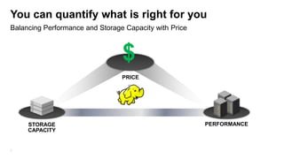
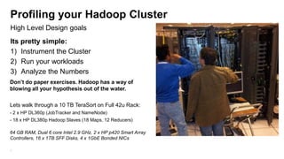
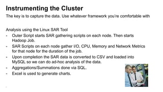
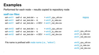
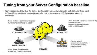
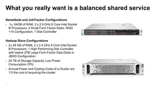
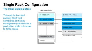
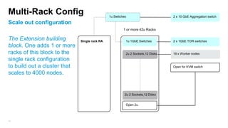
Taking the guesswork out of your
    Hadoop Infrastructure & O/S


      Steve Watt
      @wattsteve
      swatt@redhat.com
1
Agenda – Clearing up common misconceptions
                                 Web Scale Hadoop Origins
                                  Single/Dual Socket 1+ GHz
                                  4-8 GB RAM
                                  2-4 Cores
                                  1x 1GbE NIC
                                  (2-4) x 1 TB SATA Drives

                                 Commodity in 2013

                                  Dual Socket 2+ GHz
                                  24-48 GB RAM
                                  4-6 Cores
                                  (2-4) x 1GbE NICs
                                  (4-14) x 2 TB SATA Drives


                                  The enterprise
                                  perspective is also
                                  different
2
You can quantify what is right for you
Balancing Performance and Storage Capacity with Price


                                 $
                                 PRICE


     STORAGE                                            PERFORMANCE
     CAPACITY


3
“We’ve profiled our Hadoop
applications so we know what type
of infrastructure we need”
   Said no-one. Ever.
   (except Alan Wittenauer)
Profiling your Hadoop Cluster
High Level Design goals
Its pretty simple:
1) Instrument the Cluster
2) Run your workloads
3) Analyze the Numbers
Don’t do paper exercises. Hadoop has a way of
blowing all your hypothesis out of the water.

Lets walk through a 10 TB TeraSort on Full 42u Rack:
- 2 x HP DL360p (JobTracker and NameNode)
- 18 x HP DL380p Hadoop Slaves (18 Maps, 12 Reducers)

64 GB RAM, Dual 6 core Intel 2.9 GHz, 2 x HP p420 Smart Array
Controllers, 16 x 1TB SFF Disks, 4 x 1GbE Bonded NICs

5
Instrumenting the Cluster
The key is to capture the data. Use whatever framework you’re comfortable with


Analysis using the Linux SAR Tool
- Outer Script starts SAR gathering scripts on each node. Then starts
   Hadoop Job.
- SAR Scripts on each node gather I/O, CPU, Memory and Network Metrics
   for that node for the duration of the job.
- Upon completion the SAR data is converted to CSV and loaded into
   MySQL so we can do ad-hoc analysis of the data.
- Aggregations/Summations done via SQL.
- Excel is used to generate charts.


6
Examples
Performed for each node – results copied to repository node
sadf csv files:
    ssh wkr01   sadf -d sar_test.dat -- -u     > wkr01_cpu_util.csv            repos
    ssh wkr01   sadf -d sar_test.dat -- -b     > wkr01_io_rate.csv
    ssh wkr01   sadf -d sar_test.dat -- -n DEV > wkr01_net_dev.csv

    ssh wkr02   sadf -d sar_test.dat -- -u     > wkr02_cpu_util.csv
    ssh wkr02   sadf -d sar_test.dat -- -b     > wkr02_io_rate.csv    wkr01_cpu_util.csv
    ssh wkr02   sadf -d sar_test.dat -- -n DEV > wkr02_net_dev.csv    wkr01_io_rate.csv
    …                                                                 wkr01_net_dev.csv

    File name is prefixed with node name (i.e., “wrknn”)              wkr02_cpu_util.csv
                                                                      wkr02_io_rate.csv
                                                                      wkr02_net_dev.csv
7
I/O Subsystem Test Chart
I/O Subsystem has only around 10% of Total Throughput Utilization

                                                 RUN the DD Tests first to understand
                                                 what the Read and Write throughput
                                                 capabilities of your I/O Subsystem

                                                 -X axis is time
                                                 -Y axis is MB per second

                                                 TeraSort for this server design is not
                                                 I/O bound. 1.6 GB/s is upper bound,
                                                 this is less than 10% utilized.


8
Network Subsystem Test Chart
Network throughput utilization per server less than a ¼ of capacity

                                                 A 1GbE NICs can drive up to 1Gb/s for
                                                 Reads and 1Gb/s for Writes which is
                                                 roughly 4 Gb/s or 400 MB/s total across
                                                 all bonded NICs

                                                 -Y axis is throughput
                                                 -X axis is elapsed time

                                                 Rx = Received MB/sec
                                                 Tx = Transmitted MB/sec
                                                 Tot = Total MB/sec


9
CPU Subsystem Test Chart
CPU Utilization is High, I/O Wait is low – Where you want to be

                                              Each data point is taken every 30 seconds
                                              Y axis is percent utilization of CPUs
                                              X axis is timeline of the run

                                              CPU Utilization is captured by analyzing
                                              how busy each core is and creating an
                                              average

                                              IO Wait (1 of 10 other SAR CPU Metrics)
                                              measures percentage of time CPU is
                                              waiting on I/O


10
Memory Subsystem Test Chart
High Percentage Cache Ratio to Total Memory shows CPU is not waiting on
memory
                                          -X axis is Memory Utilization
                                          -Y axis is elapsed time

                                          -Percent Caches is a SAR Memory Metrics
                                          (kb_cached). Tells you how many blocks of
                                          memory are cached in the Linux Memory Page
                                          Cache. The amount of memory used to cache
                                          data by the kernel.

                                          -Means we’re doing a good job of caching data
                                          so the JVM is not having to do I/Os and
                                          incurring I/O wait time (reflected in the previous
                                          slide)


11
Tuning from your Server Configuration baseline
- We’ve established now that the Server Configuration we used works pretty well. But what if you want
  to Tune it? i.e. sacrifice some performance for cost or to remove an I/O, Network or Memory
  limitation?

     -Types of Disks / Controllers / Capacity                               - Type (Socket R 130 W vs. Socket B 95 W)
     -Number of Disks / RAID vs. JBOD                                       - Amount of Cores
                                                                            - Amount of Memory Channels
                                                                            - 4GB vs. 8GB DIMMS


           I/O SUBSYSTEM                                       COMPUTE


                                                                               - Type of Network
                                                                               - Amount of Server of NICs
                                                                               - Switch Port Availability
           DATA CENTER                                         NETWORK         - Deep Buffering
     -Floor Space (Rack Density)                SCALE
12   -Power and Cooling Constraints
Tpapi (Flickr)


13   Introducing Hadoop Ops whack-a-mole
What you really want is a balanced shared service
NameNode and JobTracker Configurations
- 1u, 64GB of RAM, 2 x 2.9 GHz 6 Core Intel Socket
  R Processors, 4 Small Form Factor Disks, RAID
  1+0 Configuration, 1 Disk Controller

Hadoop Slave Configurations
- 2u 48 GB of RAM, 2 x 2.4 GHz 6 Core Intel Socket
  B Processors, 1 High Performing Disk Controller
  with twelve 2TB Large Form Factor Data Disks in
  JBOD Configuration
- 24 TB of Storage Capacity, Low Power
  Consumption CPU
- Annual Power and Cooling Costs of a Cluster are
  1/3 the cost of acquiring the cluster


14
Single Rack Configuration
The Initial Building Block      42u rack enclosure


                               1u 1GbE Switches         2 x 1GbE TOR switches
This rack is the initial
building block that            1u 2 Sockets, 4 Disks    1 x Management node
configures all the key
management services for a      2u 2 Sockets, 12 Disks   1 x JobTracker node

production scale out cluster                            1 x Name node
to 4000 nodes.
                                                        (3-18) x Worker nodes


                                                        Open for KVM switch
                               2u 2 Sockets, 12 Disks


                               Open 1u


15
Multi-Rack Config                              1u Switches                       2 x 10 GbE Aggregation switch

Scale out configuration
                                                        1 or more 42u Racks

The Extension building        Single rack RA             1u 1GbE Switches        2 x 1GbE TOR switches
block. One adds 1 or more
racks of this block to the                               2u 2 Sockets,12 Disks   19 x Worker nodes
single rack configuration
to build out a cluster that                                                      Open for KVM switch

scales to 4000 nodes.


                                                         2u 2 Sockets,12 Disks


                                                         Open 2u


16
Linux Optimizations
Performance and High Availability

- Turn off caching on the controller

- RHEL 6.1, mount volumes with NOATIME setting, Disable Transparent
  HugePage compaction if using RHEL 6.2 or later.

- Optional NameNode HA with HA Kit for RHEL (3 NameNodes using
  Shared Storage and a Power Fencing Device)

- In the process of doing filesystem (EXT vs. XFS) analysis. Stay tuned.


17
System on a Chip and Hadoop
Intel ATOM and ARM Processor Server Cartridges
                                                   Hadoop has come full circle


                                                          4-8 GB RAM
                                                          4 Cores 1.8 GHz
                                                          2-4 TB
                                                          1 GbE NICs


                                                 - Amazing Density Advances. 270 +
                                                   servers in a Rack (compared to 21!).


                                                 - Trevor Robinson from Calxeda is a
                                                   member of our community working
                                                   on this. He’d love some help:
                                                   trevor.robinson@calxeda.com
18
Thanks to our partner HP for letting me present their findings. If
     you’re interested in learning more about these findings please check
     out hp.com/go/hadoop and see detailed reference architectures and
     varying server configurations for Hortonworks, MapR and Cloudera.

     Steve Watt   swatt@redhat.com @wattsteve


19
Backup


20
HBase Testing – Results still TBD
     YCSB Workload A and C unable to Drive the CPU
                     CPU Utilization                                                        Network Usage                    2 Workloads Tested:
             100                                                            300                                              - YCSB workload “C” : 100% read-
Axis Title


                                                                                                                             only requests, random access to


                                                                  MB/sec
                                                                            200
              50
                                                                            100                                              DB, using a unique primary key
                                                    %busy                                                        Tx MB/sec
               0                                                                        -                                    value
                                                    %iowait                                                      Rx MB/sec
                   1 3 5 7 9
                                                                                            1 4 7 10131619
                               11 13 15 17 19 21
                                                                                                                             - YCSB workload “A” : 50% read and
                                                                                               Minutes
                         Minutes                                                                                             50% updates, random access to DB,
                                                                                                                             using a unique primary key value

                         Disk Usage                                                            Memory Usage                  -When data is cached in HBase
             300                                                                        100                                  cache, performance is really good
MB/sec


                                                                           Axis Title
             200                                                                         50                                  and we can occupy the CPU. Ops
             100                                                                          0                       %memused   throughput (and hence CPU
               -                                   Write MB/sec
                                                                                              1 5 8                          Utilization) dwindles when data
                                                                                                      12 15 19    %cached
                    1 4 6 9                        Read MB/sec
                               11 14 16 19 21                                                                                exceeds HBase cache but is
                                                                                                 Minutes
                         Minutes                                                                                             available in Linux cache. Resolution
     21                                                                                                                      TBD – Related JIRA HDFS-2246

Optimizing your Infrastrucure and Operating System for Hadoop

  • 1.
    Taking the guessworkout of your Hadoop Infrastructure & O/S Steve Watt @wattsteve swatt@redhat.com 1
  • 2.
    Agenda – Clearingup common misconceptions Web Scale Hadoop Origins Single/Dual Socket 1+ GHz 4-8 GB RAM 2-4 Cores 1x 1GbE NIC (2-4) x 1 TB SATA Drives Commodity in 2013 Dual Socket 2+ GHz 24-48 GB RAM 4-6 Cores (2-4) x 1GbE NICs (4-14) x 2 TB SATA Drives The enterprise perspective is also different 2
  • 3.
    You can quantifywhat is right for you Balancing Performance and Storage Capacity with Price $ PRICE STORAGE PERFORMANCE CAPACITY 3
  • 4.
    “We’ve profiled ourHadoop applications so we know what type of infrastructure we need” Said no-one. Ever. (except Alan Wittenauer)
  • 5.
    Profiling your HadoopCluster High Level Design goals Its pretty simple: 1) Instrument the Cluster 2) Run your workloads 3) Analyze the Numbers Don’t do paper exercises. Hadoop has a way of blowing all your hypothesis out of the water. Lets walk through a 10 TB TeraSort on Full 42u Rack: - 2 x HP DL360p (JobTracker and NameNode) - 18 x HP DL380p Hadoop Slaves (18 Maps, 12 Reducers) 64 GB RAM, Dual 6 core Intel 2.9 GHz, 2 x HP p420 Smart Array Controllers, 16 x 1TB SFF Disks, 4 x 1GbE Bonded NICs 5
  • 6.
    Instrumenting the Cluster Thekey is to capture the data. Use whatever framework you’re comfortable with Analysis using the Linux SAR Tool - Outer Script starts SAR gathering scripts on each node. Then starts Hadoop Job. - SAR Scripts on each node gather I/O, CPU, Memory and Network Metrics for that node for the duration of the job. - Upon completion the SAR data is converted to CSV and loaded into MySQL so we can do ad-hoc analysis of the data. - Aggregations/Summations done via SQL. - Excel is used to generate charts. 6
  • 7.
    Examples Performed for eachnode – results copied to repository node sadf csv files: ssh wkr01 sadf -d sar_test.dat -- -u > wkr01_cpu_util.csv repos ssh wkr01 sadf -d sar_test.dat -- -b > wkr01_io_rate.csv ssh wkr01 sadf -d sar_test.dat -- -n DEV > wkr01_net_dev.csv ssh wkr02 sadf -d sar_test.dat -- -u > wkr02_cpu_util.csv ssh wkr02 sadf -d sar_test.dat -- -b > wkr02_io_rate.csv wkr01_cpu_util.csv ssh wkr02 sadf -d sar_test.dat -- -n DEV > wkr02_net_dev.csv wkr01_io_rate.csv … wkr01_net_dev.csv File name is prefixed with node name (i.e., “wrknn”) wkr02_cpu_util.csv wkr02_io_rate.csv wkr02_net_dev.csv 7
  • 8.
    I/O Subsystem TestChart I/O Subsystem has only around 10% of Total Throughput Utilization RUN the DD Tests first to understand what the Read and Write throughput capabilities of your I/O Subsystem -X axis is time -Y axis is MB per second TeraSort for this server design is not I/O bound. 1.6 GB/s is upper bound, this is less than 10% utilized. 8
  • 9.
    Network Subsystem TestChart Network throughput utilization per server less than a ¼ of capacity A 1GbE NICs can drive up to 1Gb/s for Reads and 1Gb/s for Writes which is roughly 4 Gb/s or 400 MB/s total across all bonded NICs -Y axis is throughput -X axis is elapsed time Rx = Received MB/sec Tx = Transmitted MB/sec Tot = Total MB/sec 9
  • 10.
    CPU Subsystem TestChart CPU Utilization is High, I/O Wait is low – Where you want to be Each data point is taken every 30 seconds Y axis is percent utilization of CPUs X axis is timeline of the run CPU Utilization is captured by analyzing how busy each core is and creating an average IO Wait (1 of 10 other SAR CPU Metrics) measures percentage of time CPU is waiting on I/O 10
  • 11.
    Memory Subsystem TestChart High Percentage Cache Ratio to Total Memory shows CPU is not waiting on memory -X axis is Memory Utilization -Y axis is elapsed time -Percent Caches is a SAR Memory Metrics (kb_cached). Tells you how many blocks of memory are cached in the Linux Memory Page Cache. The amount of memory used to cache data by the kernel. -Means we’re doing a good job of caching data so the JVM is not having to do I/Os and incurring I/O wait time (reflected in the previous slide) 11
  • 12.
    Tuning from yourServer Configuration baseline - We’ve established now that the Server Configuration we used works pretty well. But what if you want to Tune it? i.e. sacrifice some performance for cost or to remove an I/O, Network or Memory limitation? -Types of Disks / Controllers / Capacity - Type (Socket R 130 W vs. Socket B 95 W) -Number of Disks / RAID vs. JBOD - Amount of Cores - Amount of Memory Channels - 4GB vs. 8GB DIMMS I/O SUBSYSTEM COMPUTE - Type of Network - Amount of Server of NICs - Switch Port Availability DATA CENTER NETWORK - Deep Buffering -Floor Space (Rack Density) SCALE 12 -Power and Cooling Constraints
  • 13.
    Tpapi (Flickr) 13 Introducing Hadoop Ops whack-a-mole
  • 14.
    What you reallywant is a balanced shared service NameNode and JobTracker Configurations - 1u, 64GB of RAM, 2 x 2.9 GHz 6 Core Intel Socket R Processors, 4 Small Form Factor Disks, RAID 1+0 Configuration, 1 Disk Controller Hadoop Slave Configurations - 2u 48 GB of RAM, 2 x 2.4 GHz 6 Core Intel Socket B Processors, 1 High Performing Disk Controller with twelve 2TB Large Form Factor Data Disks in JBOD Configuration - 24 TB of Storage Capacity, Low Power Consumption CPU - Annual Power and Cooling Costs of a Cluster are 1/3 the cost of acquiring the cluster 14
  • 15.
    Single Rack Configuration TheInitial Building Block 42u rack enclosure 1u 1GbE Switches 2 x 1GbE TOR switches This rack is the initial building block that 1u 2 Sockets, 4 Disks 1 x Management node configures all the key management services for a 2u 2 Sockets, 12 Disks 1 x JobTracker node production scale out cluster 1 x Name node to 4000 nodes. (3-18) x Worker nodes Open for KVM switch 2u 2 Sockets, 12 Disks Open 1u 15
  • 16.
    Multi-Rack Config 1u Switches 2 x 10 GbE Aggregation switch Scale out configuration 1 or more 42u Racks The Extension building Single rack RA 1u 1GbE Switches 2 x 1GbE TOR switches block. One adds 1 or more racks of this block to the 2u 2 Sockets,12 Disks 19 x Worker nodes single rack configuration to build out a cluster that Open for KVM switch scales to 4000 nodes. 2u 2 Sockets,12 Disks Open 2u 16
  • 17.
    Linux Optimizations Performance andHigh Availability - Turn off caching on the controller - RHEL 6.1, mount volumes with NOATIME setting, Disable Transparent HugePage compaction if using RHEL 6.2 or later. - Optional NameNode HA with HA Kit for RHEL (3 NameNodes using Shared Storage and a Power Fencing Device) - In the process of doing filesystem (EXT vs. XFS) analysis. Stay tuned. 17
  • 18.
    System on aChip and Hadoop Intel ATOM and ARM Processor Server Cartridges Hadoop has come full circle 4-8 GB RAM 4 Cores 1.8 GHz 2-4 TB 1 GbE NICs - Amazing Density Advances. 270 + servers in a Rack (compared to 21!). - Trevor Robinson from Calxeda is a member of our community working on this. He’d love some help: trevor.robinson@calxeda.com 18
  • 19.
    Thanks to ourpartner HP for letting me present their findings. If you’re interested in learning more about these findings please check out hp.com/go/hadoop and see detailed reference architectures and varying server configurations for Hortonworks, MapR and Cloudera. Steve Watt swatt@redhat.com @wattsteve 19
  • 20.
  • 21.
    HBase Testing –Results still TBD YCSB Workload A and C unable to Drive the CPU CPU Utilization Network Usage 2 Workloads Tested: 100 300 - YCSB workload “C” : 100% read- Axis Title only requests, random access to MB/sec 200 50 100 DB, using a unique primary key %busy Tx MB/sec 0 - value %iowait Rx MB/sec 1 3 5 7 9 1 4 7 10131619 11 13 15 17 19 21 - YCSB workload “A” : 50% read and Minutes Minutes 50% updates, random access to DB, using a unique primary key value Disk Usage Memory Usage -When data is cached in HBase 300 100 cache, performance is really good MB/sec Axis Title 200 50 and we can occupy the CPU. Ops 100 0 %memused throughput (and hence CPU - Write MB/sec 1 5 8 Utilization) dwindles when data 12 15 19 %cached 1 4 6 9 Read MB/sec 11 14 16 19 21 exceeds HBase cache but is Minutes Minutes available in Linux cache. Resolution 21 TBD – Related JIRA HDFS-2246

Editor's Notes

  • #3  The average enterprise customers are running 1 or 2 Racks in Production. In that scenario, you have redundant switches in each RACK and you RAID Mirror the O/S and Hadoop Runtime and JBOD the Data Drives because losing Racks and Servers is costly. VERY Different to the Web Scale perspective.
  • #4 Hadoop Slave Server Configurations are about balancing the following: Performance (Keeping the CPU as busy as possible) Storage Capacity (Important for HDFS) Price (Managing the above at a price you can afford)Commodity Servers do not mean cheap. At scale you want to fully optimize performance and storage capacity for your workloads to keep costs down.
  • #5 So as any good Infrastructure Designer will tell you… you begin by Profiling your Hadoop Applications.
  • #11 But generally speaking, you design a pretty decent cluster infrastructure baseline that you can later optimize, provided you get these things right.
  • #15 In reality, you don’t want Hadoop Clusters popping up all over the place in your company. It becomes untenable to manage. You really want a single large cluster managed as a service.If that’s the case then you don’t want to be optimizing your cluster for just one workload, you want to be optimizing this for multiple concurrent workloads (dependent on scheduler) and have a balanced cluster.