Downloaded 44 times


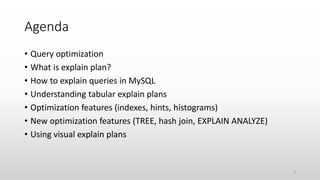
![How to explain queries - EXPLAIN syntax
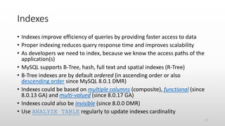
• The general syntax is:
{EXPLAIN | DESCRIBE | DESC}
[explain_type: {FORMAT = {TRADITIONAL | JSON | TREE}]
{statement | FOR CONNECTION con_id}
• Statement could be SELECT, DELETE, INSERT, REPLACE or UPDATE
(before 5.6.3 only SELECT)
• TREE is new format since 8.0.16 GA (2019-04-25)
• Can explain the currently executing query for a connection (since 5.7.2)
• Requires SELECT privilege for tables and views + SHOW VIEW privilege for
views
• DESCRIBE is synonym for EXPLAIN but used mostly for getting table
structure
7](https://image.slidesharecdn.com/optimizingqueriesinmysql-191118120344/85/Optimizing-queries-MySQL-7-320.jpg)
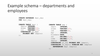
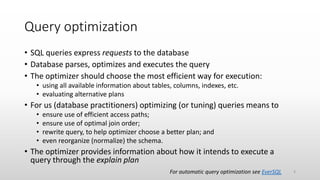
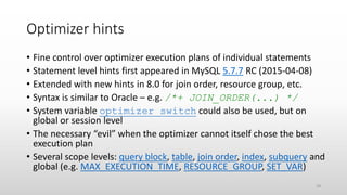
![Understanding tabular explain plans 1/5
• id: the sequential number of the SELECT in
query
• select_type: possible values include:
+----+-------------+
| id | select_type |
+----+-------------+
| 1 | SIMPLE |
| 1 | SIMPLE |
+----+-------------+
Value Meaning
SIMPLE no unions or subqueries
PRIMARY outermost SELECT
[DEPENDENT] UNION [dependent on outer query] second or later SELECT in a union
UNION RESULT result of a union
[DEPENDENT] SUBQUERY [dependent on outer query] first SELECT in subquery
[DEPENDENT] DERIVED [dependent on another table] derived table
MATERIALIZED materialized subquery
UNCACHEABLE [SUBQUERY|UNION] a subquery/union that must be re-evaluated for each row of the outer query
11](https://image.slidesharecdn.com/optimizingqueriesinmysql-191118120344/85/Optimizing-queries-MySQL-11-320.jpg)
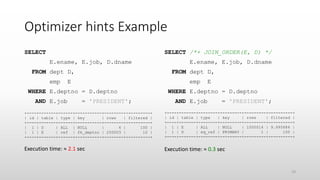
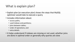
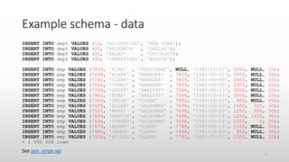
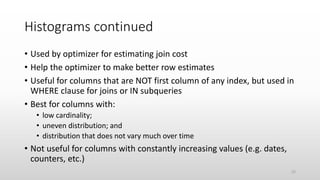
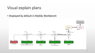
![Histogram types
Singleton
• Single value per bucket
• Bucket stores value and cumulative
frequency
• Useful for estimation of equality and
range conditions
Equi-height
• Multiple values per bucket
• Bucket stores min and max inclusive
values, cumulative frequency and
number of distinct values
• Frequent values in separate buckets
• Most useful for range conditions
21
0
0.1
0.2
0.3
0.4
0.5
0.6
5 4 3 1 2
Frequency
0
0.05
0.1
0.15
0.2
0.25
0.3
[1,7] 8 [9,12] [13,19] [20,25]
[1,7] 8 [9,12] [13,19] [20,25]](https://image.slidesharecdn.com/optimizingqueriesinmysql-191118120344/85/Optimizing-queries-MySQL-21-320.jpg)
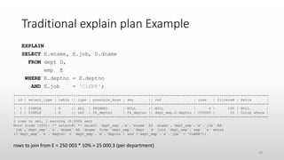
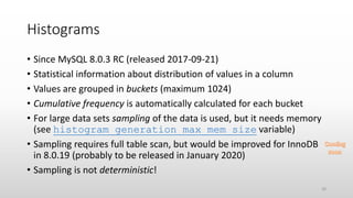
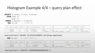
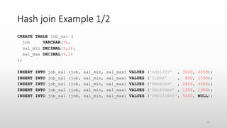
![Histogram Example 1/4 – creation and meta
ANALYZE TABLE emp
UPDATE HISTOGRAM ON job
WITH 5 BUCKETS;
{"buckets": [
["base64:type254:QU5BTFlTVA==", 0.44427638528762128],
["base64:type254:Q0xFUks=" , 0.7765828956408041],
["base64:type254:TUFOQUdFUg==", 0.8882609755557034],
["base64:type254:U0FMRVNNQU4=", 1.0]
],
"data-type": "string",
"null-values": 0.0,
"collation-id": 33,
"last-updated": "2019-10-17 07:33:42.007222",
"sampling-rate": 0.10810659461578348,
"histogram-type": "singleton",
"number-of-buckets-specified": 5
}
SELECT JSON_PRETTY(`histogram`)
FROM INFORMATION_SCHEMA.COLUMN_STATISTICS CS
WHERE CS.`schema_name` = 'dept_emp'
AND CS.`table_name` = 'emp'
AND CS.`column_name` = 'job';
23](https://image.slidesharecdn.com/optimizingqueriesinmysql-191118120344/85/Optimizing-queries-MySQL-23-320.jpg)
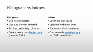
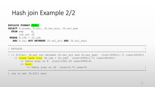
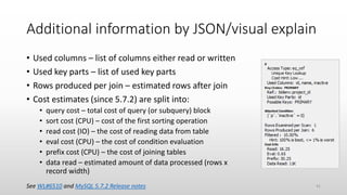
![Histogram Example 2/4 - sampling
SET histogram_generation_max_mem_size = 184*1024*1024; /* 184 MB */
ANALYZE TABLE emp UPDATE HISTOGRAM ON job WITH 5 BUCKETS;
{"buckets": [
["base64:type254:QU5BTFlTVA==", 0.4440377834710314],
["base64:type254:Q0xFUks=" , 0.777311117644353],
["base64:type254:TUFOQUdFUg==", 0.8887915569182032],
["base64:type254:UFJFU0lERU5U", 0.8887925569042035],
["base64:type254:U0FMRVNNQU4=", 1.0]
],
"data-type": "string",
"null-values": 0.0,
"collation-id": 33,
"last-updated": "2019-10-21 10:52:03.974566",
"sampling-rate": 1.0,
"histogram-type": "singleton",
"number-of-buckets-specified": 5
}
Note: Setting histogram_generation_max_mem_size requires SESSION_VARIABLES_ADMIN (since 8.0.14) or
SYSTEM_VARIABLES_ADMIN privilege. 24](https://image.slidesharecdn.com/optimizingqueriesinmysql-191118120344/85/Optimizing-queries-MySQL-24-320.jpg)
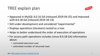
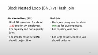
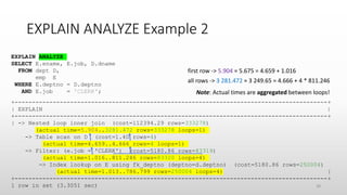
![Histogram Example 3/4 - frequencies
SELECT HG.val, ROUND(HG.freq, 3) cfreq,
ROUND(HG.freq - LAG(HG.freq, 1, 0) OVER (), 3) freq
FROM INFORMATION_SCHEMA.COLUMN_STATISTICS CS,
JSON_TABLE(`histogram`->'$.buckets', '$[*]'
COLUMNS(val VARCHAR(10) PATH '$[0]',
freq DOUBLE PATH '$[1]')) HG
WHERE CS.`schema_name` = 'dept_emp'
AND CS.`table_name` = 'emp'
AND CS.`column_name` = 'job';
+-----------+-------+-------+
| val | cfreq | freq |
+-----------+-------+-------+
| ANALYST | 0.444 | 0.444 |
| CLERK | 0.777 | 0.333 |
| MANAGER | 0.889 | 0.111 |
| PRESIDENT | 0.889 | 0 |
| SALESMAN | 1 | 0.111 |
+-----------+-------+-------+
5 rows in set (0.0009 sec)
25](https://image.slidesharecdn.com/optimizingqueriesinmysql-191118120344/85/Optimizing-queries-MySQL-25-320.jpg)
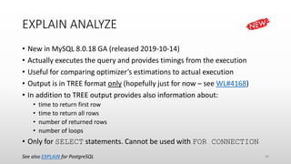
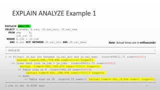
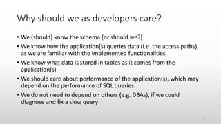
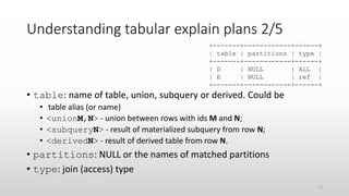
![Problems with TREE and EXPLAIN ANALYZE
• Will not explain queries using nested loop (shows just “not executable
by iterator executor”)
• Will not explain SELECT COUNT(*) FROM table queries (shows
just “Count rows in table”)
• Does not compute select list subqueries (see bug 97296) [FIXED]
• Not integrated with MySQL Workbench (see bug 97282)
• Does not print units on timings (see bug 97492)
39](https://image.slidesharecdn.com/optimizingqueriesinmysql-191118120344/85/Optimizing-queries-MySQL-39-320.jpg)
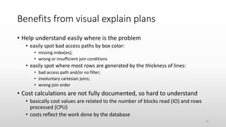


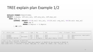
The document discusses optimizing queries in MySQL, including the use of explain plans to understand execution paths, the importance of indexing, and new optimization features. It emphasizes the developer's role in query performance and outlines the syntax for using explain plans, as well as the types of information they provide. Additionally, it covers topics such as optimizer hints, histograms, and the various types of indexes that can be used to improve query efficiency.