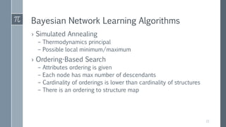
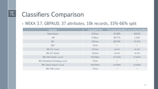
This document discusses optimal Bayesian networks for classification problems. It covers Bayesian network concepts like DAGs, CPTs, and probability inference. Naive Bayes and Bayesian network classifiers are presented with examples. Learning Bayesian networks from data is discussed, including structure and parameter learning algorithms like K2, hill climbing, simulated annealing, and TAN. Computational challenges like combinatorial optimization and feature selection are addressed. Comparisons of classifier performance on real datasets demonstrate Bayesian networks can achieve high accuracy.

1. Optimal Bayesian Networks
Advanced Topics in Computer Science Seminar
Supervisor: Dr. Herman Maya
Author: Kreimer Andrew
1

2. Data Mining
› Massive amounts of data: Petabyte, Terabyte
› Data evolution
› Multidisciplinary field
› Data Warehouse
› OLAP & OLTP
› Preprocessing
› KDD – Knowledge Discovery in Databases
› One truth
2

3. Data Mining Methods
› Clustering
– Bank clients: private or business
› Association Rules
– YouTube suggestions, Amazon checkout suggestions
› Classification and Prediction
– SPAM mail classification, FX trend predictions
– Payment power prediction
› Integration
– Clustered client gets specific classification model
3

4. The Bayesian Approach
› Probability & Statistics
– Instances – classical approach
– A priori/A posteriori knowledge – the Bayesian approach
› Bayes’ Theorem
– P(A|B) = P(B|A)P(A)/P(B)
› MAP
– Maximum A Posteriori
– 𝑨 𝑴𝑨𝑷 = 𝐚𝐫𝐠 𝒎𝒂𝒙 𝑨 𝑷 𝑨 𝑩 = 𝐚𝐫𝐠 𝒎𝒂𝒙 𝑨 𝑷 𝑩 𝑨 𝑷(𝑨)
4

5. Bayesian Classifier
› Describe a client by age and income
› P(X) – probability that exists a client aged 25 with income of
5000
› P(H) – probability that client buys a guitar
› P(X|H) – probability that exists client X given that someone
bought a guitar
› P(H|X) – probability of client X buying a guitar
› P(H|X) = P(X|H)P(H)/P(X)
› The Naïve approach
– Independent variables
5

6. Naïve Bayes Classifier
› Optimal classifier is not practical
› The variables are independent
› Probability 0
– Laplace – add one dummy record
– m-estimate – there are m virtual records
6

7. Classification example using Naïve Bayes Classifier
News in EU News in US EU GDP US GDP EURUSD
bad bad Up Down Up
bad good Down Down Up
good bad Up Up Down
good good Up Up Up
bad bad Down Up Down
good bad Down Up Down
bad good Up Down Up
bad bad Up Down Down
good good Up Up Up
Bad good Down down Up
NewsEu, NewsUs ϵ {bad, good}
EuGDP, UsGDP, EURUSD (Class) ϵ {up, down}
Let’s try to classify trends in the FX market using several attributes: news in Europe, news in US, GDP in
Europe and news in US. Each instance is monthly measurement. News attributes describe general
market temperament. GDP attributes describe the change relative to last period.
7

8. Classification example using Naïve Bayes Classifier
› Let’s classify new instance
– X=(NewsEU = good, NewsUS = bad, EuGDP = up, UsGDP = up)
› We start with 𝑷 𝑿 𝑪𝒊 𝑷(𝑪𝒊) :
– 𝑷 𝑪𝒊 :
– P(EURUSD = Up) = 6/10 = 0.6
– P(EURUSD = Down) = 4/10 = 0.4
› Then we calculate the joints
– 𝑷 𝑿𝒋|𝑪𝒊 :
– P(NewsEu = good | EURUSD = Up) = 2/6 = 0.33
– P(NewsUs = bad | EURUSD = Up) = 1/6 = 0.16
– etc.
8

9. Classification example using Naïve Bayes Classifier
› The classification:
› 𝑷 𝑿|𝑪𝒊 :
› P(X|EURUSD = up) = P(NewsEu = good | EURUSD = up) * P(NewsUs = bad | EURUSD =
up) * P(EuGDP = up | EURUSD = up) * P(UsGDP = up | EURUSD = up) = 0.33 * 0.16 * 0.66
* 0.33 = 0.01149984
› P(X|EURUSD = down) = P(NewsEu = good | EURUSD = down) * P(NewsUs = bad |
EURUSD = down) * P(EuGDP = up | EURUSD = down) * P(UsGDP = up | EURUSD = down)
= 0.5 * 1 * 0.5 * 0.75 = 0.1875
› Using MAP:
› 𝒉 𝑴𝑨𝑷= max{P(X|EURUSD=up)P(EURUSD=up), P(X|EURUSD=down)P(EURUSD=down)} =
max{0.01149984, 0.1875} = 0.1875
› Conclusion: trend down, we should sell EURUSD.
9

10. Bayesian Network
› Graphical probabilistic model
› DAG
› CPT for each attribute
› d-separated ,d-connected
› A -> D, D -> A
› P(C|A,B,D,E) = P(C|A,B,D)
– E and C are d-separated
10

11. Probability Inference
› Probability calculation:
– 𝑷 𝒙 𝟏, 𝒙 𝟐, … , 𝒙 𝒏 = 𝒊=𝟏
𝒏
𝑷(𝒙𝒊|𝑷𝒂𝒓𝒆𝒏𝒕𝒔 𝒀𝒊 )
› Given A, B, C, D & E, calculate P(A, B, C, D, E):
– 𝑷 𝑨, 𝑩, 𝑪, 𝑫, 𝑬 = 𝑷 𝑨 ∗ 𝑩 𝑨 ∗ 𝑷 𝑪 𝑨, 𝑩, 𝑫 ∗ 𝑷 𝑫 𝑨, 𝑫
∗ 𝑷 𝑬 𝑨, 𝑩, 𝑪, 𝑫
› Given A, B, D & E, calculate C by using MAP:
– 𝑷 𝑪 𝑨, 𝑩, 𝑫, 𝑬 = 𝒉 𝑴𝑨𝑷(𝑷 𝑪 𝑨, 𝑩, 𝑫 , 𝑷 ¬𝑪 𝑨, 𝑩, 𝑫 ) = 𝑷 ¬𝑪 𝑨, 𝑩, 𝑫
– if 𝑷 𝑪 𝑨, 𝑩, 𝑫 > 𝑷 ¬𝑪 𝑨, 𝑩, 𝑫 then 𝑪 else ¬𝑪
› Given A, C, D & E, calculate B by using Bayes Theorem:
– P(A|B) = P(B|A) * P(A)/P(B) //Bayes Theorem
– P(B) = P(B|A) + P(B|^A) = P(B|A) * P(A) + P(B|^A) * P(^A) = …
11

12. Dynamic Bayesian Network
› Bayesian Network extension
› Time slice attributes relations
› Matrix of attributes and time slices
› Time series
› Cycle are allowed
› 𝑿 𝟏 → 𝑿 𝟐 → ⋯ → 𝑿 𝒏 X1
X2
X3
X4Attribute p…Attribute 2Attribute 1
𝑿 𝟏𝒑…𝑿 𝟏𝟐𝑿 𝟏𝟏Time 1
𝑿 𝟐𝒑…𝑿 𝟐𝟐𝑿 𝟐𝟏Time 2
……………
𝑿 𝒏𝒑…𝑿 𝒏𝟐𝑿 𝒏𝟏Time n
12

13. Bayesian Network Example
› Let’s try to predict trends in EURUSD
› Binary class variable: Up or Down
› Attributes: Open, High, Low, Close, MA100, MA200
› Class: ClassTrend
13

14. Bayesian Network Example
CPT: BN:
14

15. Bayesian Network Learning
› Structure is given by field expert (Wish You Were Here)
› Structure learning - computational barrier
– 2 𝑛 structures
– Heuristics
– Metrics for evaluating structures: local, global, d-separation
› Conditional Probability Tables calculation
15

16. Bayesian Network Learning
› Attributes ordering:
– Set {𝑋1, 𝑋2, … , 𝑋 𝑛}
– 𝑋𝑖 is candidate parent of 𝑋𝑗 iff 𝑋𝑖 is before 𝑋𝑗 in order
– Possible parents come before the node in order
› Structure
– DAG
X1 X3 X2
X1
X3X2
Order(left) and Structure(right)
16

17. Network Scoring
› Structures are evaluated by scoring (global/local)
› Bayesian Dirichlet – BD
› BDeu (equivalent uniform Bayesian Dirichlet).
› 𝐴𝐼𝐶 𝐴𝑘𝑎𝑖𝑘𝑒′ 𝑠 𝐼𝑛𝑓𝑜𝑟𝑚𝑎𝑡𝑖𝑜𝑛 𝐶𝑟𝑖𝑡𝑒𝑟𝑖𝑜𝑛 → 𝑓 𝑁 = 1
› 𝐵𝐼𝐶 𝐵𝑎𝑦𝑒𝑠𝑖𝑎𝑛 𝐼𝑛𝑓𝑜𝑟𝑚𝑎𝑡𝑖𝑜𝑛 𝐶𝑟𝑖𝑡𝑒𝑟𝑖𝑜𝑛 → 𝑓 𝑁 =
1
2
𝑙𝑜𝑔𝑁
› MDL given model M and dataset D:
– Description cost: 𝐶𝑜𝑠𝑡 𝑀 + 𝐶𝑜𝑠𝑡 𝐷 𝑀
– Looking for minimum or maximum (start at −∞)
17

18. Bayesian Network Learning Algorithms
› Gradient Descent
– Structure is given, CPT to be calculated
– Some of the a priori probabilities are missing
– Infinitesimal approximation
› K2
– Well known
– Greedy Algorithm
– Each node has a maximum number of parents
– Add parents gradually (from 0)
– Attributes ordering is given
– Look for the structure having highest score
– Stop when no better structure is found
18

19. Bayesian Network Learning Algorithms
› Hill-Climbing Search
– Local Search, Global Search
– Global: incremental solution construction
– Local: start with random solution, optimize towards the optimal
1
4
8......8765
4
33
2
21
Global (right) vs. Local (left)
19

20. Bayesian Network Learning Algorithms
› Taboo Search
– List of forbidden solutions
– Allow bad solutions to reveal good solutions
– Avoid local max/min
– Efficient data structures
– Decisions made with 4 dimensions:
› Past occurrences
› Frequencies
› Quality
› Impact
Possible
Solutions
Solutions
Evaluation
Find Optimal
Solution
Stop?
Update
Taboo List
Initial
Solution
Optimal
Solution
Taboo Search scheme 20

21. Bayesian Network Learning Algorithms
› TAN – Tree Augmented Naïve Bayes
– Tree based
– Conditional Mutual Information
– Edges from class to attributes
– Chow-Liu (1968)
› ‫גנטי‬ ‫(אלגוריתם‬GA)
– Evolution
– Mutation
– Selection from several generations
Stop?
Selection
Solutions
Creation
New
Solutions
Change
Solution
Generation
Genetic Algorithm, Source: P. Larranaga et al.
Optimal
Solution
Initialization
21

22. Bayesian Network Learning Algorithms
› Simulated Annealing
– Thermodynamics principal
– Possible local minimum/maximum
› Ordering-Based Search
– Attributes ordering is given
– Each node has max number of descendants
– Cardinality of orderings is lower than cardinality of structures
– There is an ordering to structure map
22

23. Classifiers Comparison
› WEKA 3.6, votes.arff, 435 records, 17 attributes, 10 folds
FNTNFPTPInaccurateAccurate
Calculation
Time
Classifier
14154292389.89%90.11%0.01secNaïve Bayes
816082593.68%96.32%0secJ48
10158232447.59%92.41%0secIB1
10158132545.29%94.71%1.75secMLP
14154292389.89%90.11%0.04secBN, K2, Local
14154292389.89%90.11%0.01secBN, K2, Global
14154282399.66%90.34%0.02secBN, Hill Climber, Local
12156122555.52%94.48%2.87secBN, Hill Climber, Global
10158122555.06%94.94%1.34secBN, Simulated Annealing, Local
13155132545.98%94.02%52.04secBN, Simulated Annealing, Global
14154282399.66%90.34%0.02secBN, Taboo Search, Local
15153122556.21%93.79%1.92secBN, Taboo Search, Global
9159132545.06%94.94%0.04secBN, TAN, Local
6162152524.83%95.17%3.24secBN, TAN, Global 23

24. Classifiers Comparison
› WEKA 3.7, GBPAUD, 37 attributes, 10k records, 33%-66% split
Incorrectly ClassifiedCorrectly ClassifiedCalculatioT timeClassifier
36.62%63.38%0.03secNaïve Bayes
1.23%98.77%0.48secJ48
31.21%68.79%0.01secIB1
??>5minMLP
35.73%64.27%0.11secBN, K2, Local
35.73%64.27%3.62secBN, K2, Global
37.2647%62.7353%143.19secBN, Hill Climber, Local
??>5minBN, Simulated Annealing, Local
35.5294%64.4706%144.19minBN, Taboo Search, Local
??>5minBN, TAN, Local
24

25. Optimal Bayesian Network
› Combinatorial optimization
› Inference is difficult if we must visit the whole structure
› Curse of dimensionality
› Feature selection – critical phase
› Attributes ordering – usually must be calculated
› Search space pruning by heuristics
› A priori knowledge, field experts (Wish You Were Here)
25

26. Summary
› Graphical classification model
– Judea Pearl (1988)
– Chow-Liu (1968)
› Easily fitted
› Easily interpreted
› Computational limit (as always!)
› Polynomial algorithms?
– Time
– Memory
26

27. That's all folks!
Kreimer Andrew
Algonell.com – Scientific FX Trading
kreimer.andrew.@gmail.com
27