Download as PDF, PPTX

![Introduction Streamline Approach Heuristics Validation Summary End
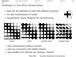
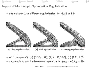
The Founding Papers in Topology Optimization
Bendsøe & Kikuchi; 1988; Generating optimal topologies in
optimal design using a homogenization method (3281 cites)
homogenized material [c] = H(s1,s2,θ)
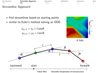
two-scale approach
see also talk by Th. Guess, M. Stingl, F. Wein
s2
s1
Bendsøe; 1989; Optimal shape design as a material distribution
problem (1375 cites)
single variable ρ scales homogeneous material
→ Solid Isotropic Material with Penalization
Fabian Wein Streamline interpretation of microstructures](https://image.slidesharecdn.com/opti14-140630033724-phpapp01/85/Interpretation-of-local-oriented-microstructures-by-a-streamline-approach-to-obtain-manufacturable-structures-2-320.jpg)

![Introduction Streamline Approach Heuristics Validation Summary End
Numerical Validation - Parameter Study
vary hs2 ∈ [10,40] and smin ∈ [0.01,0.2] → image → mesh → FEM
fixed hs1 = 40 and tmax = 2
10
20
30
40 0.0
0.1
0.2
0.210
0.215
0.220
0.225
0.230
vtotal
hs2
smin
vtotal
10
20
30
40 0.0
0.1
0.2
1.0
2.0
3.0
4.0
5.0 u
T
f
hs2
smin
u
T
f
minimal too low: many thin lines → vtotal cannot be reached
minimal too high: loose information → poor compliance
u f : homogenized=1.51, streamline ≈ 1.55 . . . 2.0, SIMP=1.13
Fabian Wein Streamline interpretation of microstructures](https://image.slidesharecdn.com/opti14-140630033724-phpapp01/85/Interpretation-of-local-oriented-microstructures-by-a-streamline-approach-to-obtain-manufacturable-structures-10-320.jpg)
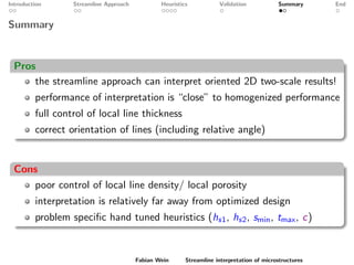
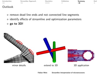
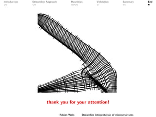

The document discusses a streamline approach to interpret optimized two-scale microstructures for manufacturing. It generates streamlines based on a material density field to represent oriented material distributions. Several heuristics are explored to control the line thickness and density. Numerical validation shows the approach can achieve similar compliance as homogenization while allowing control over manufacturing features. Further work is needed to improve local density control and extend the method to 3D microstructures.