Online Maths Assignment Help

For Any Assignment related queries, Call us at : - +1 678 648 4277
You can mail us at : - info@mathsassignmenthelp.com or
reach us at : - https://www.mathsassignmenthelp.com/

Problem 1 : Modified inner products for column vectors
Consider the inner product (x, y) = x∗By from class (lecture 5.5 notes), where the
vectors are in CN and B is an N × N Hermitian positive-definite matrix.
(a) Show that this inner product satisfies the required properties of inner products
from class: (x, y) = (y, x), (x, x) > 0 except for x = 0. (Linearity (x, αy+z) = α(x,
y)+(x, z) is obvious from linearity the of matrix operations; you need not show it.)
(b) If M is an arbitrary (possibly complex) N × N matrix, define the adjoint M† by (x,
My) = (M† x, y) (for all x, y). (In this problem, we use † instead of ∗ for the
adjoint in order to avoid confusion with the conjugate transpose: for this inner
product, the adjoint MT is not the conjugate transpose M∗ = MT .) Give an explicit
formula for M† in terms of M and B .
(c) Using your formula from above, show that M† = M (i.e., M is self-
adjoint/Hermitian for this inner product) if M = B−1A for some A = A∗ .
Problem 2: Finite-difference approximations
For this question you may find it helpful to refer to the notes and readings from lecture
3. Suppose that we want to compute the operation
mathsassignmenthelp.com

for some smooth function c(x) (you can assume c has a convergent Taylor series
everywhere). Now, we want to construct a finite-difference approximation for Aˆ with
u(x) on Ω = [0, L] and Dirichlet boundary conditions u(0) = u(L) = 0, similar to class,
approximating u(mΔx) ≈ um for M equally spaced points m = 1, 2, . . . , M, u0 =
uM+1 = 0, and Δx =
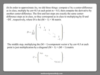
(a) Using center-difference operations, construct a finite-difference approximation for
Au ˆ evaluated at mΔx. (Hint: use a centered first-derivative evaluated at grid
points m + 0.5, as in class, followed by multiplication by c, followed by another
centered first derivative. Do not ′ ′ ′′ separate Au ˆ by the product rule into c’ u’ +
cu” first, as that will make the factorization in part (d) more difficult.)
(b) Show that your finite-difference expressions correspond to approximating Au ˆ by
Au where u is the column vector of the M points um and A is a real-symmetric
matrix of the form A = −DTCD (give C, and show that D is the same as the 1st-
derivative matrix from lecture).

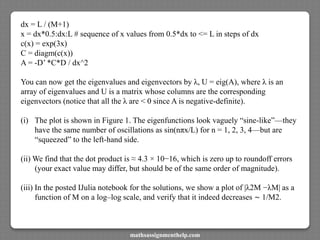
(c) In Julia, the diagm(c) command will create a diagonal matrix from a vector c. The
function diff1(M) = [ [1.0 zeros(1,M-1)]; diagm(ones(M-1),1) - eye(M) ] will allow
you to create the (M + 1)×M matrix D from class via D = diff1(M) for any given value
of M. Using these two commands, construct the matrix A from part (d) for M = 100 and
L = 1 and c(x) = e3x via
L = 1
M = 100
D = diff1(M)
dx = L / (M+1)
x = dx*0.5:dx:L # sequence of x values from 0.5*dx to <= L in steps of dx
C = ....something from c(x)...hint: use diagm...
A = -D’ * C * D / dx^2
You can now get the eigenvalues and eigenvectors by λ, U = eig(A), where λ is an array
of eigenvalues and U is a matrix whose columns are the corresponding eigenvectors
(notice that all the λ are < 0 since A is negative-definite).
using PyPlot plot
(dx:dx:L-dx, U[:,end-3:end])
xlabel("x"); ylabel("eigenfunctions")
legend(["fourth", "third", "second", "first"])

(ii) Verify that the first two eigenfunctions are indeed orthogonal with dot(U[:,end],
U[:,end-1]) in Julia, which should be zero up to roundoff errors
(iii) Verify that you are getting second-order convergence of the eigenvalues: compute
the smallest-magnitude eigenvalue λM [end] for M = 100, 200, 400, 800 and check
that the differences are decreasing by roughly a factor of 4 (i.e. |λ100 − λ200| should
be about 4 times larger than |λ200 − λ400|, and so on), since doubling the resolution
should multiply errors by 1/4.
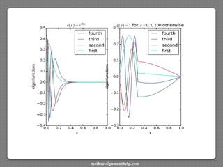
(d) For c(x) = 1, we saw in class that the eigenfunctions are sin(nπx/L). How do these
compare to the eigenvectors you plotted in the previous part? Try changing c(x) to
some other function (note: still needs to be real and > 0), and see how different you
can make the eigenfunctions from sin(nπx/L). Is there some feature that always
remains similar, no matter how much you change c?
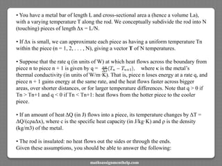
Problem 3: Discrete diffusion
In this problem, you will examine thermal conduction in a system of a finite number N
of pieces, and then take the N → ∞ limit to recover the heat equation. In particular:

• You have a metal bar of length L and cross-sectional area a (hence a volume La),
with a varying temperature T along the rod. We conceptually subdivide the rod into N
(touching) pieces of length Δx = L/N.
• If Δx is small, we can approximate each piece as having a uniform temperature Tn
within the piece (n = 1, 2, . . . , N), giving a vector T of N temperatures.
• Suppose that the rate q (in units of W) at which heat flows across the boundary from
piece n to piece n + 1 is given by q = where κ is the metal’s
thermal conductivity (in units of W/m·K). That is, piece n loses energy at a rate q, and
piece n + 1 gains energy at the same rate, and the heat flows faster across bigger
areas, over shorter distances, or for larger temperature differences. Note that q > 0 if
Tn > Tn+1 and q < 0 if Tn < Tn+1: heat flows from the hotter piece to the cooler
piece.
• If an amount of heat ΔQ (in J) flows into a piece, its temperature changes by ΔT =
ΔQ/(cρaΔx), where c is the specific heat capacity (in J/kg·K) and ρ is the density
(kg/m3) of the metal.
• The rod is insulated: no heat flows out the sides or through the ends.
Given these assumptions, you should be able to answer the following:

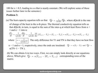
(a) “Newton’s law of cooling” says that that the temperature of an object changes at a
rate (K/s) proportional to the temperature difference with its surroundings. Derive
the equivalent here: show that our assumptions above imply that
for some constant α, for 1 < n < N. Also give the
(slightly different) equations for n = 1 and n = N.
(b) Write your equation from the previous part in matrix form:
for some matrix A.
(c) Let T (x, t) be the temperature along the rod, and suppose Tn(t) = T ([n − 0.5]Δx,
t) (the temperature at the center of the n-th piece). Take the limit N → ∞ (with L
fixed, so that and derive a partial differential equation
What is Aˆ? (Don’t worry about the x = 0, L ends until the next part.)
(d) What are the boundary conditions on T (x, t) at x = 0 and L? Check that if you go
backwards, and form a center-difference approximation of Aˆ with these boundary
conditions, that you recover the matrix A from above.
(e) How does your Aˆ change in the N → ∞ limit if the conductivity is a function
κ(x) of x?

(f) Suppose that instead of a thin metal bar (1d), you have an L × L thin metal plate
(2d), with a temperature T (x, y, t) and a constant conductivity κ. If you go through
the steps above dividing it into N × N little squares of size Δx × Δy, what PDE do you
get for T in the limit N → ∞? (Many of the steps should be similar to above.)

Problem 1
(a) We have (x, x) = x∗Bx > 0 for x = 0 by definition of positive-definiteness. We
have (x, y) = ∗ ∗ x∗By = (B∗x) y = (Bx) y = y∗(Bx) = (y, x) by B = B∗.
(b) (x, My) = x∗BMy = (M†x, y) = x∗M†∗By for all x, y, and hence we must have BM
= M†∗B ∗ , or M†∗ = BMB−1 =⇒ M† = (BMB−1) = (B−1)∗M∗B∗ . Using the fact
that
(c) If M = B−1A where A = A∗, then M† = B−1AB−1B = B−1A = M. Q.E.D.
Problem 2:
(a) As in class, let u' ([m + 0.5]Δx) ≈ u’m+0.5 = Define cm+0.5 = c([m
+ 0.5]Δx). Now we want to take the derivative of in order to
approximate Au at m by a center .5 difference:
There are other ways to solve this problem of course, that are also second-order
accurate.

(b) In order to approximate Au, we did three things: compute u' by a center-difference
as in class, multiply by cm+0.5 at each point m + 0.5, then compute the derivative by
another center-difference. The first and last steps are exactly the same center-
difference steps as in class, so they correspond as in class to multiplying by D and
−DT , respectively, where D is the (M + 1) × M matrix
The middle step, multiplying the (M + 1)-component vector u' by cm+0.5 at each
point is just multiplication by a diagonal (M + 1) × (M + 1) matrix

Putting these steps together in sequence, from right to left, means that A = −DT CD
(c) In Julia, the diagm(c) command will create a diagonal matrix from a vector c. The
function diff1(M) = [ [1.0 zeros(1,M-1)]; diagm(ones(M-1),1) - eye(M) ] will allow
you to create the (M + 1) × M matrix D from class via D = diff1(M) for any given
value of M. Using these two commands, we construct the matrix A from part (d) for
M = 100 3x and L = 1 and c(x) = e3x via
L=1
M = 100
D = diff1(M)

dx = L / (M+1)
x = dx*0.5:dx:L # sequence of x values from 0.5*dx to <= L in steps of dx
c(x) = exp(3x)
C = diagm(c(x))
A = -D’ *C*D / dx^2
You can now get the eigenvalues and eigenvectors by λ, U = eig(A), where λ is an
array of eigenvalues and U is a matrix whose columns are the corresponding
eigenvectors (notice that all the λ are < 0 since A is negative-definite).
(i) The plot is shown in Figure 1. The eigenfunctions look vaguely “sine-like”—they
have the same number of oscillations as sin(nπx/L) for n = 1, 2, 3, 4—but are
“squeezed” to the left-hand side.
(ii) We find that the dot product is ≈ 4.3 × 10−16, which is zero up to roundoff errors
(your exact value may differ, but should be of the same order of magnitude).
(iii) In the posted IJulia notebook for the solutions, we show a plot of |λ2M −λM| as a
function of M on a log–log scale, and verify that it indeed decreases ∼ 1/M2.

You can also just look at the numbers instead of plotting, and we find that this
difference decreases by a factor of ≈ 3.95 from M = 100 to M = 200 and by a factor of
≈ 3.98 from M = 200 to M = 400, almost exactly the expected factor of 4. (For fun, in
the solutions I went to M = 1600, but you only needed to go to M = 800.)
(d) In general, the eigenfunctions have the same number of nodes (sign oscillations) as
sin(nπx/L), but the oscillations pushed towards the region of high c(x). This is even
more dramatic if we increase the c(x) contrast. In Figure xxx, we show two examples.
First, c(x) = e20x, in which all of the functions are squished to the left where c is
small. Second c(x)=1 for x < 0.3 and 100 otherwise—in this case, the oscillations are
at the left 1/3 where c is small, but the function is not zero in the right 2/3. Instead, the
function is nearly constant where c is large. The reason for this has to do with the
continuity of u: it is easy to see from the operator that ' ' )' ' cu must be continuous for
(cu to exist, and hence the slope u must decrease by a factor of

Figure 2: First four eigenfunctions of Au = (cu for two different choices of c(x).

100 for x > 0.3, leading to a u that is nearly constant. (We will explore some of these
issues further later in the semester.)
Problem 3:
(a) The heat capacity equation tells us that where dQn/dt is the rate
of change of the heat in the n-th piece. The thermal conductivity equation tells us
that dQn/dt, in turn, is equal to the sum of the rates q at which heat flows from n +
1 and n − 1 into n:
where The only difference for T1 and TN is that they have no heat flow
n − 1 and n + 1, respectively, since the ends are insulated:
α(TN−1 − TN ).
(b) We can obtain A in two ways. First, we can simply look directly at our equations
above, Which give corresponding rows of the
matrix

Alternatively, we can write each of the above steps—differentiating T to get the rate of
heat flow q to the left at each of the N −1 interfaces between the pieces, then taking
the difference of the q’s to get dT /dt, in matrix form, to write:
in terms of the D matrix from class (except with N reduced by 1), which gives the
same A as above. As we will see in the parts below, this is indeed a second-derivative
approximation, but with different boundary conditions—Neumann conditions—than
the Dirichlet conditions in class.

By the way, it is interesting to consider −DDT , compared to the −DT D we had in
class. Clearly, −DDT is real-symmetric and negative semidefinite. It is not, however,
negative definite, since DT does not (and cannot) have full column rank (its rank must
be ≤ the number of rows N − 1, and in fact in class we showed that it has rank N − 1).
(c) Ignoring the ends for the moment, for all the interior points we have
which is exactly our familiar center-difference
approximation for at the point n (x = [n − 0.5]Δx). Hence,
everywhere in the interior our equations converge to and
thus
(d) The boundary conditions are The easiest way to see this is to
observe that our heat flow q is really a first derivative, and zero heat flow at the ends
Means zero derivatives. That is, qn+0.5 = is really an approximate
derivative:
qN+0.5 to/from n = 0 and n = N + 1 is zero, and hence q0.5 = qN+0.5 = 0 ≈
while the flows q0.5 and

Working backwards, consider (setting 1 for convenience)
with these boundary conditions and center-difference approximations. We are given
Tn = T([n − 0.5]Δx,t) for n = 1,...,N. First, we compute
for n = 1,...,N − 1 (−DT T using the D above). Unlike the Dirichlet case in class,
we don’t com
which are zero by the boundary conditions. Then, we compute our approximate 2nd
derivatives for n = 1,...,N, where we let
using the D from above). This gives
at the endpoints, and
for 1 <n<N,
which are precisely the rows of our A matrix above.
(e) If κ(x), then we get a different κ and α factor for each Tn+1 − Tn difference:

Where
In the N → ∞ limit, this gives
by κ, differentiated again, and then divided by cρ. (You weren’t asked to handle the
case where cρ is not a constant, so it’s okay if you commuted cρ with the derivatives.)
(f) If we discretize to Tm,n = T(mΔx, nΔy), the steps are basically the same except that
we have to consider the heat flow in both the x and y directions, and hence we have to
take differences in both x and y. In particular, suppose the thickness of the block is h. In
this case, heat will flow from Tm,n to Tm+1,n at a rate
we differentiated, multiplied
where hΔy is the area of the interface between the two blocks. Then, to convert into a
rate of temperature change, we will divide by cρhΔxΔy, where hΔxΔy is the volume of
the block. Putting this all together, we obtain:

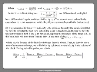
where the thing in [··· ] is precisely the five-point stencil approximation for ∇2 from
class. Hence, we obtain
where for fun I have put the κ in the middle, which is the right place if κ is not a
constant (you were not required to do this).

Online Maths Assignment Help

Recommended

Recommended

More Related Content

Similar to Online Maths Assignment Help

Similar to Online Maths Assignment Help (20)

More from Maths Assignment Help

More from Maths Assignment Help (20)

Recently uploaded

Recently uploaded (20)

Online Maths Assignment Help