The document summarizes Kepler's laws of planetary motion and provides definitions and explanations of key terms used to describe orbits of satellites around Earth. It discusses: - Kepler's 3 laws of planetary motion, including that orbits are ellipses with the primary body at one focus (1st law), areas are swept out at equal rates (2nd law), and the square of periods are proportional to cube of semi-major axes (3rd law). - Definitions of terms like apogee, perigee, inclination, and orbital elements used to characterize Earth-orbiting satellite orbits. - Factors that cause perturbations to ideal Keplerian orbits, such as Earth's oblateness, gravitational effects of

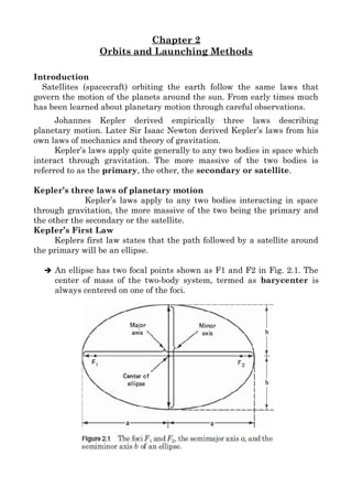
1. Chapter 2
Orbits and Launching Methods
Introduction
Satellites (spacecraft) orbiting the earth follow the same laws that
govern the motion of the planets around the sun. From early times much
has been learned about planetary motion through careful observations.
Johannes Kepler derived empirically three laws describing
planetary motion. Later Sir Isaac Newton derived Kepler’s laws from his
own laws of mechanics and theory of gravitation.
Kepler’s laws apply quite generally to any two bodies in space which
interact through gravitation. The more massive of the two bodies is
referred to as the primary, the other, the secondary or satellite.
Kepler’s three laws of planetary motion
Kepler’s laws apply to any two bodies interacting in space
through gravitation, the more massive of the two being the primary and
the other the secondary or the satellite.
KepIer’s First Law
Keplers first law states that the path followed by a satellite around
the primary will be an ellipse.
➔ An ellipse has two focal points shown as F1 and F2 in Fig. 2.1. The
center of mass of the two-body system, termed as barycenter is
always centered on one of the foci.

2. ➔ ln our specific case, because of the enormous difference between the
masses of the earth and the satellite, the center of mass coincides
with the center of the earth, which is therefore always at one of the
foci.
➔ The semimajor axis of the ellipse is denoted by a, and the semiminor
axis, by b. The eccentricity e is given by
➔ Two of the orbital parameters specified for satellites (spacecraft) orbiting
the earth are the eccentricity e and the semimajor axis, a . For an
elliptical orbit, 0 <e< 1. When e = 0, the orbit becomes circular.
P H Y S I C A L L A W S
K e p l e r ’ s 1 s t L a w : L a w o f E l l i p s e s
T h e o r b i t s o f t h e p l a n e t s a r e e l l i p s e s w i t h
t h e s u n a t o n e f o c u s
Kepler’s Second Law
Kepler’s second law states that, for equal time intervals, a satellite will
sweep out equal areas in its orbital plane, focused at the barycenter.

3. ➔ Assume the satellite travels distances S1 and S2 meters in 1 s, then
the areas A1 and A2 will be equal.
➔ The average velocity in each case is S1 and S2 m/s, and because of
the equal area law, it follows that the velocity at S2 is less than that
at S1.
➔ An important consequence of this is that the satellite takes longer to
travel a given distance when it is farther away from earth. This property
can be made use to increase the length of time a satellite can be seen from
particular geographic regions of the earth.
PHYSICAL LAWS
Kepler’s 2nd Law: Law of Equal Areas
The line joining the planet to the center of the sun
sweeps out equal areas in equal times
T6
T5
T4 T3
T2
T1A2A3A4A5
A6
A1

4. Kepler’s Third Law
Kepler’s third law states that the square of the periodic time of orbit is
proportional to the cube of the mean distance between the two bodies.
➔ The orbital period in seconds is P and the mean distance is equal to
the semimajor axis a.
P2
 a3
➔ The orbital period P is defined as the time, the orbiting body takes to
return to the same reference point in space with respect to the inertial
space.
➔ P can be written as
➔ where n is the mean motion of the satellite in radians per second.
➔ Then 
2
n

2
a3 or
➔ For the artificial satellites orbiting the earth, Kepler’s third law can be
written in the form
where n is the mean motion of the satellite in radians per second
and  is the earth’s geocentric gravitational constant or Kepler's
constant. Its value is =3.986005×1014
m3
/ s2
➔ This equation applies only to the ideal situation of a satellite orbiting a
perfectly spherical earth of uniform mass, with no perturbing forces acting,
such as atmospheric drag
➔ The importance of Kepler’s third law is that it shows there is a
fixed relationship between period and semimajor axis. One very
important orbit , known as the geostationary orbit, is determined by
the rotational period of the earth
➔ another importance of this law is that it is used to find the period of
the orbit of any satellite and is used in GPS receivers to calculate

5. positions of GPS satellite.
Explain the three features the orbit of a satellite needs to have to be perfectly
geostationary.
1. It must be exactly circular (ie e=0)
2. it must be at the correct altitude (ie have the correct period)
3. it must be in the plane of equator (ie have a zero inclination with respect
to the equator).
If the inclination is note zero and/ or if the eccentricity is not zero, but the
orbital period is correct then the satellite will be in geosynchronous orbit.
P H Y S I C A L L A W S
K e p l e r ’ s 3 r d L a w : L a w o f H a r m o n i c s
T h e s q u a r e s o f t h e p e r i o d s o f
t w o p l a n e t s ’ o r b i t s a r e
p r o p o r t i o n a l t o e a c h o t h e r a s
t h e c u b e s o f t h e i r s e m i -
m a j o r a x e s :
T 1 2 / T 2 2 = a 1 3 / a 2 3
I n E n g l i s h :
O r b i t s w i t h t h e s a m e s e m i -
m a j o r a x i s w i l l h a v e t h e
s a m e p e r i o d
Definitions of Terms for Earth-Orbiting Satellites
OR
Terms used to describe the position of the orbit with respect to
the earth.
1. Subsatellite path. This is the path traced out on the earth’s surface
directly below the satellite.

6. 2. Apogee. The point farthest from earth. Apogee height is shown as ha
in Fig. 2.3.
3. Perigee. The point of closest approach to earth. The perigee height is
shown as hp in Fig. 2.3.
ORBIT CLASSIFICATIONS
Orbit Geometry
Apogee
Perigee
cc
aEccentricity = c/a
4. Line of apsides. The line joining the perigee and apogee through the
center of the earth.

7. 5. Ascending node. The point where the orbit crosses the equatorial
plane going from south to north.
6. Descending node. The point where the orbit crosses the equatorial
plane going from north to south.
7. Line of nodes. The line joining the ascending and descending nodes
through the center of the earth.
8. Inclination. The angle between the orbital plane and the earth’s
equatorial plane. It is measured at the ascending node from the equator to
the orbit, going from east to north. The inclination is shown as i in Fig.
2.3. It will be seen that the greatest latitude, north or south, reached by
the subsatellite path is equal to the inclination.
COORDINATE SYSTEMS
Geocentric Inertial
Inclination
9. Prograde orbit. An orbit in which the satellite moves in the same
direction as the earth’s rotation, as shown in Fig. 2.4. The prograde orbit
is also known as a direct orbit. The inclination of a prograde orbit always
lies between 0° and 90°.
Most satellites are launched in a prograde orbit because the earth’s
rotational velocity provides part of the orbital velocity with a consequent
saving in launch energy.
10. Retrograde orbit. An orbit in which the satellite moves in a direction
counter to the earth’s rotation, as shown in Fig. 2.4. The inclination of a
retrograde orbit always lies between 90° and 180°

8. Argument of perigee. The angle from ascending node to perigee,
measured in the orbital plane at the earth’s center, in the direction of
satellite motion. The argument of perigee is shown as w in Fig. 2.5.

9. Right ascension of the ascending node. To define completely the
position of the orbit in space, the position of the ascending node is
specified. However, because the earth spins, while the orbital plane
remains stationary the longitude of the ascending node is not fixed, and it
cannot be used as an absolute reference. For the practical determination
of an orbit, the longitude and time of crossing of the ascending node are
frequently used. However,for an absolute measurement, a fixed reference
in space is required. The reference chosen is the first point of Aries,
otherwise known as the vernal, or spring, equinox.
The vernal equinox occurs when the sun crosses the equator going
from south to north, and an imaginary line drawn from this equatorial
crossing through the center of the sun points to the first point of Aries
(symbol ϒ). This is the line of Aries. The right ascension of the ascending
node is then the angle measured eastward, in the equatorial plane, from
the ϒ line to the ascending node, shown as Ω in Fig. 2.5.
COORDINATE SYSTEMS
Geocentric Inertial
Vernal
Equinox
Ascending Node
Direction of
Satellite motion
Right Ascension
Mean anomaly. Mean anomaly M gives an average value of the angular
position of the satellite with reference to the perigee. For a circular orbit,
M gives the angular position of the satellite in the orbit. For elliptical
orbit, the position is much more difficult to calculate.
True anomaly. The true anomaly is the angle from perigee to the
satellite position, measured at the earth’s center. This gives the true
angular position of the satellite in the orbit as a function of time.
satellite
True
anomaly

10. Orbital Elements
Earth-orbiting artificial satellites are defined by six orbital elements
referred to as the keplerian element set.
1. Semimajor axis a
2. Eccentricity e
a and e give the shape of the ellipse.
3. Mean anomaly M0, gives the position of the satellite in its orbit at a
reference time known as the epoch.
4. Argument of perigee w, gives the rotation of the orbit’s perigee point
relative to the orbit’s line of nodes in the earth’s equatorial plane. It
is shown in figure 2.5.
5. Inclination i
6. Right ascension of the ascending node Ω
i and Ω relate the orbital plane’s position to the earth.
[Note: write the definition of these terms.]
Because the equatorial bulge causes slow variations in w and Ω, and
because other perturbing forces may alter the orbital elements slightly,
the values are specified for the reference time or epoch, and thus the
epoch also must be specified.
Two-line elements
Two line elements contains a great deal of general information on
polar orbiting satellites as well as weather satellites in the geostationary
orbit.
Figure 2.6 shows how to interpret the NASA (National Aeronautics and
Space Administration) two-line elements.

12. Apogee and Perigee Heights
Although not specified as orbital elements, the apogee height and
perigee height are often required.
The length of the radius vectors at apogee and perigee can be obtained
from the geometry of the ellipse:
ra = a(1+e)
rp = a(1-e)
In order to find the apogee and perigee heights, the radius of the earth
must be subtracted from the radii lengths. ha=ra−R ; hp=rp−R
Conic section

13. SN =ZN−ZS
SN=QP−WM
SP
PQ
=e ,
SM
MW
=e
SN =
r
e
−
p
e
SN =rcos 
So ,r cos=
r
e
−
p
e
rcos −
1
e
=
−p
e
recos−1=−p
r=
p
1−ecos
r=
p
1ecosv
when=0;r=
p
1−e
=SA '
when=1800
; r=
p
1e
=SA

14. a=
AA '
2
=semimajor axis
SASA'=AA '
2a=
p
1−e

p
1e
2a=
2p
1−e2
so p=a1−e2

SA'=a
1−e2

1−e
=a1e=apogee ,ra
SA=a
1−e2

1e
=a1−e= perigee ,rp
Orbit Perturbations
The keplerian orbit is ideal in the sense that it assumes that the
earth is a uniform spherical mass and that the only force acting is the
centrifugal force resulting from satellite motion balancing the
gravitational pull of the earth.
In practice, other forces which can be significant are
a) asymmetry of earth's gravitational fields( due to nonsherical
earth)
b)the gravitational forces of the sun and the moon
c) solar radiation pressure
d) atmospheric drag.
➔ All these interfering forces cause the true orbit to be different from
Keplerian ellipse.
➔ The gravitational pulls of sun and moon have negligible effect on
low-orbiting satellites, but they do affect satellites in the
geostationary orbit.
➔ Atmospheric drag, on the other hand, has negligible effect on
geostationary satellites but does affect low orbiting earth satellites
below about 1000 km.
➔ External influences causes changes in longitude and inclination.
a) Effects of a nonspherical earth
➔ The earth is neither a perfect sphere nor a perfect ellipse.
➔ However, there being an equatorial bulge and a flattening at the
poles, a shape described as an oblate spheroid.
➔ There are regions where the average density of the earth appears to
be higher. These are called as regions of mass concentration or

15. Mascons.
➔ The nonshericity of earth , the noncircularity of the equitorial
radius, and the Mascons lead to a nonuniform gravitational field
around the earth. The force on an orbiting satellite will therefore
vary with position.
➔ For a spherical earth of uniform mass, Kepler’s third law gives the
nominal mean motion n0 as
➔ The 0 subscript is included for a perfectly spherical earth of uniform
mass.
➔ When the earth’s oblateness is taken into account, the mean motion,
denoted as n, is modified to
➔ K1 is a constant which evaluates to 66,063.1704 km2
.
➔ The earth’s oblateness has negligible effect on the semimajor axis a,
and if a is known, the mean motion is readily calculated.
➔ The orbital period taking into account the earth’s oblateness is
termed the anomalistic period (e.g., from perigee to perigee).
Because satellite does not return to the same point in space once per
revolution.
➔ The mean motion specified in the NASA bulletins is the reciprocal
of the anomalistic period.
➔ The anomalistic period is
➔ where n is in radians per second.
➔ Steps for finding a is
➔ If the known quantity is n one can solve for a, by finding the root of
the following equation:
➔ The oblateness of the earth also produces two rotations of the orbital

16. plane.
➔ 1. regression of the nodes,
2. rotation of line of apsides in the orbital plane
➔ 1. Regression of the nodes is where the nodes appear to slide along
the equator.
➔ In effect, the line of nodes, which is in the equatorial plane, rotates
about the center of the earth. Thus Ω, the right ascension of the
ascending node, shifts its position.
➔ If the orbit is prograde , the nodes slide westward, and if retrograde,
they slide eastward.
➔ As seen from the ascending node, a satellite in prograde orbit moves
eastward, and in a retrograde orbit, westward.
➔ The nodes therefore move in a direction opposite to the direction of
satellite motion, hence the term regression of the nodes.
➔ For a polar orbit (i = 90°), the regression is zero.
➔ Both effects (1 and 2) depend on the mean motion n, the semimajor
axis a, and the eccentricity e. These factors can be grouped into one
factor K given by

17. ➔ K will have the same units as n. Thus, with n in rad/day, K will be in
rad/day, and with n in degrees/day, K will be in degrees/day. An
approximate expression for the rate of change of Ω with respect to
time is
➔ where i is the inclination. The rate of regression of the nodes will
have the same units as n.
➔ When the rate of change given by the above equation is negative, the
regression is westward, and when the rate is positive, the regression
is eastward. d Ω/dt => positive => eastward
d Ω/dt => negative => westward
➔ It will be seen, therefore that for eastward regression, i must be
greater than 90o
, or the orbit must be retrograde.
Cos(0 to 90 ) is positive and cos( 90 to 180) is negative
➔ It is possible to choose values of a, e, and i such that the rate of
rotation is 0.9856°/day eastward. Such an orbit is said to be sun
synchronous
➔ 2. Rotation of line of apsides in the orbital plane,
➔ Line of apsides. The line joining the perigee and apogee through
the center of the earth.
➔ The other major effect produced by the equatorial bulge is a rotation
of the line of apsides.
➔ This line rotates in the orbital plane, resulting in the argument of
perigee changing with time. The rate of change is given by
➔ The units for the rate of rotation of the line of apsides will be the
same as those for n
➔ When the inclination i is equal to 63.435°, the term within the
parentheses is equal to zero, and hence no rotation takes place.

18. d 
dt
=k2−2.5sin
2
i
d 
dt
=0 ;
2−2.5sin
2
i=0
2.5sin
2
i=2
sin2
i=0.8 ; i=1.10714c
=
1.10714×180

=63.4349o
➔ Denoting the epoch time by t0, the right ascension of the ascending
node by Ω0, and the argument of perigee by w0 at epoch gives the new
values for Ω and w at time t as
➔ The orbit is not a physical entity, and it is the forces resulting from
an oblate earth, which act on the satellite to produce the changes in
the orbital parameters.
➔ Thus, rather than follow a closed elliptical path in a fixed plane, the
satellite drifts as a result of the regression of the nodes, and the
latitude of the point of closest approach (the perigee) changes as a
result of the rotation of the line of apsides.
➔ With this in mind, it is permissible to visualize the satellite as
following a closed elliptical orbit but with the orbit itself moving
relative to the earth as a result of the changes in Ω and w.
➔ So, The period PA is the time required to go around the orbital path
from perigee to perigee, even though the perigee has moved relative
to the earth.
➔ If the inclination is 90° ,
➔ the regression of the nodes is zero ,
➔ the rate of rotation of the line of apsides is dω/dt = −K/2

19. ➔ Imagine the situation where the perigee at the start of observations
is exactly over the ascending node. One period later the perigee
would be at an angle −KPA/2 relative to the ascending node or, in
other words, would be south of the equator.
➔
i=900
sin 90=1
d

dt
=−k×0.5
For 1sec ....
−k
2
For P A sec....
−k PA
2
➔ The time between crossings at the ascending node would be
PA (1+ K/2n), which would be the period observed from the earth.
➔ In addition to the equatorial bulge, the earth is not perfectly circular
in the equatorial plane; it has a small eccentricity of the order of
10−5.
➔ This is referred to as the equatorial ellipticity.
➔ The effect of the equatorial ellipticity is to set up a gravity gradient,
which has a pronounced effect on satellites in geostationary orbit .
➔ A satellite in geostationary orbit ideally should remain fixed
relative to the earth.
➔ The gravity gradient causes the satellites in geostationary orbit to
drift to one of two stable points, which coincide with the minor axis
of the equatorial ellipse.
➔ Due to the positions of mascons and equitorial bulges there are four
equilibrium points in the geostationary orbit.
➔ Two are stable and the other two are unstable.
➔ These two stable points are separated by 180° on the equator and
are at approximately 75° E longitude and 105° W longitude.
➔ Satellites in service are prevented from drifting to these points
through station-keeping maneuvers.
➔ Because old, out-of-service satellites eventually do drift to these
points, they are referred to as “satellite graveyards.”
➔ The effect of equatorial ellipticity is negligible on most other

20. satellite orbits.
d) Atmospheric drag
➔ For near-earth satellites, below about 1000 km, the effects of
atmospheric drag are significant.
➔ Because the drag is greatest at the perigee, the drag acts to reduce
the velocity at this point, with the result that the satellite does not
reach the same apogee height on successive revolutions.
➔ The result is that the semimajor axis and the eccentricity are both
reduced.
➔ Drag does not noticeably change the other orbital parameters,
including perigee height.
➔ In the program used for generating the orbital elements given in the
NASA bulletins, a pseudo-drag term is generated, which is equal to
one-half the rate of change of mean motion.
➔ An approximate expression for the change of major axis can be
derived as follows
➔ The change in mean motion,n is
n=n0
dn
dt
t−t0
n=n0
n'
t−t0

a0
3
=

n0
2
a3
=

n2

a
a0

3
=
n0
n

2
a=a0 
n0
n

2
3
a=a0
 n0
n0n'
t−t0
2
3
➔ where the “0” subscripts denote values at the reference time t0, and
➔ n0 ' is the first derivative of the mean motion.

21. ➔ The mean anomaly is also changed, an approximate value for the
change being:
➔ The changes resulting from the drag term will be significant only for
long time intervals, and for present purposes it will be ignored.
Inclined Orbits
➔ The orbital elements are defined with reference to the plane of the
orbit.
➔ The position of the plane of the orbit is fixed (or slowly varying) in
space.
➔ The location of the earth station is usually given in terms of the local
geographic coordinates which rotate with the earth. And the earth
station quantities may be the azimuth and elevation angles and
range.
➔ In calculations of satellite position and velocity in space, rectangular
coordinate systems are generally used .
➔ So transformations between coordinate systems are therefore
required.
➔ Calculation for elliptical inclined orbits:- the first step is to find the
earth station look angles and range
➔ The look angles for the ground station antenna are the azimuth and
elevation angles required at the antenna so that it points directly at
the satellite.
➔ Elevation is measured upward from local horizontal plane
COORDINATE SYSTEMS
Topocentric
Elevation
➔ Azimuth is measured from north eastward to the projection of the
satellite path onto the local horizontal plane

22. COORDINATE SYSTEMS
Topocentric
Azimuth
Range
Origin: Antenna
FP: Local Horizon
PD: True North
➔ Determination of the look angles and range:
The quantities used are
1. The orbital elements,
2. Various measures of time
3. The perifocal coordinate system, which is based on the orbital
plane
4. The geocentric-equatorial coordinate system, which is based on the
earth’s equatorial plane
5. The topocentric-horizon coordinate system, which is based on the
observer’s horizon plane.
➔ The satellites with inclined orbits are not geostationary, and
therefore, the required look angles and range will change with time.
➔ The two major coordinate transformations needed are:
➔ ■ The satellite position measured in the perifocal system is
transformed to the geocentric-horizon system in which the earth’s
rotation is measured, thus enabling the satellite position and the
earth station location to be coordinated.
➔ ■ The satellite-to-earth station position vector is transformed to the
topocentric-horizon system, which enables the look angles and range
to be calculated.
Calendars
➔ A calendar is a time-keeping device in which the year is divided into
months, weeks, and days.
➔ Calendar days are units of time based on the earth’s motion relative
to the sun.
➔ It is more convenient to think of the sun moving relative to the
earth.
➔ But this motion is not uniform, and so a fictitious sun, termed the
mean sun, is introduced.

23. ➔ The mean sun does move at a uniform speed but requires the same
time as the real sun to complete one orbit of the earth.
➔ Ie period of mean sun = period of real sun.
➔ This time being the tropical year.
➔ A day measured relative to this mean sun is termed a mean solar
day.
➔ Calendar days are mean solar days.
➔ A tropical year contains 365.2422 days.
➔ In order to make the calendar year, also referred to as the civil year,
it is normally divided into 365 days.
➔ The extra 0.2422 of a day is significant, and for example, after 100
years, there would be a discrepancy of 24 days between the calendar
year and the tropical year.
➔ 0.2422×100=24.22days
➔ Julius Caesar made the first attempt to correct the discrepancy by
introducing the leap year, in which an extra day is added to
February whenever the year number is divisible by 4.
➔ This gave the Julian calendar, in which the civil year was 365.25
days on average, a reasonable approximation to the tropical year.
➔ Again a difference of 0.25−0.2422 days per year exists.
➔ 0.25−0.2422×400 years=3.12days
➔ ie On every 400 years we are actually adding an extra 3 days.
➔ By the year 1582, an appreciable discrepancy once again existed
between the civil and tropical years. Pope Gregory XIII took matters
in hand by abolishing the days October 5 through October 14, 1582,
to bring the civil and tropical years into line and by placing an
additional constraint on the leap year in that years ending in two
zeros must be divisible by 400 without remainder to be reckoned as
leap years.
➔ This dodge was used to miss out 3 days every 400 years.
➔ To see this, let the year be written as X00 where X stands for the
hundreds. For example, for 1900, X = 19. For X00 to be divisible by
400, X must be divisible by 4. Now a succession of 400 years can be
written as X+ n, X+ (n+ 1), X + (n + 2), X + (n + 3),X + (n + 4),where
n is any integer from 0 to 9. If X+ n is evenly divisible by 4, then the
adjoining three numbers are not, so these three years would have to
be omitted.
➔ For example let us take X= 20 and n=0; then in the years 2000,
2100,2200, 2300, 2400, 0nly 2000 and 2400 area leap year and the
remaining are not even though it is divisible by 4.
➔ The resulting calendar is the Gregorian calendar, which is the one
in use today.

24. Universal time
➔ Universal time coordinated (UTC) is the time used for all civil time–
keeping purposes.
➔ And it is the time reference which is broadcast by the National
Bureau of Standards as a standard for setting clocks.
➔ It is based on an atomic time-frequency standard.
➔ The fundamental unit for UTC is the mean solar day.
➔ In terms of “clock time,” the mean solar day is divided into 24 h, an
hour into 60 min, and a minute into 60 s. Thus there are 86,400
“clock seconds” in a mean solar day.
➔ Satellite-orbit epoch time is given in terms of UTC.
➔ Universal time is equivalent to Greenwich mean time (GMT), as
well as Zulu (Z) time.
➔ For computations, UT will be required in two forms: as a fraction of
a day and in degrees.
➔ Given UT in the normal form of hours, minutes, and seconds, it is
converted to fractional days as
UT day
=
1
24[hours
1
60minutes
seconds
60 ] or
➔ In turn, this may be converted to degrees as
Sidereal time
➔ Sidereal time is time measured relative to the fixed stars.

25. ➔ One complete rotation of the earth relative to the fixed stars is not a
complete rotation relative to the sun.
➔ This is because the earth moves in its orbit around the sun.
➔ The sidereal day is defined as one complete rotation of the earth
relative to the fixed stars.
➔ One sidereal day has 24 sidereal hours, 1 sidereal hour has 60
sidereal minutes, and 1 sidereal minute has 60 sidereal seconds.
➔ But sidereal times and mean solar times, are different even though
both use the same basic subdivisions.
➔ The relationships between the two systems,
➔ 1 mean solar day= 1.0027379093 mean sidereal days
= 24h and (0.0027379093 x 24 )hrs
= 24 hrs 0.065709823 hrs
= 24 hrs (0. 065709823 x 60) min
= 24 hrs 3.942589392 min
= 24 hrs 3 m (0.942589392 x 60) sec
= 24 h 3 m 56.55536 s sidereal time
= 56.55536 + 3 x 60 + 24 x 60 x 60
= 86,636.55536 mean sidereal seconds
➔ 1 mean sidereal day = (1/1.0027379093 ) mean solar days
= 0.9972695664 mean solar days

26. = 23 h 56 m 04.09054 s mean solar time
= 86,164.09054 mean solar seconds
The orbital plane
or
perifocal coordinate system
➔ In the orbital plane, the position vector r and the velocity vector v
specify the motion of the satellite.
➔ Determination of position vector r : From the geometry of the ellipse
r=
p
1ecosv and p=a1−e2

➔ r can also be calculated using

27. ➔ Determination of the true anomaly , v can be done in 2 stages
Stage 1 : Find the mean anomaly M .
Stage 2 : Solve Kepler’s equation.
➔ Stage 1: The mean anomaly M at time t can be found as
➔ Here, n is the mean motion, and Tp is the time of perigee passage.
➔ For the NASA elements,
➔ Therefore,
➔ Substitute for Tp gives
➔ Stage 2 : Solve Kepler’s equation.
➔ Kepler’s equation is formulated as follows
➔ [.........

28. In satellite orbital calculations, time is often measured from the instant of
perigee passage. Denote the time of perigee passage as T and any instant
of time after perigee passage as t. Then the time interval of significance is
t - T. Let A be the area swept out in this time interval, and let Tp be the
periodic time. Then, from Kepler’s second law,
The mean motion is n = 2π/Tp and the mean anomaly is M = n (t - T).
Combining these

29. Combining

30. c= ae is the perigee, position of earth. So area is swept for the time t- T is
A
Earlier we got the area as
combining these equations
This is the Kepler’s equation....................................]
➔ Kepler’s equation is
E is the eccentric anomaly.
➔ Once E is found, v can be found from an equation known as Gauss’
equation, which is
➔ For near-circular orbits where the eccentricity is small, an
approximation for v directly in terms of M is
➔ r may be expressed in vector form in the perifocal coordinate system
(0r PQW frame) as r = (r cos v )P + (r sin v)Q

31. Local Mean Solar Time and
Sun-Synchronous Orbits
➔ The celestial sphere is an imaginary sphere of infinite radius, where
the points on the surface of the sphere represent stars or other
celestial objects.
➔ The celestial equatorial plane coincides with the earth’s equatorial
plane, and the direction of the north celestial pole coincides with the
earth’s polar axis.
➔ The the sun’s meridian is shown in figure .
➔ line of Aries is 
➔ The angular distance along the celestial equator, measured
eastward from the point of Aries to the sun’s meridian is the right
ascension of the sun, denoted by S.
➔ In general, the right ascension of a point P, is the angle, measured
eastward along the celestial equator from the point of Aries to the
meridian passing through P. This is shown as P.
➔ The hour angle of a star is the angle measured westward along the
celestial equator from the meridian to meridian of the star. Thus for

32. point P the hour angle of the sun is (P − S) measured westward
➔ In astronomy, an object's hour angle (HA) is defined as the
difference between the current local sidereal time (LST) and the
right ascension (α) of the object.
hour angle = local sidereal time (LST) - right ascension
➔ 1 HA = 15 degrees
➔ ie right ascension of the sun → S
right ascension of a point P → P
for point P the hour angle of the sun is (P − S)
➔ The apparent solar time of point P is the local hour angle of the sun,
expressed in hours, plus 12 h.
Ie apparent solar time of point P =LHA of the sun+
12 h
➔ The 12 h is added because zero hour angle corresponds to midday,
when the P meridian coincides with the sun’s meridian.
➔ Because the earth’s path around the sun is elliptical rather than
circular, and also because the plane containing the path of the
earth’s orbit around the sun (the ecliptic plane) is inclined at an
angle of approximately 23.44°, the apparent solar time does not
measure out uniform intervals along the celestial equator, in other
words, the length of a solar day depends on the position of the earth
relative to the sun.
➔ To overcome this difficulty a fictitious mean sun is introduced,
which travels in uniform circular motion around the sun.
➔ The time determined in this way is the mean solar time.

33. ➔ Figure shows the trace of a satellite orbit on the celestial sphere.
➔ Point A corresponds to the ascending node.
➔ The hour angle of the sun from the ascending node of the satellite is
Ω - S measured westward.
➔ The hour angle of the sun from the satellite (projected to S on the
celestial sphere) is Ω - S +β .
➔ thus the local mean (solar) time is
since 1 degree = 1/15 HA (hour angle)
➔ To find β:- Consider the spherical triangle defined by the points
ASB.
➔ This is a right spherical triangle because the angle between the
meridian plane through S ( projection of satellite) and the equatorial
plane is a right angle.
➔ The triangle contains the inclination i and latitude λ
➔ Inclination i is the angle between the orbital plane and the
equatorial plane.
➔ Latitude λ is the angle measured at the center of the sphere going
north along the meridian through S.
➔ The solution of the right spherical triangle gives β
tan =
SB
OB
tan i=
SB
AB
tan 
tan i
=
AB
OB
sin =
AB
OB
=sin
−1
tan
tani 
=arcsin
tan
tani 
➔ The local mean (solar) time for the satellite is therefore (by substituting the

34. value of β)
➔ As the inclination i approaches 90° angle β approaches zero.
i 90o
; tan i∞ ; 0
➔ The right ascension of the sun S can be calculated as follows,
Consider the earth completes a 360° orbit around the sun in 365.24
days.
365.24days≡3600
 ddays≡s
s=
 ddays
365.24days
×3600
➔ where Δd is the time in days from the vernal equinox (or line of
Aries  , .
➔ For a sun-synchronous orbit the local mean time must remain
constant.
➔ The advantage of a sun-synchronous orbit is that the each time the
satellite passes over a given latitude, the lighting conditions will be
approximately the same.
➔ So it can be used for placing weather satellites and environmental
satellites.
➔ Eq. for tSAT shows that for a given latitude λ and fixed inclination i ,
the only variables are S and Ω.
➔ In effect, the angle (Ω- S ) must be constant for a constant local
mean time.
➔ Let Ω0 represent the right ascension of the ascending node at the
vernal equinox and Ω' the time rate of change of Ω.

35. =0 ' t−t0
t−t0= d
➔ For this to be constant the coefficient of Δd must be zero, or
➔ The orbital elements a, e, and i can be selected to give the required
regression of 0.9856° east per day.
➔ These satellites follow near-circular, near-polar orbits.