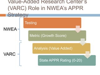
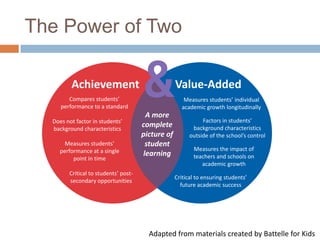
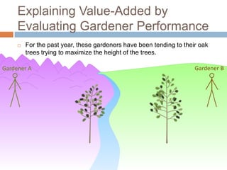
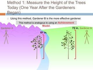
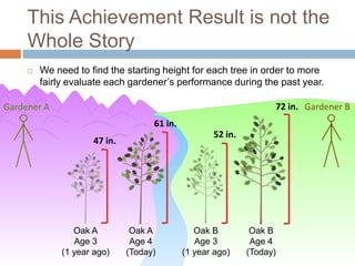
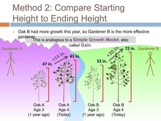
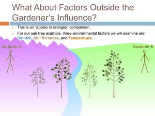
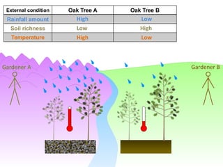
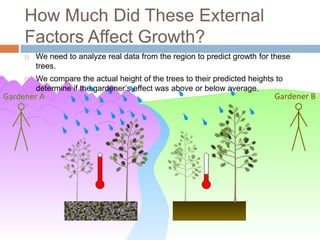
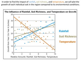
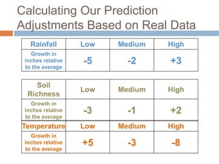
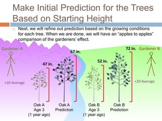
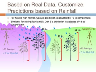
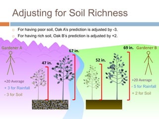
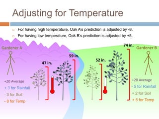
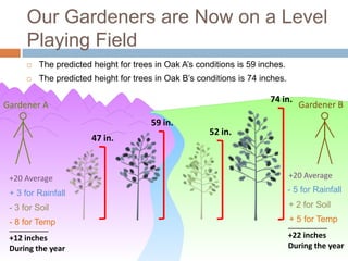
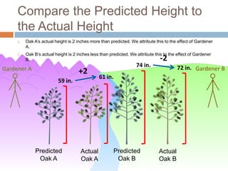
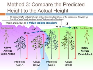
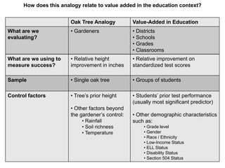
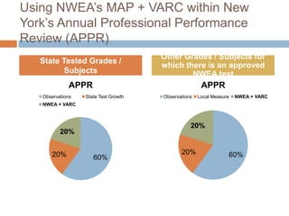
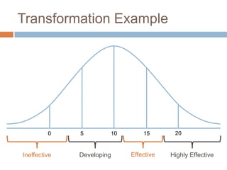
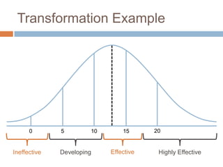
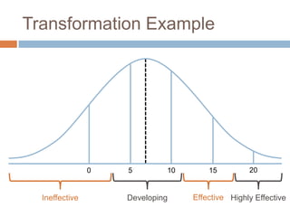
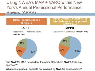
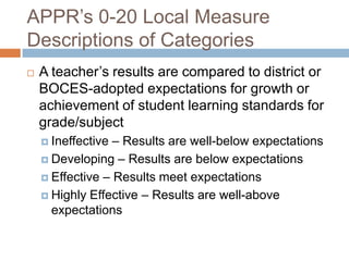
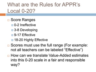
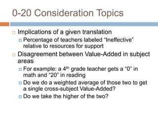
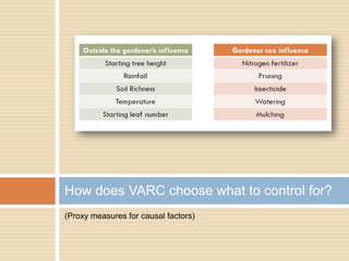
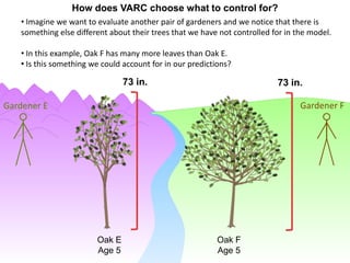
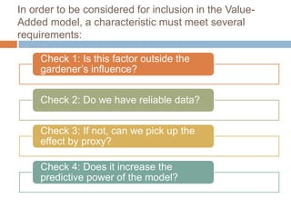
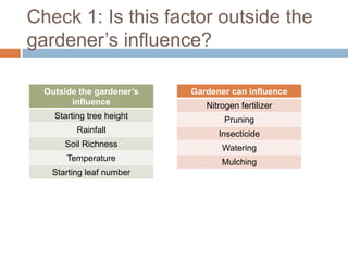
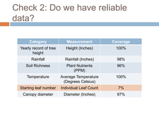
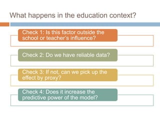
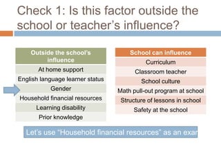
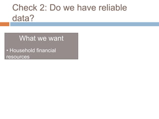
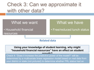
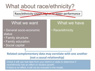
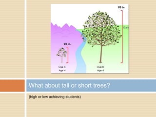
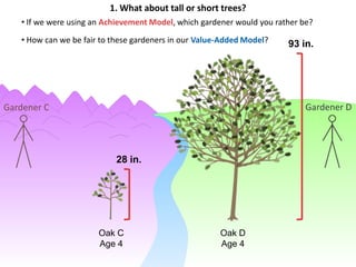
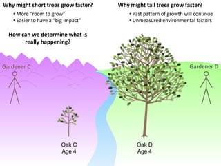
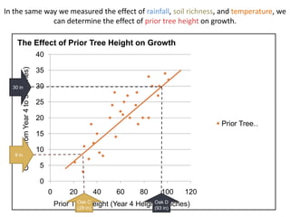
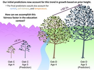
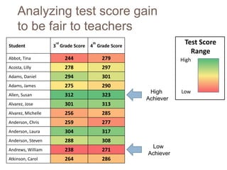
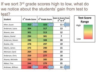
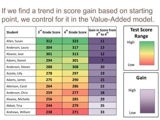
VALUE-ADDED NEW
YORK TOWN HALL
MEETING
Value-Added Research Center’s
 (VARC) Role in NWEA’s APPR
 Strategy
       Testing
NWEA
         Metric (Growth Score)


            Analysis (Value Added)
VARC
                 State APPR Rating (0-20)
The Power of Two

         Achievement
        Compares students’
     performance to a standard

  Does not factor in students’
                                       &
                                       A more
                                                   Value-Added
                                                       Measures students’ individual
                                                      academic growth longitudinally

                                                              Factors in students’
  background characteristics
                                      complete            background characteristics
                                      picture of         outside of the school’s control
      Measures students’               student
    performance at a single                               Measures the impact of
                                      learning            teachers and schools on
         point in time
                                                             academic growth
        Critical to students’ post-
                                                   Critical to ensuring students’
        secondary opportunities
                                                     future academic success


                                        Adapted from materials created by Battelle for Kids
Value-Added Basics – The Oak Tree
Analogy
The Oak Tree Analogy
Explaining Value-Added by
     Evaluating Gardener Performance
        For the past year, these gardeners have been tending to their oak
         trees trying to maximize the height of the trees.

Gardener A                                                           Gardener B
Method 1: Measure the Height of the Trees
     Today (One Year After the Gardeners
     Began)
        Using this method, Gardener B is the more effective gardener.
                This method is analogous to using an Achievement
                                      Model.
Gardener A                                                    72 in. Gardener B
                                  61 in.
Pause and Reflect
   How is this similar to how schools have been
    evaluated in the past?
   What information is missing from our gardener
    evaluation?
This Achievement Result is not the
     Whole Story
        We need to find the starting height for each tree in order to more
         fairly evaluate each gardener’s performance during the past year.

Gardener A                                                         72 in. Gardener B
                                    61 in.
                                                    52 in.
                     47 in.


                 Oak A         Oak A            Oak B         Oak B
                 Age 3         Age 4            Age 3         Age 4
              (1 year ago)    (Today)        (1 year ago)    (Today)
Method 2: Compare Starting
     Height to Ending Height
        Oak B had more growth this year, so Gardener B is the more effective
         gardener.
                This is analogous to a Simple Growth Model, also
                                    called Gain.
Gardener A                                                         72 in. Gardener B
                                    61 in.
                                                    52 in.
                     47 in.


                 Oak A         Oak A            Oak B         Oak B
                 Age 3         Age 4            Age 3         Age 4
              (1 year ago)    (Today)        (1 year ago)    (Today)
What About Factors Outside the
     Gardener’s Influence?
        This is an “apples to oranges” comparison.
        For our oak tree example, three environmental factors we will examine are:
         Rainfall, Soil Richness, and Temperature.

Gardener A                                                                 Gardener B
External condition   Oak Tree A   Oak Tree B
 Rainfall amount        High          Low
  Soil richness         Low           High
   Temperature          High          Low


Gardener A                                      Gardener B
How Much Did These External
     Factors Affect Growth?
        We need to analyze real data from the region to predict growth for these
         trees.
        We compare the actual height of the trees to their predicted heights to
         determine if the gardener’s effect was above or below average.
Gardener A                                                                   Gardener B
In order to find the impact of rainfall, soil richness, and temperature, we will plot the
growth of each individual oak in the region compared to its environmental conditions.
Calculating Our Prediction
Adjustments Based on Real Data
   Rainfall        Low   Medium   High
   Growth in
 inches relative   -5      -2     +3
 to the average


     Soil
                   Low   Medium   High
  Richness
   Growth in
 inches relative   -3      -1     +2
 to the average
Temperature        Low   Medium   High
   Growth in
 inches relative   +5      -3     -8
 to the average
Make Initial Prediction for the Trees
     Based on Starting Height
        Next, we will refine out prediction based on the growing conditions
         for each tree. When we are done, we will have an “apples to apples”
         comparison of the gardeners’ effect.

Gardener A                                                              72 in. Gardener B
                                       67 in.

                                                       52 in.
                      47 in.


 +20 Average                                                                 +20 Average


                  Oak A          Oak A             Oak B         Oak B
                  Age 3        Prediction          Age 3        Prediction
               (1 year ago)                     (1 year ago)
Based on Real Data, Customize
     Predictions based on Rainfall
        For having high rainfall, Oak A’s prediction is adjusted by +3 to compensate.
        Similarly, for having low rainfall, Oak B’s prediction is adjusted by -5 to
         compensate.
Gardener A                              70 in.                           67 in. Gardener B

                                                        52 in.
                       47 in.


 +20 Average                                                                  +20 Average

 + 3 for Rainfall                                                             - 5 for Rainfall
Adjusting for Soil Richness
         For having poor soil, Oak A’s prediction is adjusted by -3.
         For having rich soil, Oak B’s prediction is adjusted by +2.


Gardener A                                                              69 in. Gardener B
                                        67 in.

                                                        52 in.
                        47 in.


 +20 Average                                                                +20 Average

 + 3 for Rainfall                                                           - 5 for Rainfall

 - 3 for Soil                                                               + 2 for Soil
Adjusting for Temperature
         For having high temperature, Oak A’s prediction is adjusted by -8.
         For having low temperature, Oak B’s prediction is adjusted by +5.

                                                                      74 in.
Gardener A                                                                     Gardener B
                                       59 in.
                                                      52 in.
                       47 in.


 +20 Average                                                               +20 Average

 + 3 for Rainfall                                                          - 5 for Rainfall

 - 3 for Soil                                                              + 2 for Soil
 - 8 for Temp                                                              + 5 for Temp
Our Gardeners are Now on a Level
      Playing Field
         The predicted height for trees in Oak A’s conditions is 59 inches.
         The predicted height for trees in Oak B’s conditions is 74 inches.

                                                                       74 in.
Gardener A                                                                        Gardener B
                                        59 in.
                                                       52 in.
                        47 in.


 +20 Average                                                                   +20 Average

 + 3 for Rainfall                                                              - 5 for Rainfall

 - 3 for Soil                                                                  + 2 for Soil
 - 8 for Temp                                                                  + 5 for Temp
 _________                                                                     _________
 +12 inches                                                                    +22 inches
 During the year                                                               During the year
Compare the Predicted Height to
     the Actual Height
        Oak A’s actual height is 2 inches more than predicted. We attribute this to the effect of Gardener
         A.
        Oak B’s actual height is 2 inches less than predicted. We attribute this to the effect of Gardener
         B.                                                                     -2
                                                                   74 in.                72 in. Gardener B
Gardener A                           +2
                                               61 in.
                          59 in.


              Predicted               Actual           Predicted               Actual
               Oak A                  Oak A             Oak B                  Oak B
Method 3: Compare the Predicted
     Height to the Actual Height
        By accounting for last year’s height and environmental conditions of the trees during this year, we
         found the “value” each gardener “added” to the growth of the trees.

    This is analogous to a Value-Added measure.                                -2
                                             74 in.                                     72 in. Gardener B
Gardener A                   +2
                                   61 in.
                      59 in.


   Above                                                                                          Below
  Average                                                                                        Average
Value-Added                                                                                    Value-Added

              Predicted              Actual           Predicted               Actual
               Oak A                 Oak A             Oak B                  Oak B
Value-Added Basics – Linking the Oak Tree
Analogy to Education
How does this analogy relate to value added in the education context?


                        Oak Tree Analogy          Value-Added in Education
What are we             • Gardeners               • Districts
evaluating?                                       • Schools
                                                  • Grades
                                                  • Classrooms
What are we using to    • Relative height         • Relative improvement on
measure success?        improvement in inches     standardized test scores

Sample                  • Single oak tree         • Groups of students

Control factors         • Tree’s prior height     • Students’ prior test performance
                                                  (usually most significant predictor)
                        • Other factors beyond
                        the gardener’s control:   • Other demographic characteristics
                             • Rainfall           such as:
                             • Soil richness           • Grade level
                             • Temperature             • Gender
                                                       • Race / Ethnicity
                                                       • Low-Income Status
                                                       • ELL Status
                                                       • Disability Status
                                                       • Section 504 Status
Another Visual Representation
 The Education Context                          Actual student
                                                 achievement
                                                  RIT score


                                                          Value-
  Starting
  student                                                 Added
achievement
 RIT score
                              Predicted student
                                achievement
                          (Based on observationally
                              similar students)


              Fall NWEA           Spring NWEA
              MAP Score            MAP Score
VARC Data Output
What do Value-Added Results Look
Like?
   The Value-Added model typically generates a
    set of results measured in scale scores.
                                 This teacher’s students
                                gained 10 more points on
                 Value-             the RIT scale than
    Teacher                       observationally similar
                 Added          students across the state.
                                   (10 points more than
Teacher A          +10                  predicted)
                                  10 points fewer than
                                       predicted
Teacher B          -10
                                 These students gained
                                exactly as many points as
Teacher C           0                    predicted
Value-Added in “Tier” Units

                              -2   -1   0    1    2


In some cases, Value-
Added is displayed on
“Tier” scale based on
                                            0.9
 Grade 4
standard deviations (z-30
score) for reporting
purposes.

About 95% of estimates
will fall between -2 and +2
on the scale.
Using NWEA’s MAP + VARC within New
York’s Annual Professional Performance
Review (APPR)
                                      Other Grades / Subjects for
   State Tested Grades /
                                      which there is an approved
         Subjects                             NWEA test
             APPR                                     APPR
   Observations   State Test Growth   Observations   Local Measure   NWEA + VARC
   NWEA + VARC


                                                 20%
          20%


      20%                                    20%                 60%
                     60%
APPR’s 0-20 Local Measure
Descriptions of Categories
   A teacher’s results are compared to district or
    BOCES-adopted expectations for growth or
    achievement of student learning standards for
    grade/subject
     Ineffective – Results are well-below expectations
     Developing – Results are below expectations

     Effective – Results meet expectations

     Highly Effective – Results are well-above
      expectations
What are the Rules for APPR’s
Local 0-20?
   Score Ranges
     0-2 Ineffective
     3-8 Developing

     9-17 Effective

     18-20 Highly Effective
What are the Rules for APPR’s
Local 0-20?
   Scores must use the full range (For example:
    not all teachers can be labeled “Effective”)
   How can we translate Value-Added estimates
    into this 0-20 scale in a fair and responsible
    way?
     Who gets labeled “Ineffective”
     Resources to support these teachers
Transformation Example


         0    5        10       15       20


Ineffective   Developing    Effective   Highly Effective
Transformation Example


      0       5        10       15      20


Ineffective   Developing    Effective    Highly Effective
Transformation Example


         0    5        10       15       20


Ineffective   Developing    Effective   Highly Effective
Transformation Example


                0   5        10       15         20


  Ineffective       Developing    Effective Highly Effective
VARC Data Output File
Example VARC Output File
                 What is included in
                  these results?
Levels of Results
    District     School      Teacher     Grade   Subject
    District A   School 1   Ms. Smith      4      Math
    District A   School 1   Ms. Smith      4     Reading
    District A   School 2   Mr. Jones      6      Math
                                                 Language
    District A   School 3   Mr. Thomas     1
                                                  Usage
    District A   School 4   Mrs. Meyer    10     Reading

   Results will be provided for (provided a large
    enough sample of students)
      Math grades K-10

      Reading grades K-10

      Language Usage grades K-10
Result Formats

               Confidence                     Confidence          0-20
RIT Score                         Tier
                Interval                       Interval          APPR
   +10          +7 to +13         +1.9        +1.7 to +2.1         18
    0            -2 to +2           0          -0.2 to +0.2        10
    -4           -6 to -2         -0.8         -1.0 to -0.6         7


     Scale score growth        “z-scores” of the RIT score     Default 0-20
difference than average for   differences. This answers the   to comply with
   observationally similar             question of               law (to be
          students                 “how good is good?”            decided)
VARC Data Needs
What Data Does VARC Need?
   Data identifying and linking students/teachers
     StateStudent ID linkable to NWEA data
     School ID

     Teacher ID
What Data Does VARC Need?
   Student Test Data
     FallTest Data for Math, Reading, Language
      Usage
      (Date, Score, SEM)
     Spring Test Data for Math, Reading, Language
      Usage
      (Date, Score)
   Student Demographics
     Grade,  Gender, Race/Ethnicity, Special Education
      Status, ELL Status, FRL Status, etc.
What is the Timeline?
   Testing windows in the 2012-2013 school year
     Need   Fall/Spring testing
   Collection strategy for student demographic
    data
     Data from the state update
     Contingency plan for collection from RIC/district
What is the Timeline?
   Our production timeline can only begin once
    we’ve received clean student-teacher linking
    data from supplier (state, RIC, district)
   Timeline for Value-Added analysis
     Drop-dead  date for data transfer to VARC
     Time to run analysis and quality check

     Return results back to districts’ superintendants or
      designee
   Special case of summer 2012
Questions / concerns for the
advisory committee to address?
•   Individual student-level MAP growth targets
    vs. the need for Value-Added for APPR
•   0-20 local measure within APPR 0-100
•   Transformation of Value-Added to 0-20
•   Consistent messaging and meaning across
    NWEA partners
•   Approving this solution through the New
    York SED
VALUE-ADDED NEW
YORK ADVISORY GROUP
MEETING
Existing VARC Projects
Districts and States Working with
 VARC

               NORTH DAKOTA   MINNESOTA

                    Minneapolis      WISCONSIN
               SOUTH DAKOTA                      Milwaukee
                                Madison               Racine

                                                     Chicago             New York City
                                          ILLINOIS
              Denver


                                 Tulsa
                                                               Atlanta
Los Angeles


                                                                         Hillsborough County

                                                     Collier County
Wisconsin
               Opt-in statewide Value-
                Added system (2010)
               Statewide advisory group
                with quarterly meetings
                 District-led annual meetings
                  on responsible use and
                  messaging
                 Expansion of piloted MAP
                  Value-Added (Racine and
                  Milwaukee) to statewide
                  model
               Same model and
                messaging across districts
A Value-Added Model of Classroom
     Performance: Recipe for a Statistician


                 Y1i    Y0i    X i 
  
k (school)
             1k S1ik                  
                          k (school) j (classroom)
                                                     1 jk C1ijk  1i
What does that mean in
  English?
                                                                                 Error term for
                                               Adjustment to
                  Adjustment to                                                 unknown factors,
                                                account for
                   account for                                                   (reduces with
                                                  student
                  starting point                                               increased sample
                                               demographics
                                                                                     size)


                                                                                       Unknown
                                                 Student
                Post-on-                                            Classroo            Student
Post-Test   =   Pre Link   *    Pre-Test   +   Characteristi
                                                   cs
                                                               +    m Effect    +     Characteristi
                                                                                          cs


                                                                      Classroom
  Spring MAP                                                        contribution to
                               Fall MAP Result                     student learning
    Result
                                                                    (Value-Added)
Los Angeles, California

                 Phase 1 (May 2011)
                   Grades 3-8 Math and ELA
                   Grade 9 ELA

                 Phase 2 (Nov 2011)
                   Grades 3-11 ELA
                   Grades 3-8 General Math
                   High School subjects
                         Math, ELA, Science, Social
                          Studies
                 Phase 3 (Nov 2012)
                     Other Assessments
Example Documentation
                                    Excerpt from LAUSD’s
                                     teacher-level Value-
                                         Added Model
                                        documentation

                                     Transparency of the
                                      model is our goal


   http://portal.battelleforkids.org/BFK/LAUSD/Tra
    ining_Materials.html?sflang=en
Hillsborough County, Florida

   Began July 2010
   Subject / Grade Coverage
       Models from Art to Welding
   Multiple Measures
       Charlotte Danielson observational
        ratings
       Combined use of student
        outcomes and observational data
        in evaluation system
   Use of Value-Added
       Fiscal awards
       Future uses being developed
        together with union
New York, New York
                 In the past, Value-
                  Added based on state
                  exams
                   Dangers related to the
                    release of teacher-level
                    data
                   Constructive use of data

                 Currently calculating
                  local measures based
                  on MAP
                 Advising NYC on
                     Transformation to 0-20
Some Common Features of
VARC’s Value-Added Models
   Prior test scores to predict current test scores
       Single prior test or multiple tests (sometimes across
        subjects)
       Growth of a teacher’s students is compared to growth of
        similarly achieving students across the state
   Student demographics
       Typically Gender, Race/Ethnicity, Low-Income
        Status, Special Education Status, English Language
        Learner Status, other student-level data available for all
        students
   Measurement error correction
   Dosage (when enrollment data is available)
   Statistical shrinkage estimation
   VARC motto: Simpler is better unless it’s wrong
       Continuous improvement of the model based on latest
        research and improving data quality
Translating Value-Added to the 0-20
Scale Required by APPR
Using NWEA’s MAP + VARC within New
York’s Annual Professional Performance
Review (APPR)
                                         Other Grades / Subjects for
      State Tested Grades /
                                         which there is an approved
            Subjects                             NWEA test
                APPR                                     APPR
      Observations   State Test Growth   Observations   Local Measure   NWEA + VARC
      NWEA + VARC


                                                    20%
             20%


         20%                                    20%                 60%
                        60%


Can NWEA’s MAP be used for the other 20% where NWEA tests are
approved?
What about grades / subjects not covered by NWEA’s assessments?
APPR’s 0-20 Local Measure
Descriptions of Categories
   A teacher’s results are compared to district or
    BOCES-adopted expectations for growth or
    achievement of student learning standards for
    grade/subject
     Ineffective – Results are well-below expectations
     Developing – Results are below expectations

     Effective – Results meet expectations

     Highly Effective – Results are well-above
      expectations
What are the Rules for APPR’s
Local 0-20?
   Score Ranges
     0-2 Ineffective
     3-8 Developing

     9-17 Effective

     18-20 Highly Effective

   Scores must use the full range (For example:
    not all teachers can be labeled “Effective”)
   How can we translate Value-Added estimates
    into this 0-20 scale in a fair and responsible
    way?
Transformation Example


         0    5        10       15       20


Ineffective   Developing    Effective   Highly Effective
Transformation Example


      0       5        10       15      20


Ineffective   Developing    Effective    Highly Effective
Transformation Example


         0    5        10       15       20


Ineffective   Developing    Effective   Highly Effective
Transformation Example


                0   5        10       15         20


  Ineffective       Developing    Effective Highly Effective
0-20 Consideration Topics
   Implications of a given translation
     Percentage    of teachers labeled “Ineffective”
      relative to resources for support
   Disagreement between Value-Added in subject
    areas
     For example: a 4th grade teacher gets a “0” in
      math and “20” in reading
     Do we do a weighted average of those two to get
      a single cross-subject Value-Added?
     Do we take the higher of the two?
0-20 Consideration Topics
   What about teachers teaching multiple
    grades?
     Same     solution as multi-subject?
   Once multiple years of data are available, do
    we use the most recent year or a multi-year
    average?
     If   an average, how many years?
   What about estimates based on very few
    students?
     Is there a minimum threshold for reporting out?
     Is there any way to consider the confidence
Break
15 Minutes
Modeling Decisions
Why does VARC recommend including
student demographic data?
How do we decide what to include?
How does VARC choose what to control for?
(Proxy measures for causal factors)
How does VARC choose what to control for?
   • Imagine we want to evaluate another pair of gardeners and we notice that there is
   something else different about their trees that we have not controlled for in the model.

   • In this example, Oak F has many more leaves than Oak E.
   • Is this something we could account for in our predictions?

                                73 in.                                     73 in.

Gardener E                                                                        Gardener F


                        Oak E                             Oak F
                        Age 5                             Age 5
In order to be considered for inclusion in the Value-
Added model, a characteristic must meet several
requirements:

     Check 1: Is this factor outside the
     gardener’s influence?


     Check 2: Do we have reliable data?


     Check 3: If not, can we pick up the
     effect by proxy?

     Check 4: Does it increase the
     predictive power of the model?
Check 1: Is this factor outside the
gardener’s influence?

  Outside the gardener’s   Gardener can influence
        influence             Nitrogen fertilizer
    Starting tree height           Pruning
          Rainfall               Insecticide
      Soil Richness               Watering
       Temperature                Mulching
   Starting leaf number
Check 2: Do we have reliable
data?

      Category              Measurement          Coverage
 Yearly record of tree     Height (Inches)        100%
        height
       Rainfall            Rainfall (Inches)       98%
    Soil Richness           Plant Nutrients        96%
                                (PPM)
    Temperature          Average Temperature      100%
                          (Degrees Celsius)
 Starting leaf number    Individual Leaf Count     7%
  Canopy diameter         Diameter (Inches)        97%
Check 3: Can we approximate it
with other data?

         Category              Measurement          Coverage
    Yearly record of tree     Height (Inches)        100%
           height
          Rainfall            Rainfall (Inches)       98%
       Soil Richness           Plant Nutrients        96%
                                   (PPM)
       Temperature          Average Temperature      100%
                             (Degrees Celsius)

?   Starting leaf number    Individual Leaf Count     7%
     Canopy diameter         Diameter (Inches)        97%
Canopy diameter as a proxy for leaf count
   • The data we do have available about canopy diameter might help us measure the effect
   of leaf number.
   • The canopy diameter might also be picking up other factors that may influence tree
   growth.
   • We will check its relationship to growth to determine if it is a candidate for inclusion in
   the model.


Gardener E                                                                           Gardener F


                    33 in.                          55 in.


                         Oak E                               Oak F
                         Age 5                               Age 5
If we find a relationship between starting tree diameter and growth, we would
        want to control for starting diameter in the Value-Added model.

The Effect of Tree Diameter on Growth
                                     40
  Growth from Year 5 to 6 (inches)


                                     35

                                     30

                                     25

                                     20
                                                               ?                             Tree Diameter
                                     15

                                     10

                                     5

                                     0
                                          0           20         40        60           80
                                              Tree Diameter (Year 5 Diameter in Inches)
If we find a relationship between starting tree diameter and growth, we would
        want to control for starting diameter in the Value-Added model.

The Effect of Tree Diameter on Growth
                                     40
  Growth from Year 5 to 6 (inches)


                                     35

                                     30

                                     25

                                     20
                                                                                             Tree Diameter
                                     15

                                     10

                                     5

                                     0
                                          0           20         40        60           80
                                              Tree Diameter (Year 5 Diameter in Inches)
What happens in the education context?

   Check 1: Is this factor outside the
   school or teacher’s influence?


   Check 2: Do we have reliable data?


   Check 3: If not, can we pick up the
   effect by proxy?

   Check 4: Does it increase the
   predictive power of the model?
Check 1: Is this factor outside the
school or teacher’s influence?

    Outside the school’s              School can influence
         influence                          Curriculum
       At home support                  Classroom teacher
English language learner status           School culture
           Gender                 Math pull-out program at school
Household financial resources      Structure of lessons in school
      Learning disability              Safety at the school
       Prior knowledge

   Let’s use “Household financial resources” as an example
Check 2: Do we have reliable
  data?

     What we want
• Household financial
resources
Check 3: Can we approximate it
  with other data?

     What we want                               What we have
• Household financial                      • Free/reduced lunch status
resources

                                Related data

       Using your knowledge of student learning, why might
     “household financial resources” have an effect on student
                             growth?
 Check 4: “Does it increase the predictive power of the model?” will be
 determined by a multivariate linear regression model based on real data from
 your district or state (not pictured) to determine whether FRL status had an
 effect on student growth.
What about race/ethnicity?
         Race/ethnicity causes higher or lower performance


      What we want                                  What we have
• General socio-economic            • Race/ethnicity
status
• Family structure
• Family education
• Social capital
• Environmental stress
   Related complementary data may correlate with one another
                   (not a causal relationship)
 Check 4 will use real data from your district or state to determine if
 race/ethnicity has an effect on student growth.
 If there is no effect, it will not be included in the model.
What about race/ethnicity?
If there is a detectable difference in growth rates

   We attribute this to a district or state
    challenge to be addressed
   Not as something an individual teacher or
    school should be expected to overcome on
    their own
Checking for Understanding
   What would you tell a 5th grade teacher who
    said they wanted to include the following in the
    Value-Added model for their results?:
    A.   5th grade reading curriculum
    B.   Their students’ attendance during 5th grade
    C.   Their students’ prior attendance during 4th grade
    D.   Student motivation
              Check 1: Is this factor outside the school or teacher’s
              influence?


              Check 2: Do we have reliable data?


              Check 3: If not, can we pick up the effect by proxy?


              Check 4: Does it increase the predictive power of the model?
Small Group Discussion

Group 1          Key discussion topics:
Nate (NWEA)        Advisory  council’s role in selecting a
Sean (VARC)         consistent “standard” model and 0-
                    20 translation and Value-Added
                    model
Group 2
                   Questions / concerns about
John (NWEA)         selecting a 0-20 translation of Value-
Andrew              Added
(VARC)
                   Questions / concerns about
                    modeling features (we do not yet
                    know what data will be available to
                    VARC)
Wrap-Up
   Top concerns and questions from small group
    discussion
   Where do we need more information?
   What are the challenges we face?
     How can we work together to address those
     challenges?
   What are our next steps?
     Nextadvisory group meeting
     What topics should we cover?
Additional Resources
Quasi-experimental design structure
Visualizing Achievement vs. Value-Added
Controlling for starting point
Comparison to a different model – Student Growth
Percentiles
Value-Added Model Description


Design                              Output                                Objective
• Quasi-experimental statistical    • Productivity estimates for          • Valid and fair comparisons of
  model                               contribution of educational units     school productivity, given that
• Controls for non-school factors     (schools, classrooms, teachers)       schools may serve very different
  (prior achievement, student and     to student achievement growth         student populations
  family characteristics)
The Power of Two - Revisited
                          100
                                                                                Scatter plots are a way to
                                                                                represent Achievement and
Percent Prof/Adv (2009)


                          80                                                    Value-Added together
                                    Achievement


                          60


                          40


                          20

                                                        Value-Added
                           0
                                1                  2        3         4     5
                                                  Value-Added (2009-2010)
The Power of Two - Revisited
                                                                  A. Students know a lot and are
                          100                                     growing faster than predicted
                                    C                     A       B. Students are behind, but are
Percent Prof/Adv (2009)


                          80                                      growing faster than predicted

                                              E                   C. Students know a lot, but are
                          60                                      growing slower than predicted

                                                                  D. Students are behind, and
                          40                                      are growing slower than
                                                          B       predicted
                                     D                            E. Students are about average
                          20                                      in how much they know and
                                                                  how fast they are growing
                           0
                                1       2     3       4       5
                                                                           Schools in your district
                                    Value-Added (2009-2010)
What about tall or short trees?
(high or low achieving students)
1. What about tall or short trees?
   • If we were using an Achievement Model, which gardener would you rather be?

   • How can we be fair to these gardeners in our Value-Added Model?    93 in.


Gardener C                                                                   Gardener D


                           28 in.


                       Oak C                           Oak D
                       Age 4                           Age 4
Why might short trees grow faster?   Why might tall trees grow faster?
   • More “room to grow”                 • Past pattern of growth will continue
   • Easier to have a “big impact”       • Unmeasured environmental factors

  How can we determine what is
       really happening?


Gardener C                                                          Gardener D


                        Oak C               Oak D
                        Age 4               Age 4
In the same way we measured the effect of rainfall, soil richness, and temperature, we
              can determine the effect of prior tree height on growth.

    The Effect of Prior Tree Height on Growth
                                             40
          Growth from Year 4 to 5 (inches)


                                             35

  30 in                                      30

                                             25

                                             20
                                                                                                       Prior Tree…
                                             15

                                             10
   9 in

                                             5

                                             0
                                                  0        20      40     60      80     100     120
                                                              Oak C                   Oak D
                                                      Prior Treein)
                                                              (28
                                                                  Height (Year 4 Height inin)
                                                                                      (93
                                                                                            Inches)
Our initial predictions now account for this trend in growth based on prior height.
  • The final predictions would also account for
      rainfall, soil richness, and temperature.

  How can we accomplish this
fairness factor in the education
            context?


    Oak C         Oak C                            Oak D                Oak D
    Age 4          Age 5                           Age 4                 Age 5
                (Prediction)                                          (Prediction)
Analyzing test score gain
     to be fair to teachers
Student
                     rd
                    3 Grade Score
                                     th
                                    4 Grade Score
                                                                Test Score
                                                                  Range
Abbot, Tina               244             279                  High
Acosta, Lilly             278             297
Adams, Daniel             294             301
Adams, James              275             290
                                                     High      Low
Allen, Susan              312             323
                                                    Achiever
Alvarez, Jose             301             313
Alvarez, Michelle         256             285
Anderson, Chris           259             277
Anderson, Laura           304             317
Anderson, Steven          288             308
                                                     Low
Andrews, William          238             271
                                                    Achiever
Atkinson, Carol           264             286
If we sort 3rd grade scores high to low, what do
we notice about the students’ gain from test to
test?
 Student
                      rd
                     3 Grade Score
                                      th
                                     4 Grade Score
                                                     Gain in Score from
                                                           rd    th
                                                                           Test Score
                                                          3 to 4
                                                                             Range
 Allen, Susan              312             323              11            High
 Anderson, Laura           304             317              13
 Alvarez, Jose             301             313              12
 Adams, Daniel             294             301               7
                                                                          Low
 Anderson, Steven          288             308              20
 Acosta, Lilly             278             297              19
 Adams, James              275             290              15
 Atkinson, Carol           264             286              22
 Anderson, Chris           259             277              18
 Alvarez, Michelle         256             285              29
 Abbot, Tina               244             279              35
 Andrews, William          238             271              33
If we find a trend in score gain based on starting
point, we control for it in the Value-Added model.
 Student
                      rd
                     3 Grade Score
                                      th
                                     4 Grade Score
                                                     Gain in Score from
                                                           rd    th
                                                                           Test Score
                                                          3 to 4
                                                                             Range
 Allen, Susan              312             323              11            High
 Anderson, Laura           304             317              13
 Alvarez, Jose             301             313              12
 Adams, Daniel             294             301               7
                                                                          Low
 Anderson, Steven          288             308              20
 Acosta, Lilly             278             297              19
 Adams, James              275             290              15                   Gain
 Atkinson, Carol           264             286              22
                                                                          High
 Anderson, Chris           259             277              18
 Alvarez, Michelle         256             285              29
 Abbot, Tina               244             279              35
 Andrews, William          238             271              33             Low
What do we usually find in
reality?
   Looking purely at a simple growth model, high
    achieving students tend to gain about 10%
    fewer points on the test than low achieving
    students.
   In a Value-Added model we can take this into
    account in our predictions for your students, so
    their growth will be compared to similarly
    achieving students.
Comparisons of gain at different schools
  before controlling for prior performance


   School A        School B         School C     Student
                                                Population
                                               Advanced
                                               Proficient
                                               Basic
                                               Minimal
    High           Medium          Low
Achievement      Achievement   Achievement     Why isn’t
  Artificially                 Artificially    this fair?
 lower gain                     inflated
Comparisons of Value-Added at different
                 schools
 after controlling for prior performance


School A    School B    School C    Student
                                   Population
                                   Advanced
                                   Proficient
                                   Basic
                                   Minimal

Fair        Fair        Fair
Checking for Understanding
   What would you tell a teacher or principal who
    said Value-Added was not fair to schools with:
     Highachieving students?
     Low achieving students?

   Is Value-Added incompatible with the notion of
    high expectations for all students?
STUDENT GROWTH
  PERCENTILES (SGP)

Draft Explanation
How Would SGP Measure Oak
     A?
        Oak A’s growth will be compared to all Oaks in the region who
         started at the same height last year.

Gardener A


                     47 in.


                Oak A          Oak A
                Age 3          Age 4
             (1 year ago)     (Today)
Identify all Oaks that were 47” last
   year


   Oak A     Oak T   Oak U   Oak V   Oak W   Oak X   Oak Y   Oak Z
   Age 3
(1 year ago)
Find the Height of Those Trees
 Today


 Oak A    Oak T   Oak U   Oak V   Oak W   Oak X   Oak Y   Oak Z
 Age 4
(Today)
Reorder the Trees Shortest to
 Tallest


 Oak A    Oak T   Oak U   Oak V   Oak W   Oak X   Oak Y   Oak Z
 Age 4
(Today)
Reorder the Trees Shortest to
Tallest
   The percentage of trees equal or shorter than
    Oak A is Oak A’s growth percentile.


Oak W      Oak A    Oak U     Oak T    Oak Z   Oak Y   Oak X   Oak V
           Age 4
          (Today)

    2/8 = 0.25      25th Growth Percentile
Assigning SGP to the Gardener
        If Gardener A is assigned to multiple trees, the median SGP of
         Gardener A’s trees is assigned to the Gardener.

Gardener A
                                    61 in.
                     47 in.


  25th
Percentile


                 Oak A         Oak A
                 Age 3         Age 4
              (1 year ago)    (Today)
Pause and Reflect
   What might happen if Oak A is in a different
    environment than the other trees it was
    compared against?
   Is SGP measuring the effect of just the
    gardener?

New York Town Hall Value Added - VARC

  • 1.
  • 2.
    Value-Added Research Center’s (VARC) Role in NWEA’s APPR Strategy Testing NWEA Metric (Growth Score) Analysis (Value Added) VARC State APPR Rating (0-20)
  • 3.
    The Power ofTwo Achievement Compares students’ performance to a standard Does not factor in students’ & A more Value-Added Measures students’ individual academic growth longitudinally Factors in students’ background characteristics complete background characteristics picture of outside of the school’s control Measures students’ student performance at a single Measures the impact of learning teachers and schools on point in time academic growth Critical to students’ post- Critical to ensuring students’ secondary opportunities future academic success Adapted from materials created by Battelle for Kids
  • 4.
    Value-Added Basics –The Oak Tree Analogy
  • 5.
    The Oak TreeAnalogy
  • 6.
    Explaining Value-Added by Evaluating Gardener Performance  For the past year, these gardeners have been tending to their oak trees trying to maximize the height of the trees. Gardener A Gardener B
  • 7.
    Method 1: Measurethe Height of the Trees Today (One Year After the Gardeners Began)  Using this method, Gardener B is the more effective gardener. This method is analogous to using an Achievement Model. Gardener A 72 in. Gardener B 61 in.
  • 8.
    Pause and Reflect  How is this similar to how schools have been evaluated in the past?  What information is missing from our gardener evaluation?
  • 9.
    This Achievement Resultis not the Whole Story  We need to find the starting height for each tree in order to more fairly evaluate each gardener’s performance during the past year. Gardener A 72 in. Gardener B 61 in. 52 in. 47 in. Oak A Oak A Oak B Oak B Age 3 Age 4 Age 3 Age 4 (1 year ago) (Today) (1 year ago) (Today)
  • 10.
    Method 2: CompareStarting Height to Ending Height  Oak B had more growth this year, so Gardener B is the more effective gardener. This is analogous to a Simple Growth Model, also called Gain. Gardener A 72 in. Gardener B 61 in. 52 in. 47 in. Oak A Oak A Oak B Oak B Age 3 Age 4 Age 3 Age 4 (1 year ago) (Today) (1 year ago) (Today)
  • 11.
    What About FactorsOutside the Gardener’s Influence?  This is an “apples to oranges” comparison.  For our oak tree example, three environmental factors we will examine are: Rainfall, Soil Richness, and Temperature. Gardener A Gardener B
  • 12.
    External condition Oak Tree A Oak Tree B Rainfall amount High Low Soil richness Low High Temperature High Low Gardener A Gardener B
  • 13.
    How Much DidThese External Factors Affect Growth?  We need to analyze real data from the region to predict growth for these trees.  We compare the actual height of the trees to their predicted heights to determine if the gardener’s effect was above or below average. Gardener A Gardener B
  • 14.
    In order tofind the impact of rainfall, soil richness, and temperature, we will plot the growth of each individual oak in the region compared to its environmental conditions.
  • 15.
    Calculating Our Prediction AdjustmentsBased on Real Data Rainfall Low Medium High Growth in inches relative -5 -2 +3 to the average Soil Low Medium High Richness Growth in inches relative -3 -1 +2 to the average Temperature Low Medium High Growth in inches relative +5 -3 -8 to the average
  • 16.
    Make Initial Predictionfor the Trees Based on Starting Height  Next, we will refine out prediction based on the growing conditions for each tree. When we are done, we will have an “apples to apples” comparison of the gardeners’ effect. Gardener A 72 in. Gardener B 67 in. 52 in. 47 in. +20 Average +20 Average Oak A Oak A Oak B Oak B Age 3 Prediction Age 3 Prediction (1 year ago) (1 year ago)
  • 17.
    Based on RealData, Customize Predictions based on Rainfall  For having high rainfall, Oak A’s prediction is adjusted by +3 to compensate.  Similarly, for having low rainfall, Oak B’s prediction is adjusted by -5 to compensate. Gardener A 70 in. 67 in. Gardener B 52 in. 47 in. +20 Average +20 Average + 3 for Rainfall - 5 for Rainfall
  • 18.
    Adjusting for SoilRichness  For having poor soil, Oak A’s prediction is adjusted by -3.  For having rich soil, Oak B’s prediction is adjusted by +2. Gardener A 69 in. Gardener B 67 in. 52 in. 47 in. +20 Average +20 Average + 3 for Rainfall - 5 for Rainfall - 3 for Soil + 2 for Soil
  • 19.
    Adjusting for Temperature  For having high temperature, Oak A’s prediction is adjusted by -8.  For having low temperature, Oak B’s prediction is adjusted by +5. 74 in. Gardener A Gardener B 59 in. 52 in. 47 in. +20 Average +20 Average + 3 for Rainfall - 5 for Rainfall - 3 for Soil + 2 for Soil - 8 for Temp + 5 for Temp
  • 20.
    Our Gardeners areNow on a Level Playing Field  The predicted height for trees in Oak A’s conditions is 59 inches.  The predicted height for trees in Oak B’s conditions is 74 inches. 74 in. Gardener A Gardener B 59 in. 52 in. 47 in. +20 Average +20 Average + 3 for Rainfall - 5 for Rainfall - 3 for Soil + 2 for Soil - 8 for Temp + 5 for Temp _________ _________ +12 inches +22 inches During the year During the year
  • 21.
    Compare the PredictedHeight to the Actual Height  Oak A’s actual height is 2 inches more than predicted. We attribute this to the effect of Gardener A.  Oak B’s actual height is 2 inches less than predicted. We attribute this to the effect of Gardener B. -2 74 in. 72 in. Gardener B Gardener A +2 61 in. 59 in. Predicted Actual Predicted Actual Oak A Oak A Oak B Oak B
  • 22.
    Method 3: Comparethe Predicted Height to the Actual Height  By accounting for last year’s height and environmental conditions of the trees during this year, we found the “value” each gardener “added” to the growth of the trees. This is analogous to a Value-Added measure. -2 74 in. 72 in. Gardener B Gardener A +2 61 in. 59 in. Above Below Average Average Value-Added Value-Added Predicted Actual Predicted Actual Oak A Oak A Oak B Oak B
  • 23.
    Value-Added Basics –Linking the Oak Tree Analogy to Education
  • 24.
    How does thisanalogy relate to value added in the education context? Oak Tree Analogy Value-Added in Education What are we • Gardeners • Districts evaluating? • Schools • Grades • Classrooms What are we using to • Relative height • Relative improvement on measure success? improvement in inches standardized test scores Sample • Single oak tree • Groups of students Control factors • Tree’s prior height • Students’ prior test performance (usually most significant predictor) • Other factors beyond the gardener’s control: • Other demographic characteristics • Rainfall such as: • Soil richness • Grade level • Temperature • Gender • Race / Ethnicity • Low-Income Status • ELL Status • Disability Status • Section 504 Status
  • 25.
    Another Visual Representation The Education Context Actual student achievement RIT score Value- Starting student Added achievement RIT score Predicted student achievement (Based on observationally similar students) Fall NWEA Spring NWEA MAP Score MAP Score
  • 26.
  • 27.
    What do Value-AddedResults Look Like?  The Value-Added model typically generates a set of results measured in scale scores. This teacher’s students gained 10 more points on Value- the RIT scale than Teacher observationally similar Added students across the state. (10 points more than Teacher A +10 predicted) 10 points fewer than predicted Teacher B -10 These students gained exactly as many points as Teacher C 0 predicted
  • 28.
    Value-Added in “Tier”Units -2 -1 0 1 2 In some cases, Value- Added is displayed on “Tier” scale based on 0.9 Grade 4 standard deviations (z-30 score) for reporting purposes. About 95% of estimates will fall between -2 and +2 on the scale.
  • 29.
    Using NWEA’s MAP+ VARC within New York’s Annual Professional Performance Review (APPR) Other Grades / Subjects for State Tested Grades / which there is an approved Subjects NWEA test APPR APPR Observations State Test Growth Observations Local Measure NWEA + VARC NWEA + VARC 20% 20% 20% 20% 60% 60%
  • 30.
    APPR’s 0-20 LocalMeasure Descriptions of Categories  A teacher’s results are compared to district or BOCES-adopted expectations for growth or achievement of student learning standards for grade/subject  Ineffective – Results are well-below expectations  Developing – Results are below expectations  Effective – Results meet expectations  Highly Effective – Results are well-above expectations
  • 31.
    What are theRules for APPR’s Local 0-20?  Score Ranges  0-2 Ineffective  3-8 Developing  9-17 Effective  18-20 Highly Effective
  • 32.
    What are theRules for APPR’s Local 0-20?  Scores must use the full range (For example: not all teachers can be labeled “Effective”)  How can we translate Value-Added estimates into this 0-20 scale in a fair and responsible way?  Who gets labeled “Ineffective”  Resources to support these teachers
  • 33.
    Transformation Example 0 5 10 15 20 Ineffective Developing Effective Highly Effective
  • 34.
    Transformation Example 0 5 10 15 20 Ineffective Developing Effective Highly Effective
  • 35.
    Transformation Example 0 5 10 15 20 Ineffective Developing Effective Highly Effective
  • 36.
    Transformation Example 0 5 10 15 20 Ineffective Developing Effective Highly Effective
  • 37.
  • 38.
    Example VARC OutputFile  What is included in these results?
  • 39.
    Levels of Results District School Teacher Grade Subject District A School 1 Ms. Smith 4 Math District A School 1 Ms. Smith 4 Reading District A School 2 Mr. Jones 6 Math Language District A School 3 Mr. Thomas 1 Usage District A School 4 Mrs. Meyer 10 Reading  Results will be provided for (provided a large enough sample of students)  Math grades K-10  Reading grades K-10  Language Usage grades K-10
  • 40.
    Result Formats Confidence Confidence 0-20 RIT Score Tier Interval Interval APPR +10 +7 to +13 +1.9 +1.7 to +2.1 18 0 -2 to +2 0 -0.2 to +0.2 10 -4 -6 to -2 -0.8 -1.0 to -0.6 7 Scale score growth “z-scores” of the RIT score Default 0-20 difference than average for differences. This answers the to comply with observationally similar question of law (to be students “how good is good?” decided)
  • 41.
  • 42.
    What Data DoesVARC Need?  Data identifying and linking students/teachers  StateStudent ID linkable to NWEA data  School ID  Teacher ID
  • 43.
    What Data DoesVARC Need?  Student Test Data  FallTest Data for Math, Reading, Language Usage (Date, Score, SEM)  Spring Test Data for Math, Reading, Language Usage (Date, Score)  Student Demographics  Grade, Gender, Race/Ethnicity, Special Education Status, ELL Status, FRL Status, etc.
  • 44.
    What is theTimeline?  Testing windows in the 2012-2013 school year  Need Fall/Spring testing  Collection strategy for student demographic data  Data from the state update  Contingency plan for collection from RIC/district
  • 45.
    What is theTimeline?  Our production timeline can only begin once we’ve received clean student-teacher linking data from supplier (state, RIC, district)  Timeline for Value-Added analysis  Drop-dead date for data transfer to VARC  Time to run analysis and quality check  Return results back to districts’ superintendants or designee  Special case of summer 2012
  • 46.
    Questions / concernsfor the advisory committee to address? • Individual student-level MAP growth targets vs. the need for Value-Added for APPR • 0-20 local measure within APPR 0-100 • Transformation of Value-Added to 0-20 • Consistent messaging and meaning across NWEA partners • Approving this solution through the New York SED
  • 47.
  • 48.
  • 49.
    Districts and StatesWorking with VARC NORTH DAKOTA MINNESOTA Minneapolis WISCONSIN SOUTH DAKOTA Milwaukee Madison Racine Chicago New York City ILLINOIS Denver Tulsa Atlanta Los Angeles Hillsborough County Collier County
  • 50.
    Wisconsin  Opt-in statewide Value- Added system (2010)  Statewide advisory group with quarterly meetings  District-led annual meetings on responsible use and messaging  Expansion of piloted MAP Value-Added (Racine and Milwaukee) to statewide model  Same model and messaging across districts
  • 51.
    A Value-Added Modelof Classroom Performance: Recipe for a Statistician Y1i    Y0i    X i   k (school) 1k S1ik    k (school) j (classroom) 1 jk C1ijk  1i
  • 52.
    What does thatmean in English? Error term for Adjustment to Adjustment to unknown factors, account for account for (reduces with student starting point increased sample demographics size) Unknown Student Post-on- Classroo Student Post-Test = Pre Link * Pre-Test + Characteristi cs + m Effect + Characteristi cs Classroom Spring MAP contribution to Fall MAP Result student learning Result (Value-Added)
  • 53.
    Los Angeles, California  Phase 1 (May 2011)  Grades 3-8 Math and ELA  Grade 9 ELA  Phase 2 (Nov 2011)  Grades 3-11 ELA  Grades 3-8 General Math  High School subjects  Math, ELA, Science, Social Studies  Phase 3 (Nov 2012)  Other Assessments
  • 54.
    Example Documentation Excerpt from LAUSD’s teacher-level Value- Added Model documentation Transparency of the model is our goal  http://portal.battelleforkids.org/BFK/LAUSD/Tra ining_Materials.html?sflang=en
  • 55.
    Hillsborough County, Florida  Began July 2010  Subject / Grade Coverage  Models from Art to Welding  Multiple Measures  Charlotte Danielson observational ratings  Combined use of student outcomes and observational data in evaluation system  Use of Value-Added  Fiscal awards  Future uses being developed together with union
  • 56.
    New York, NewYork  In the past, Value- Added based on state exams  Dangers related to the release of teacher-level data  Constructive use of data  Currently calculating local measures based on MAP  Advising NYC on  Transformation to 0-20
  • 57.
    Some Common Featuresof VARC’s Value-Added Models  Prior test scores to predict current test scores  Single prior test or multiple tests (sometimes across subjects)  Growth of a teacher’s students is compared to growth of similarly achieving students across the state  Student demographics  Typically Gender, Race/Ethnicity, Low-Income Status, Special Education Status, English Language Learner Status, other student-level data available for all students  Measurement error correction  Dosage (when enrollment data is available)  Statistical shrinkage estimation  VARC motto: Simpler is better unless it’s wrong  Continuous improvement of the model based on latest research and improving data quality
  • 58.
    Translating Value-Added tothe 0-20 Scale Required by APPR
  • 59.
    Using NWEA’s MAP+ VARC within New York’s Annual Professional Performance Review (APPR) Other Grades / Subjects for State Tested Grades / which there is an approved Subjects NWEA test APPR APPR Observations State Test Growth Observations Local Measure NWEA + VARC NWEA + VARC 20% 20% 20% 20% 60% 60% Can NWEA’s MAP be used for the other 20% where NWEA tests are approved? What about grades / subjects not covered by NWEA’s assessments?
  • 60.
    APPR’s 0-20 LocalMeasure Descriptions of Categories  A teacher’s results are compared to district or BOCES-adopted expectations for growth or achievement of student learning standards for grade/subject  Ineffective – Results are well-below expectations  Developing – Results are below expectations  Effective – Results meet expectations  Highly Effective – Results are well-above expectations
  • 61.
    What are theRules for APPR’s Local 0-20?  Score Ranges  0-2 Ineffective  3-8 Developing  9-17 Effective  18-20 Highly Effective  Scores must use the full range (For example: not all teachers can be labeled “Effective”)  How can we translate Value-Added estimates into this 0-20 scale in a fair and responsible way?
  • 62.
    Transformation Example 0 5 10 15 20 Ineffective Developing Effective Highly Effective
  • 63.
    Transformation Example 0 5 10 15 20 Ineffective Developing Effective Highly Effective
  • 64.
    Transformation Example 0 5 10 15 20 Ineffective Developing Effective Highly Effective
  • 65.
    Transformation Example 0 5 10 15 20 Ineffective Developing Effective Highly Effective
  • 66.
    0-20 Consideration Topics  Implications of a given translation  Percentage of teachers labeled “Ineffective” relative to resources for support  Disagreement between Value-Added in subject areas  For example: a 4th grade teacher gets a “0” in math and “20” in reading  Do we do a weighted average of those two to get a single cross-subject Value-Added?  Do we take the higher of the two?
  • 67.
    0-20 Consideration Topics  What about teachers teaching multiple grades?  Same solution as multi-subject?  Once multiple years of data are available, do we use the most recent year or a multi-year average?  If an average, how many years?  What about estimates based on very few students?  Is there a minimum threshold for reporting out?  Is there any way to consider the confidence
  • 68.
  • 69.
    Modeling Decisions Why doesVARC recommend including student demographic data? How do we decide what to include?
  • 70.
    How does VARCchoose what to control for? (Proxy measures for causal factors)
  • 71.
    How does VARCchoose what to control for? • Imagine we want to evaluate another pair of gardeners and we notice that there is something else different about their trees that we have not controlled for in the model. • In this example, Oak F has many more leaves than Oak E. • Is this something we could account for in our predictions? 73 in. 73 in. Gardener E Gardener F Oak E Oak F Age 5 Age 5
  • 72.
    In order tobe considered for inclusion in the Value- Added model, a characteristic must meet several requirements: Check 1: Is this factor outside the gardener’s influence? Check 2: Do we have reliable data? Check 3: If not, can we pick up the effect by proxy? Check 4: Does it increase the predictive power of the model?
  • 73.
    Check 1: Isthis factor outside the gardener’s influence? Outside the gardener’s Gardener can influence influence Nitrogen fertilizer Starting tree height Pruning Rainfall Insecticide Soil Richness Watering Temperature Mulching Starting leaf number
  • 74.
    Check 2: Dowe have reliable data? Category Measurement Coverage Yearly record of tree Height (Inches) 100% height Rainfall Rainfall (Inches) 98% Soil Richness Plant Nutrients 96% (PPM) Temperature Average Temperature 100% (Degrees Celsius) Starting leaf number Individual Leaf Count 7% Canopy diameter Diameter (Inches) 97%
  • 75.
    Check 3: Canwe approximate it with other data? Category Measurement Coverage Yearly record of tree Height (Inches) 100% height Rainfall Rainfall (Inches) 98% Soil Richness Plant Nutrients 96% (PPM) Temperature Average Temperature 100% (Degrees Celsius) ? Starting leaf number Individual Leaf Count 7% Canopy diameter Diameter (Inches) 97%
  • 76.
    Canopy diameter asa proxy for leaf count • The data we do have available about canopy diameter might help us measure the effect of leaf number. • The canopy diameter might also be picking up other factors that may influence tree growth. • We will check its relationship to growth to determine if it is a candidate for inclusion in the model. Gardener E Gardener F 33 in. 55 in. Oak E Oak F Age 5 Age 5
  • 77.
    If we finda relationship between starting tree diameter and growth, we would want to control for starting diameter in the Value-Added model. The Effect of Tree Diameter on Growth 40 Growth from Year 5 to 6 (inches) 35 30 25 20 ? Tree Diameter 15 10 5 0 0 20 40 60 80 Tree Diameter (Year 5 Diameter in Inches)
  • 78.
    If we finda relationship between starting tree diameter and growth, we would want to control for starting diameter in the Value-Added model. The Effect of Tree Diameter on Growth 40 Growth from Year 5 to 6 (inches) 35 30 25 20 Tree Diameter 15 10 5 0 0 20 40 60 80 Tree Diameter (Year 5 Diameter in Inches)
  • 79.
    What happens inthe education context? Check 1: Is this factor outside the school or teacher’s influence? Check 2: Do we have reliable data? Check 3: If not, can we pick up the effect by proxy? Check 4: Does it increase the predictive power of the model?
  • 80.
    Check 1: Isthis factor outside the school or teacher’s influence? Outside the school’s School can influence influence Curriculum At home support Classroom teacher English language learner status School culture Gender Math pull-out program at school Household financial resources Structure of lessons in school Learning disability Safety at the school Prior knowledge Let’s use “Household financial resources” as an example
  • 81.
    Check 2: Dowe have reliable data? What we want • Household financial resources
  • 82.
    Check 3: Canwe approximate it with other data? What we want What we have • Household financial • Free/reduced lunch status resources Related data Using your knowledge of student learning, why might “household financial resources” have an effect on student growth? Check 4: “Does it increase the predictive power of the model?” will be determined by a multivariate linear regression model based on real data from your district or state (not pictured) to determine whether FRL status had an effect on student growth.
  • 83.
    What about race/ethnicity? Race/ethnicity causes higher or lower performance What we want What we have • General socio-economic • Race/ethnicity status • Family structure • Family education • Social capital • Environmental stress Related complementary data may correlate with one another (not a causal relationship) Check 4 will use real data from your district or state to determine if race/ethnicity has an effect on student growth. If there is no effect, it will not be included in the model.
  • 84.
    What about race/ethnicity? Ifthere is a detectable difference in growth rates  We attribute this to a district or state challenge to be addressed  Not as something an individual teacher or school should be expected to overcome on their own
  • 85.
    Checking for Understanding  What would you tell a 5th grade teacher who said they wanted to include the following in the Value-Added model for their results?: A. 5th grade reading curriculum B. Their students’ attendance during 5th grade C. Their students’ prior attendance during 4th grade D. Student motivation Check 1: Is this factor outside the school or teacher’s influence? Check 2: Do we have reliable data? Check 3: If not, can we pick up the effect by proxy? Check 4: Does it increase the predictive power of the model?
  • 86.
    Small Group Discussion Group1  Key discussion topics: Nate (NWEA)  Advisory council’s role in selecting a Sean (VARC) consistent “standard” model and 0- 20 translation and Value-Added model Group 2  Questions / concerns about John (NWEA) selecting a 0-20 translation of Value- Andrew Added (VARC)  Questions / concerns about modeling features (we do not yet know what data will be available to VARC)
  • 87.
    Wrap-Up  Top concerns and questions from small group discussion  Where do we need more information?  What are the challenges we face?  How can we work together to address those challenges?  What are our next steps?  Nextadvisory group meeting  What topics should we cover?
  • 88.
    Additional Resources Quasi-experimental designstructure Visualizing Achievement vs. Value-Added Controlling for starting point Comparison to a different model – Student Growth Percentiles
  • 89.
    Value-Added Model Description Design Output Objective • Quasi-experimental statistical • Productivity estimates for • Valid and fair comparisons of model contribution of educational units school productivity, given that • Controls for non-school factors (schools, classrooms, teachers) schools may serve very different (prior achievement, student and to student achievement growth student populations family characteristics)
  • 90.
    The Power ofTwo - Revisited 100 Scatter plots are a way to represent Achievement and Percent Prof/Adv (2009) 80 Value-Added together Achievement 60 40 20 Value-Added 0 1 2 3 4 5 Value-Added (2009-2010)
  • 91.
    The Power ofTwo - Revisited A. Students know a lot and are 100 growing faster than predicted C A B. Students are behind, but are Percent Prof/Adv (2009) 80 growing faster than predicted E C. Students know a lot, but are 60 growing slower than predicted D. Students are behind, and 40 are growing slower than B predicted D E. Students are about average 20 in how much they know and how fast they are growing 0 1 2 3 4 5 Schools in your district Value-Added (2009-2010)
  • 92.
    What about tallor short trees? (high or low achieving students)
  • 93.
    1. What abouttall or short trees? • If we were using an Achievement Model, which gardener would you rather be? • How can we be fair to these gardeners in our Value-Added Model? 93 in. Gardener C Gardener D 28 in. Oak C Oak D Age 4 Age 4
  • 94.
    Why might shorttrees grow faster? Why might tall trees grow faster? • More “room to grow” • Past pattern of growth will continue • Easier to have a “big impact” • Unmeasured environmental factors How can we determine what is really happening? Gardener C Gardener D Oak C Oak D Age 4 Age 4
  • 95.
    In the sameway we measured the effect of rainfall, soil richness, and temperature, we can determine the effect of prior tree height on growth. The Effect of Prior Tree Height on Growth 40 Growth from Year 4 to 5 (inches) 35 30 in 30 25 20 Prior Tree… 15 10 9 in 5 0 0 20 40 60 80 100 120 Oak C Oak D Prior Treein) (28 Height (Year 4 Height inin) (93 Inches)
  • 96.
    Our initial predictionsnow account for this trend in growth based on prior height. • The final predictions would also account for rainfall, soil richness, and temperature. How can we accomplish this fairness factor in the education context? Oak C Oak C Oak D Oak D Age 4 Age 5 Age 4 Age 5 (Prediction) (Prediction)
  • 97.
    Analyzing test scoregain to be fair to teachers Student rd 3 Grade Score th 4 Grade Score Test Score Range Abbot, Tina 244 279 High Acosta, Lilly 278 297 Adams, Daniel 294 301 Adams, James 275 290 High Low Allen, Susan 312 323 Achiever Alvarez, Jose 301 313 Alvarez, Michelle 256 285 Anderson, Chris 259 277 Anderson, Laura 304 317 Anderson, Steven 288 308 Low Andrews, William 238 271 Achiever Atkinson, Carol 264 286
  • 98.
    If we sort3rd grade scores high to low, what do we notice about the students’ gain from test to test? Student rd 3 Grade Score th 4 Grade Score Gain in Score from rd th Test Score 3 to 4 Range Allen, Susan 312 323 11 High Anderson, Laura 304 317 13 Alvarez, Jose 301 313 12 Adams, Daniel 294 301 7 Low Anderson, Steven 288 308 20 Acosta, Lilly 278 297 19 Adams, James 275 290 15 Atkinson, Carol 264 286 22 Anderson, Chris 259 277 18 Alvarez, Michelle 256 285 29 Abbot, Tina 244 279 35 Andrews, William 238 271 33
  • 99.
    If we finda trend in score gain based on starting point, we control for it in the Value-Added model. Student rd 3 Grade Score th 4 Grade Score Gain in Score from rd th Test Score 3 to 4 Range Allen, Susan 312 323 11 High Anderson, Laura 304 317 13 Alvarez, Jose 301 313 12 Adams, Daniel 294 301 7 Low Anderson, Steven 288 308 20 Acosta, Lilly 278 297 19 Adams, James 275 290 15 Gain Atkinson, Carol 264 286 22 High Anderson, Chris 259 277 18 Alvarez, Michelle 256 285 29 Abbot, Tina 244 279 35 Andrews, William 238 271 33 Low
  • 100.
    What do weusually find in reality?  Looking purely at a simple growth model, high achieving students tend to gain about 10% fewer points on the test than low achieving students.  In a Value-Added model we can take this into account in our predictions for your students, so their growth will be compared to similarly achieving students.
  • 101.
    Comparisons of gainat different schools before controlling for prior performance School A School B School C Student Population Advanced Proficient Basic Minimal High Medium Low Achievement Achievement Achievement Why isn’t Artificially Artificially this fair? lower gain inflated
  • 102.
    Comparisons of Value-Addedat different schools after controlling for prior performance School A School B School C Student Population Advanced Proficient Basic Minimal Fair Fair Fair
  • 103.
    Checking for Understanding  What would you tell a teacher or principal who said Value-Added was not fair to schools with:  Highachieving students?  Low achieving students?  Is Value-Added incompatible with the notion of high expectations for all students?
  • 104.
    STUDENT GROWTH PERCENTILES (SGP) Draft Explanation
  • 105.
    How Would SGPMeasure Oak A?  Oak A’s growth will be compared to all Oaks in the region who started at the same height last year. Gardener A 47 in. Oak A Oak A Age 3 Age 4 (1 year ago) (Today)
  • 106.
    Identify all Oaksthat were 47” last year Oak A Oak T Oak U Oak V Oak W Oak X Oak Y Oak Z Age 3 (1 year ago)
  • 107.
    Find the Heightof Those Trees Today Oak A Oak T Oak U Oak V Oak W Oak X Oak Y Oak Z Age 4 (Today)
  • 108.
    Reorder the TreesShortest to Tallest Oak A Oak T Oak U Oak V Oak W Oak X Oak Y Oak Z Age 4 (Today)
  • 109.
    Reorder the TreesShortest to Tallest  The percentage of trees equal or shorter than Oak A is Oak A’s growth percentile. Oak W Oak A Oak U Oak T Oak Z Oak Y Oak X Oak V Age 4 (Today) 2/8 = 0.25 25th Growth Percentile
  • 110.
    Assigning SGP tothe Gardener  If Gardener A is assigned to multiple trees, the median SGP of Gardener A’s trees is assigned to the Gardener. Gardener A 61 in. 47 in. 25th Percentile Oak A Oak A Age 3 Age 4 (1 year ago) (Today)
  • 111.
    Pause and Reflect  What might happen if Oak A is in a different environment than the other trees it was compared against?  Is SGP measuring the effect of just the gardener?

Editor's Notes

  • #6 This Oak Tree Analogy was created to introduce the concept of value added calculations. It is not in the education context in an attempt to keep this overview of the theory of value added separate from details specific to its use in education.
  • #7 In this analogy, we will be explaining the concept of value added by evaluating the performance of two gardeners.For the past year, these gardeners have been tending to their oak trees trying to maximize the height of the trees. Each gardener used a variety of strategies to help their own tree grow. We want to evaluate which of these two gardeners was more successful with their strategies.
  • #8 To measure the performance of the gardeners, we will measure the height of the trees today, 1 year after they began tending to the trees.With a height of 61 inches for Oak Tree A and 72 inches for Oak Tree B, we find Gardener B to be the better gardener.This method is analogous to using an achievement Model to evaluate performance.
  • #10 …but this achievement result does not tell the whole story.These gardeners did not start with acorns. The trees are 4 years old at this point in time.We need to find the starting height for each tree in order to more fairly evaluate each gardener’s performance during the past year.Looking back at our yearly record, we can see that the trees were much shorter last year.
  • #11 We can compare the height of the trees one year ago to the height today.By finding the difference between these heights, we can determine how many inches the trees grew during the year of gardener’s care.By using this method, Gardener A’s tree grew 14 inches while Gardener B’s tree grew 20 inches. Oak B had more growth this year, so Gardener B is the better gardener.This is analogous to using a Simple Growth Model, also called Gain.
  • #12 But this Simple Growth result does not tell the whole story either.Although we know how many inches the trees grew during this year, we do not yet know how much of this growth was due to the strategies used by the gardeners themselves.This is an “apples to oranges” comparison.If we really want to fairly evaluate the gardeners, we need to take into account other factors that influenced the growth of the trees.For our oak tree example, three environmental factors we will examine are: Rainfall, Soil Richness, and Temperature.
  • #13 Based on the data for our trees, we can see what kind of external conditions our two trees experienced during the last year.Oak Tree A was in a region with High rainfall while Oak Tree B experienced Low rainfall.Oak Tree A had low soil richness while Oak Tree B has high soil richness.Oak Tree A had high temperature while Oak Tree B had low temperature.
  • #14 We can use this information to calculate a predicted height for each tree today if it was being cared for by an average gardener in the area.We examine all oaks in the region to find an average height improvement for trees.We adjust this prediction for the effect of each tree’s environmental conditions.We compare the actual height of the trees to their predicted heights to determine if the gardener’s effect was above or below average.
  • #15 In order to find the impact of rainfall, soil richness, and temperature, we will plot the growth of each individual oak in the region compared to its environmental conditions.On the x-axis, we plot the relative amount of each environmental condition. On the y-axis, we plot how much each tree grew from year 3 to year 4.Each dot represents a single oak tree in the area. By calculating an average line through the data, we can determine a trend for each environmental factor.From the data we collected for our region, we find that more rainfall and higher soil richness contributed positively to growth. Higher temperatures contributed negatively to growth.
  • #16 Now that we have identified growth trends for each of these environmental factors, we need to convert them into a form usable for our predictions.We can summarize our trend information by determining a numerical adjustment based on High, Medium, and Low amount of each environmental condition.For example, based on our data, we found that oak trees that experienced low rainfall tended to have 5 fewer inches of growth compared to the average growth of oak trees in the region. Trees with medium rainfall tended to have 2 fewer inches of growth compared to the average. Trees with high rainfall tended to have 3 more inches of growth compared to the average.We calculate these numerical adjustments for all environmental conditions to summarize the trends from the data.Now we can go back to Oak A and Oak B to adjust for their growing conditions.
  • #17 To make our initial prediction, we use the average height improvement for all trees.Based on our data, the average improvement for oak trees in the region was 20 inches during the past year.We start with the trees’ height at age 3 and add 20 inches for our initial prediction.Next, we will refine our prediction based on the growing conditions for each tree. When we are done, we will have an “apples to apples” comparison of the gardeners’ effect.
  • #18 Based on data for all oak trees in the region, we found that high rainfall resulted in 3 inches of extra growth on average.For having high rainfall, Oak A’s prediction is adjusted by +3 to compensate.Similarly, for having low rainfall, Oak B’s prediction is adjusted by -5 to compensate.
  • #19 We continue this process for our other environmental factors.For having poor soil, Oak A’s prediction is adjusted by -3.For having rich soil, Oak B’s prediction is adjusted by +2.
  • #20 For having high temperature, Oak A’s prediction is adjusted by -8.For having low temperature, Oak B’s prediction is adjusted by +5.
  • #21 Now that we have refined our predictions based on the effect of environmental conditions, our gardeners are on a level playing field.The predicted height for trees in Oak A’s conditions is 59 inches.The predicted height for trees in Oak B’s conditions is 74 inches.
  • #22 Finally, we compare the actual height of the trees to our predictions.Oak A’s actual height of 61 inches is 2 inches more than we predicted. We attribute this above-average result to the effect of Gardener A.Oak B’s actual height of 72 inches is 2 inches less than we predicted. We attribute this below-average result to the effect of Gardener B.
  • #23 Using this method, Gardener A is the superior gardener.By accounting for last year’s height and environmental conditions of the trees during this year, we have found the “value” each gardener “added” to the growth of the tree.This is analogous to a value added measure.
  • #25 This analogy was purposefully kept out of the education context. How does this analogy relate to value added estimates in the education context?What are we evaluating? In the oak tree analogy, we evaluated gardeners. In the education context, we are evaluating districts, schools, grades, classrooms, programs, and interventions.What are we using to measure success? In the oak tree analogy, we measure relative height improvement in inches. In the education context, we measure relative improvement on standardized test scores.What about our sample? In the oak tree analogy, we only used a single oak tree per gardener. In the education context, we use groups of students.What do we control for? In the oak tree analogy, we accounted for the tree’s prior height and analyzed data for rainfall, soil richness, and temperature. We were then able to incorporate their influence in our prediction. We call this “controlling” for these factors. In the education context, we control for prior performance. This tends to be the most significant predictor of student performance. Based on what other data is available, we also control for other factors beyond the district, school, or classroom’s influence, such as:
  • #28 What do VA results look like?The value-added model typically generates a set of results measured in scale scores. For example, a value-added score of +10 typically means that a teacher's students gained ten more points on the RIT scale than observably similar students across the state, and a value-added score of -10 means that a teacher's students gained ten fewer points. A perfectly average teacher would have a value-added score of zero, since his or her students would gain no more and no fewer points than the average student in the state.
  • #29 Is ten extra points a lot or a little? To help answer this question, we also produce value-added results in standard deviation units. A standard deviation is a measure of how much value-added scores differ from each other; it measures the "spread" of value-added scores across teachers. The distribution of value-added results is typically bell-shaped, with most teachers clustered in the middle near zero and a smaller number of teachers at the top and lower ends.With a state-wide model, the picture below should approximately describe the distribution of teachers across the entire state. Teachers in a particular district might be located anywhere along the horizontal line. If all your teachers are superstars, they could all have value-added scores of 3 standard deviations.How do you go from value-added scores to teacher effectiveness scores on the state-mandated 0-20 scale?Computationally, it is straightforward to go from a -3 to 3 scale to a 0 to 20 scale. [do we need a concrete example?] However, setting expectations for teachers’ contribution to student growth is ultimately up to the districts.
  • #34 Example Transformation
  • #35 Example Transformation
  • #36 Example Transformation
  • #37 Example Transformation
  • #57 Constructive use: Informing teacher tenure decisions (have to explain why giving tenure to low VA teacher or why not to high VA teacher)
  • #63 Example Transformation
  • #64 Example Transformation
  • #65 Example Transformation
  • #66 Example Transformation
  • #72 Imagine we want to evaluate another pair of gardeners and we notice that there is something else different about their trees that we have not controlled for in the model.In this example, Oak F has many more leaves than Oak E.Is this something we could account for in our predictions?
  • #73 In order to be considered for inclusion in the Value-Added model, a characteristic must meet several requirements:Check 1: Is this factor outside the gardener’s influence?Check 2: Do we have reliable data?Check 3: Can we approximate it with other data?Check 4: Does it increase the predictive power of the model?
  • #74 Check 1: Is this factor outside the gardener’s influence?Here are some examples of categorized factors.In a Value-Added model, we could potentially control for items in the green box.Since the gardener could influence items in the red box, we would NOT want to control for them in the Value-Added model.
  • #75 Check 2: Do we have reliable data?In 7% of cases, actual leaf number was recorded for trees. This is not enough to include this data in the Value-Added model.
  • #76 Check 3: Can we approximate it with other data?It may be the case that canopy diameter could be used as a proxy for the real data we desire.
  • #77 The data we do have available about canopy diameter might help us measure the effect of leaf number.Check 4 involves increasing the predictive power to the model.
  • #78 If we find a relationship between starting diameter and growth, we would want to control for starting diameter in the Value-Added model.We might find that on its own, tree diameter does not have a clear effect on growth.
  • #79 We might find that tree diameter has a strong effect on growth.If so, we would want to include starting tree diameter in our predictions to be fair to the gardeners.
  • #80 In order to be considered for inclusion in the Value-Added model, a characteristic must meet several requirements:Check 1: Is this factor outside the gardener’s influence?Check 2: Do we have reliable data?Check 3: Can we approximate it with other data?Check 4: Does it increase the predictive power of the model?
  • #81 Check 1: Is this factor outside the gardener’s influence?Here are some examples of categorized factors.In a Value-Added model, we could potentially control for items in the green box.Since the school or teacher could influence items in the red box, we would NOT want to control for them in the Value-Added model.
  • #82 One example of a non-school factor we want to control for is household financial resources.Ideally for our calculations, we would have a comprehensive list of resources available for each student.
  • #83 Since that data is not available, we use what we do have as a substitute for our ideal data.In most districts and states, we use eligibility for free and reduced lunch status.This does not give us a complete picture of the financial resources available at a student’s household, but it is related data and is the best approximation we have available on the topic.Using your knowledge of student learning, why might “household financial resources” have an effect on student growth?Reasons we have heard from educators include:Different access to technology, such as computers at homeDifferent likelihood to have external help available, such as paid tutoring servicesPossible difference in parental availability for homework and study help due to multiple jobsYou can probably think of other reasons why household financial resources might affect student growth. Since these reasons are not something the school is responsible for, we want to remove the influence of this factor as best we can in order to fairly evaluate schools serving different student populations.Check 4 would be based on a multivariate linear regression model to determine whether FRL status had an effect on student growth in your district or state.If we find a district-wide or state-wide difference in growth trend based on financial resources, we can customized our predicted outcomes for students based on this characteristic.LIVE PRESENTER NOTES:Some possible talking points on the question:Doug Harris’s book points (summer learning loss, etc.)From Doug Harris Book:“Should value-added models take into account student race,income, and other student factors in estimating value-added? This is one of the more controversial questions in using value-added foraccountability. In one respect, the issue boils down to whether takinginto account prior achievement is enough. Race, ethnicity, andincome are after all closely related to student attainment on test scores(see Figure 1.1). But it turns out that these factors are less closelyrelated to achievement growth.The reason for this should be intuitive: if student demographicsare associated with achievement in every grade, then the associationshould largely “cancel out” when subtracting the two. Here is asimple, concrete example to highlight this: Suppose that a studentscored 60 points in one year and 80 points in the next year and grade,for growth of 20 points. Now, suppose that part of the reasonexplaining these scores is that fact that the students’ parents do notmake sure the child does her homework each night (in all years). Thismight reduce the student’s score by 5 points in each year from what itwould have been. So, the student would have scored 65 and 85(instead of 60 and 8) if the student had done her homework. Noticethat the growth is exactly the same in both cases—20 points. So longas the influence on student scores is constant over time, the influenceon scores should cancel out in this way.But minority and low-income students do still learn at slowerrates. One study finds that while most of the gap by family incomeexists in 1st grade, it grows by about 30 percent between 1st and 5thgrade.1 Almost all of this, in turn is due, not to what happens inschool, but to the “summer learning loss,” the period between schoolyears when students are not in school. This is most likely becausethe same factors creating the starting gate inequalities also affectlearning growth. Because standardized tests are not administered atthe beginning of the school year, the summer learning loss isembedded within the student growth measures. Further, the summerlearning loss is substantially outside the control of schools andtherefore problematic. An accurate measure of value-added must takeinto account all of the factors outside their control.The concern with accounting for race and income, however, isthat some see it as reducing expectations for these students. Thereare legitimate differences of opinion on this point, but let me clarifythe two different meanings of “lower expectations.” On the one hand,this could mean that accounting for race and income means thatschools can get by giving less effort to raise achievement fordisadvantaged students. Value-added measures that account for raceand income do not lower expectations in this sense. In fact, the wholepoint of value-added is to create an even playing field and one thatprovides incentives for schools to help all students.Alternatively, some interpret “lower expectations” to mean thatschools serving disadvantaged students will have the same measuredperformance as schools serving advantaged students while generatingless student learning. If this is what is meant by lower expectations,then it is a legitimate point. Value-added models that adjustpredictions based on student race and income do require less learningof disadvantaged students to reach the same level of schoolperformance. Again, this just reflects the fact that schools should notbe held accountable for factors outside their control and students’home environments and other factors affecting students clearly fallinto that category.There is some potential middle ground on this issue. If theconcern is about how much emphasis schools place on achievement ofdifferent groups, value-added measures can be designed to place asmuch or as little weight on disadvantaged students as we wish. Forexample, we could design the accountability system so that 10 pointsin growth for a low-income student counts twice as much as for ahigh-income student. Also, when statisticians estimate value-added,they also end up estimating the statistical relationship (correlation)between student race and income and student achievement growth(see Oakville example above). Districts could use the measured role ofstudent disadvantage as an indicator of how well the district is doingto overcome racial and income achievement gaps.2 If socio-economicdisadvantage is associated with lower growth, then this mightmotivate districts to try even harder to address the issue. That is,rather than lowering expectations, it can be a driver of higherexpectations and even greater effort for those students.It is also worth recalling that value-added measures can helpreduce the problem of driving out teachers of low-attainment schools.The same goes for disadvantaged students. To the degree thatstudent race and income are associated with their achievementgrowth, failing to account for those factors will place the teachers ofthose students at a disadvantage.In my view, it is best to account for student race and incomewhen predicting each school’s achievement. The reason comes backto the Cardinal Rule: Hold people accountable for what they cancontrol. While this means that schools serving disadvantagedstudents will receive higher performance ratings with less growth, itdoes not mean that schools can get by with giving less effort to thesestudents. If, in addition, we give disproportionate weight to thegrowth of racial minorities and low-income students, and use thestatistical relationship between student disadvantage and studentachievement growth as a motivation to address the gap, thenaccounting for student disadvantage would seems to raiseexpectations—and outcomes—for these students rather than lowerthem. I cannot prove that, unfortunately, but there is a strongrationale behind it.”
  • #84 What about race and ethnicity?One of the pieces of data often collected is student race and ethnicity.Why might we include this in the model?Rather than a causal relationship between race and student growth, it might be the case that race/ethnicity is picking up the effect of factors like general socio-economic status, family structure, family education, social capital, and environmental stress.This will not always be the case for every student, but it may be true across entire districts or states.During check 4, VARC uses real data from your district or state to determine if race/ethnicity has an effect on student growth.If there is no effect, it will not be included in the model
  • #85 If there is a detectable difference in growth rates of different groups of students, we attribute this to a district or state challenge to be addressed, not something an individual teacher or school should be expected to overcome on their own. If a particular school, grade-level team, or teacher is making above-average results with any group of students, this will be reflected in an above-average Value-Added estimate.By using all the data we have available, we try to get the most complete picture of the real situations of students to make our predictions as accurate as possible. The more complete job VARC can do at controlling for external factors, the more accurate we can be about evaluating the effect of districts, schools, grades, classrooms, programs, and interventions.
  • #90 A value-added model (VAM) is a quasi-experimental statistical model that yields estimates of the contribution of schools, classrooms, teachers, or other educational units to student achievement, controlling for non-school sources of student achievement growth, including prior student achievement and student and family characteristics.A VAM produces estimates of productivity under the counterfactual assumption that all schools serve the same group of students. This facilitates apples-to-apples school comparisons rather than apples-to-oranges comparisons.The objective is to facilitate valid and fair comparisons of productivity with respect to student outcomes, given that schools may serve very different student populations.
  • #94 In our analogy versus education context table, we mentioned prior tree height but did not go into details about this characteristic.These two gardeners are about to care for these two trees for the next year.If we were using an achievement model, which gardener would you rather be?How can we be fair to these gardeners in our Value-Added model?
  • #95 First of all, let’s think about whether tree height might have an effect on tree growth.In general, why might short trees grow faster in the following year of gardener’s care?Why might tall trees grow faster?You can probably come up with some of your own guesses.Some guesses we came up with for short trees are: shorter trees having more “room to grow” and that it might be easier for a gardener to have a “big impact” on the growth of that tree.For tall trees, we guessed that tall trees have likely experienced a pattern of rapid growth in previous years, so this pattern might continue. In general, tall trees might be benefiting from some other environmental factor that we haven’t controlled for explicitly. This factor may benefit tall trees again next year.These are all guesses about why gardeners with short trees or tall trees might be at an advantage. How can we determine what is really happening?
  • #96 In the same way we measured the effect of rainfall, soil richness, and temperature, we can determine the effect of prior tree height on growth.We collect data on all Oak Trees in this specific region and measure whether short or tall trees grew faster.In this case, we determine that tall trees tended to grow more.In the earlier analogy, we assumed that all trees grew 20 inches during a year of care and then refined our predictions with each tree’s environmental conditions.By including prior height in the model, we can improve our predictions by taking this data into account.For example, before considering environmental conditions, Oak C with a starting height of 28 inches would be predicted to grow 9 inches. Oak D with a starting height of 93 inches would be predicted to grow 30 inches.
  • #97 Our initial predictions now account for this trend in growth based on prior height.The final predictions would also account for rainfall, soil richness, and temperature.How can we accomplish this fairness factor in the education context?
  • #98 Here we see 12 hypothetical students from a district.For example, Susan Allen scored very highly on her 3rd grade test, and highly again on her 4th grade test.William Andrews had a very low score on both his 3rd grade and 4th grade tests.A student’s skills and knowledge tend to persist from one year to the next. How can we use this information to make better predictions about student growth?
  • #99 If we sort 3rd grade scores high to low, what do we notice about students’ gain from test to test?First we sort by each student’s 3rd Grade score.We add a column that computes the gain in score from the 3rd grade to the 4th grade test.For example, Susan Allen, our highest performing 3rd grader scored 312 on the 3rd grade test and 323 on the 4th grade test, a gain of 11 points.William Andrews, our lowest performing 3rd grader scored 238 on the 3rd grade test and 271 on the 4th grade test, a gain of 33 points.If we look at all this data together, do we notice a trend in the amount of gain students made based on their starting point on the 3rd grade test?
  • #100 If we find a trend in score gain based on starting point, we control for it in the Value-Added model.In this case, we see a trend that students with high scores in 3rd grade tended to gain fewer points on the 4th grade test. Students with low score in 3rd grade tended to gain more points on 4th grade test.Please note that this is a small subsection of students from multiple schools across the district or state. To make these kind of analyses, we use data from all students in the district or state to detect trends and patterns.If we found that this pattern continued across an entire district or state, we would come to the conclusion that during this time period, students with low 3rd grade scores were more likely to gain more points on the 4th grade test than students starting off with high 3rd grade scores.This is typically what we find when analyzing real test data. Higher achieving students tend to gain fewer points during a year of growth.By measuring this trend and controlling for it when we make predictions, Value-Added Estimates can fairly compare the growth of students from across the achievement spectrum.
  • #101 Presenter notes:Reasons this may be the case:If student knowledge is not totally durable (learning is subject to decay would lead to lambda less than 1)If school resources are allocated differently based on prior achievement (lambda less than 1 if more resources allocated to lower achievers, lambda greater than 1 if more resources allocated to higher achievers)Different test scales used in pretest and posttest (lambda would partially reflect differences in scale)If the relationship between post and prior achievement is nonlinear due to different methods used to scale assessmentsFrom Meyer / Dokumaci Paper:The model would besimpler to estimate if it were appropriate to impose the parameter restriction λ =1, but there are atleast four factors that could make this restriction invalid. First, λ could be less than 1 if the stock ofknowledge, skill, and achievement captured by student assessments is not totally durable, but rather issubject to decay. Second, λ could differ from 1 if school resources are allocated differentially tostudents as a function of prior achievement. If resources were to be tilted relatively toward low achievingstudents—a remediation strategy—then λ would be reduced. The opposite would be true ifresources were tilted toward high‐achieving students. Third, λ could differ from1 if posttest and pretestscores are measured on different scales, perhaps because the assessments administered in differentgrades are from different vendors and scored on different test scales or due to instability in thevariability of test scores across grades and years. In this case, the coefficient on prior achievementpartially reflects the difference in scale units between the pretest and posttest. Fourth, the differentmethods used to scale assessments could in effect transform posttest and pretest scores so that therelationship between post and prior achievement would be nonlinear. In this case a linear value‐addedmodel might still provide a reasonably accurate approximation of the achievement growth process, butthe coefficient on prior achievement (as in the case of the third point) would be affected by the testscaling.
  • #102 Here we see three schools serving different student populations.For example, School A is serving mostly students with very high test scores.On the other extreme, School C is serving mostly students with very low test scores.Keep in mind what we just saw in the previous slide about district-wide or state-wide trends in gain on the test.Why would it be unfair to compare of test score gain at different schools before controlling for prior performance?In the previous slides, we saw that in this example test, students higher on the test scale tended to gain fewer points on average across the district.If in reality School A, School B, and School C were all average at helping students learn, School C would look the best in a simple growth or gain model and School A would look the worst.On average, students in the Minimal category would gain more points due to the uneven test scale we observed on the previous slide. That would make School C’s gains artificially inflated.On average, students in the Advanced category would gain fewer points due to the uneven test scale. That would make School A’s gains artificially lower.
  • #103 Since VARC analyzes the trend of scores for all student in the district or state, we can analyze these trends and determine the appropriate adjustments to counteract these effects in our predictions.After we have made these customized predictions, we can fairly evaluate the growth of students in schools serving students with any achievement level distribution. High Achieving students in School A are compared to typical growth for similar high achieving students from across the district or state.Low Achieving students in School C are compared to typical growth for similar low achieving students from across the district or state.
  • #106 …but this achievement result does not tell the whole story.These gardeners did not start with acorns. The trees are 4 years old at this point in time.We need to find the starting height for each tree in order to more fairly evaluate each gardener’s performance during the past year.Looking back at our yearly record, we can see that the trees were much shorter last year.
  • #111 …but this achievement result does not tell the whole story.These gardeners did not start with acorns. The trees are 4 years old at this point in time.We need to find the starting height for each tree in order to more fairly evaluate each gardener’s performance during the past year.Looking back at our yearly record, we can see that the trees were much shorter last year.