explained navy bays algorithm

1. Naive Bayes Classifier
Tushar B. Kute,
http://tusharkute.com

2. Joint Probability
• The joint probability is the probability of two (or
more) simultaneous events, often described in
terms of events A and B from two dependent
random variables, e.g. X and Y.
• The joint probability is often summarized as just
the outcomes, e.g. A and B.
– Joint Probability: Probability of two (or more)
simultaneous events, e.g. P(A and B) or P(A,
B).

3. Conditional Probability
• The conditional probability is the probability of
one event given the occurrence of another
event, often described in terms of events A and
B from two dependent random variables e.g. X
and Y.
– Conditional Probability: Probability of one (or
more) event given the occurrence of another
event, e.g. P(A given B) or P(A | B).

4. Summary
• The joint probability can be calculated using the
conditional probability; for example:
– P(A, B) = P(A | B) * P(B)
• This is called the product rule. Importantly, the joint
probability is symmetrical, meaning that:
– P(A, B) = P(B, A)
• The conditional probability can be calculated using the
joint probability; for example:
– P(A | B) = P(A, B) / P(B)
• The conditional probability is not symmetrical; for example:
– P(A | B) != P(B | A)

5. Alternate way for conditional prob
• Specifically, one conditional probability can be
calculated using the other conditional probability; for
example:
– P(A|B) = P(B|A) * P(A) / P(B)
• The reverse is also true; for example:
– P(B|A) = P(A|B) * P(B) / P(A)
• This alternate approach of calculating the conditional
probability is useful either when the joint probability is
challenging to calculate (which is most of the time), or
when the reverse conditional probability is available or
easy to calculate.

6. Bayes Theorem
• Bayes Theorem: Principled way of calculating a
conditional probability without the joint probability. It
is often the case that we do not have access to the
denominator directly, e.g. P(B).
• We can calculate it an alternative way; for example:
– P(B) = P(B|A) * P(A) + P(B|not A) * P(not A)
• This gives a formulation of Bayes Theorem that we can
use that uses the alternate calculation of P(B),
described below:
– P(A|B) = P(B|A) * P(A) / P(B|A) * P(A) + P(B|not A) *
P(not A)

7. Bayes Theorem
• Firstly, in general, the result P(A|B) is referred to as the
posterior probability and P(A) is referred to as the prior
probability.
– P(A|B): Posterior probability.
– P(A): Prior probability.
• Sometimes P(B|A) is referred to as the likelihood and P(B)
is referred to as the evidence.
– P(B|A): Likelihood.
– P(B): Evidence.
• This allows Bayes Theorem to be restated as:
– Posterior = Likelihood * Prior / Evidence

8. Naive Bayes Classifier
• Naive Bayes classifiers are a collection of
classification algorithms based on Bayes’
Theorem.
• It is not a single algorithm but a family of
algorithms where all of them share a common
principle, i.e. every pair of features being
classified is independent of each other.

9. Bayes Theorem
Example Reference: Super Data Science

10. Bayes Theorem
Defective Spanners

11. Bayes Theorem

12. Bayes Theorem

13. Bayes Theorem

14. Bayes Theorem

15. That’s intuitive

16. Exercise

17. Example:

18. Step-1

19. Step-1

20. Step-1

21. Step-2

22. Step-3

23. Naive Bayes – Step-1

24. Naive Bayes – Step-2

25. Naive Bayes – Step-3

26. Combining altogether

27. Naive Bayes – Step-4

28. Naive Bayes – Step-5

29. Types of model

30. Final Classification

31. Probability Distribution

32. Types of Naive Bayes Classifier
• Multinomial Naive Bayes:
– This is mostly used for document classification
problem, i.e whether a document belongs to the
category of sports, politics, technology etc.
– The features/predictors used by the classifier are
the frequency of the words present in the
document.

33. Types of Naive Bayes Classifier
• Bernoulli Naive Bayes:
– This is similar to the multinomial naive bayes but
the predictors are boolean variables.
– The parameters that we use to predict the class
variable take up only values yes or no, for example
if a word occurs in the text or not.

34. Types of Naive Bayes Classifier
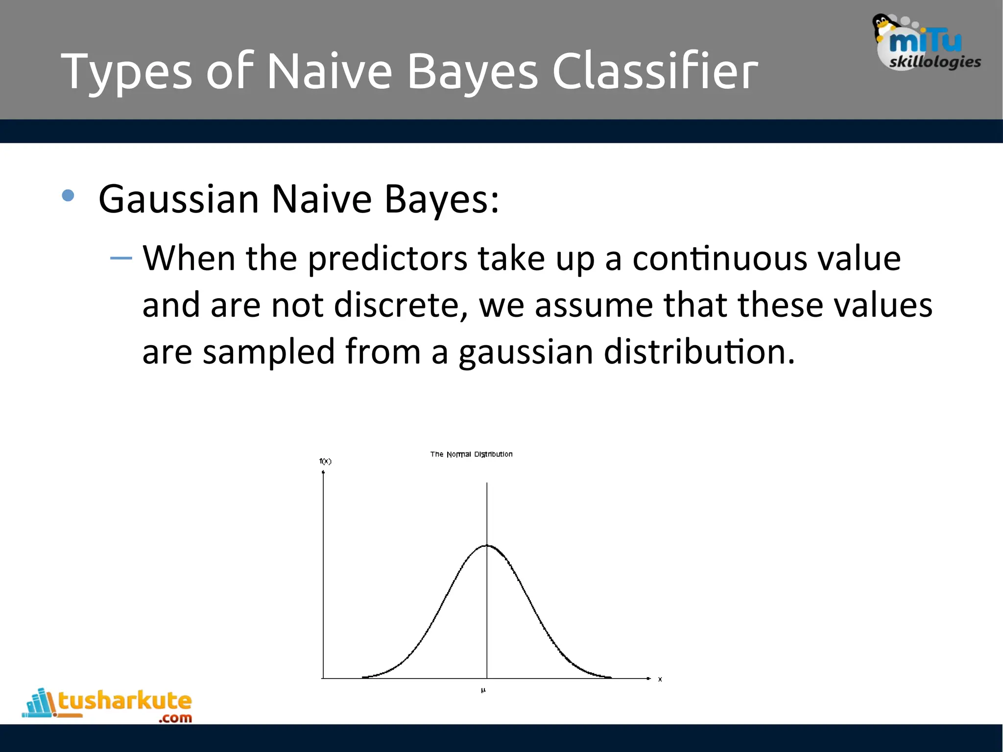
• Gaussian Naive Bayes:
– When the predictors take up a continuous value
and are not discrete, we assume that these values
are sampled from a gaussian distribution.

35. Advantages
• When assumption of independent predictors
holds true, a Naive Bayes classifier performs
better as compared to other models.
• Naive Bayes requires a small amount of
training data to estimate the test data. So, the
training period is less.
• Naive Bayes is also easy to implement.

36. Disadvantages
• Main imitation of Naive Bayes is the assumption of
independent predictors. Naive Bayes implicitly assumes
that all the attributes are mutually independent. In real life,
it is almost impossible that we get a set of predictors which
are completely independent.
• If categorical variable has a category in test data set, which
was not observed in training data set, then model will
assign a 0 (zero) probability and will be unable to make a
prediction. This is often known as Zero Frequency. To solve
this, we can use the smoothing technique. One of the
simplest smoothing techniques is called Laplace estimation.

37. tushar@tusharkute.com
Thank you
This presentation is created using LibreOffice Impress 5.1.6.2, can be used freely as per GNU General Public License
Web Resources
https://mitu.co.in
http://tusharkute.com
/mITuSkillologies @mitu_group
contact@mitu.co.in
/company/mitu-
skillologies
MITUSkillologies