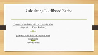
Multivariate Analysis to Will Die When
Mohammed Alharbi
Hap 464
Objective and the objective of the work
Analysis to Predict Who Will Die When.
HOW ?
 Create Training and Validation set .
 Use the training set to calculate likelihood ratio.
 It’s important because it gives forecast information regarding health outcomes.
 this assignment teaching us to explore data and locate exact information among
data.l
Data source
Number of cases
What is the distribution of the data
• Data source from the Assignment
Select count (*) from dbo.final
• The total number of cases
( 17,443,442 number of cases)
• distribution of the data
The average is Average -59.5318
And the Standard deviation- 4.2931
Average AgeAtDx: 59.53186
Standard Deviation of AgeAtDx: 4.293136
Start Dataset (hap464.dbo.final): 17,443,442 Cases
and 829,827 IDs
Zombies Removed: 17,432,694 Cases and 829,659
IDs
>365 Dx/Yr Removed: 17,379,218 Cases and
829,603 IDs  This is your clean data.
80% Training Set From Clean Data: 13,760,416 Cases
and 657,905 IDs
20% Validation Set From Clean Data: 3,619,297
Cases and 171,698 IDs
Preparation of the data
17,443,442
10,748
diagnoses
removed
53,476
diagnoses
removed
829,827 distinct
IDs
Remove
Zombies: 168
distinct IDs
Calculating Likelihood Ratios
(Patients who died within six months after
diagnosis Dead Patients)
(Patients who lived six months after
diagnosis)
Alive Patients
Examples of 10 most deadly and 10 least
deadly diseases
10 Most Deadly:
Icd9 PtsDead6 PtsAlive6 Dead Alive LR
• 1 I218.9 2 2214 112710 545175 0.004369
• 2 I626.2 2 1972 112710 545175 0.004906
• 3 I478.0 2 1183 112710 545175 0.008177
• 4 I599.7 1 544 112710 545175 0.008891
• 5 I620.2 2 773 112710 545175 0.012515
• 6 I717.83 1 349 112710 545175 0.01386
• 7 I474.00 1 343 112710 545175 0.014102
• 8 I296.42 1 338 112710 545175 0.014311
• 9 I716.17 1 338 112710 545175 0.014311
• 10 IV57.22 21 6150 112710 545175 0.016516
• 10 Least Deadly:
icd9 PtsDead6 PtsAlive6 Dead Alive LR
• 1 I853.05 3 1 112710 545175 14.51091
• 2 I798.2 3 1 112710 545175 14.51091
• 3 I183.2 2 1 112710 545175 9.673942
• 4 I798.9 2 1 112710 545175 9.673942
• 5 I194.8 2 1 112710 545175 9.673942
• 6 I960.7 2 1 112710 545175 9.673942
• 7 I862.21 2 1 112710 545175 9.673942
• 8 I852.05 2 1 112710 545175 9.673942
• 9 I718.59 2 1 112710 545175 9.673942
• 10 I531.21 2 1 112710 545175 9.673942
Usefulness of the project
• The usefulness of the project is to practice doing SQL in a large data set by using the skills of
codes, Also to figure out Selecting appropriate method of data analysis and removal of
confounding in the data, Visually present complex multivariate data and Interpret
quantitative findings and relate it to specific policy issues or management decisions.
• In fact, It’s important in our future work filed

Mohammed alharbi 2 e

  • 1.
    Multivariate Analysis toWill Die When Mohammed Alharbi Hap 464
  • 2.
    Objective and theobjective of the work Analysis to Predict Who Will Die When. HOW ?  Create Training and Validation set .  Use the training set to calculate likelihood ratio.  It’s important because it gives forecast information regarding health outcomes.  this assignment teaching us to explore data and locate exact information among data.l
  • 3.
    Data source Number ofcases What is the distribution of the data • Data source from the Assignment Select count (*) from dbo.final • The total number of cases ( 17,443,442 number of cases) • distribution of the data The average is Average -59.5318 And the Standard deviation- 4.2931 Average AgeAtDx: 59.53186 Standard Deviation of AgeAtDx: 4.293136 Start Dataset (hap464.dbo.final): 17,443,442 Cases and 829,827 IDs Zombies Removed: 17,432,694 Cases and 829,659 IDs >365 Dx/Yr Removed: 17,379,218 Cases and 829,603 IDs  This is your clean data. 80% Training Set From Clean Data: 13,760,416 Cases and 657,905 IDs 20% Validation Set From Clean Data: 3,619,297 Cases and 171,698 IDs
  • 4.
    Preparation of thedata 17,443,442 10,748 diagnoses removed 53,476 diagnoses removed 829,827 distinct IDs Remove Zombies: 168 distinct IDs
  • 5.
    Calculating Likelihood Ratios (Patientswho died within six months after diagnosis Dead Patients) (Patients who lived six months after diagnosis) Alive Patients
  • 6.
    Examples of 10most deadly and 10 least deadly diseases 10 Most Deadly: Icd9 PtsDead6 PtsAlive6 Dead Alive LR • 1 I218.9 2 2214 112710 545175 0.004369 • 2 I626.2 2 1972 112710 545175 0.004906 • 3 I478.0 2 1183 112710 545175 0.008177 • 4 I599.7 1 544 112710 545175 0.008891 • 5 I620.2 2 773 112710 545175 0.012515 • 6 I717.83 1 349 112710 545175 0.01386 • 7 I474.00 1 343 112710 545175 0.014102 • 8 I296.42 1 338 112710 545175 0.014311 • 9 I716.17 1 338 112710 545175 0.014311 • 10 IV57.22 21 6150 112710 545175 0.016516 • 10 Least Deadly: icd9 PtsDead6 PtsAlive6 Dead Alive LR • 1 I853.05 3 1 112710 545175 14.51091 • 2 I798.2 3 1 112710 545175 14.51091 • 3 I183.2 2 1 112710 545175 9.673942 • 4 I798.9 2 1 112710 545175 9.673942 • 5 I194.8 2 1 112710 545175 9.673942 • 6 I960.7 2 1 112710 545175 9.673942 • 7 I862.21 2 1 112710 545175 9.673942 • 8 I852.05 2 1 112710 545175 9.673942 • 9 I718.59 2 1 112710 545175 9.673942 • 10 I531.21 2 1 112710 545175 9.673942
  • 7.
    Usefulness of theproject • The usefulness of the project is to practice doing SQL in a large data set by using the skills of codes, Also to figure out Selecting appropriate method of data analysis and removal of confounding in the data, Visually present complex multivariate data and Interpret quantitative findings and relate it to specific policy issues or management decisions. • In fact, It’s important in our future work filed