Bioinformatics

1. Introduction to survival/event
history models

2. Types of outcome
Continuous Ordinary least squares (OLS)
Linear regression
Binary Binary regression
Logistic or probit regression
Time to event data Survival or event history analysis
Ordinary least squares (OLS) regression is an optimization strategy used in linear
regression models that finds a straight line that fits as close as possible to the
data points, in order to help estimate the relationship between a dependent
variable and one or more independent variables.

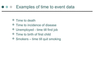
3. Examples of time to event data
 Time to death
 Time to incidence of disease
 Unemployed - time till find job
 Time to birth of first child
 Smokers – time till quit smoking

4. Time to event data
 Analyse durations or length of time to reach
endpoint
 Data are usually censored
 Don’t follow sample long enough for everyone to get to the
endpoint (e.g. death)

5. 4 key concepts for survival analysis
 States
 Events
 Risk period
 Duration

6. States
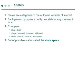
 States are categories of the outcome variable of interest
 Each person occupies exactly one state at any moment in
time
 Examples
 alive, dead
 single, married, divorced, widowed
 never smoker, smoker, ex-smoker
 Set of possible states called the state space

7. Events
 A transition from one state to another
 From an origin state to a destination state
 Possible events depend on the state space
 Examples
 From smoker to ex-smoker
 From married to widowed
 Not all transitions can be events
 E.g. from smoker to never smoker

8. Risk period
 Not all people can experience each state throughout the
study period
 To be able to have a particular event, one must be in the
origin state at some stage
 Example
 can only experience divorce if married
 The period of time that someone is at risk of a particular
event is called the risk period
 All subjects at risk of an event at a point in time called
the risk set

9. Duration
 Event history analysis is to do with the analysis of the
duration of a nonoccurrence of an event or the length of
time during the risk period
 Examples
 Duration of marriage
 Length of life
 In practice we model the probability of a transition
conditional on being in the risk set

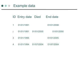
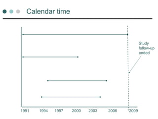
10. Example data
ID Entry date Died End date
1 01/01/1991 01/01/2008
2 01/01/1991 01/01/2000 01/01/2000
3 01/01/1995 01/01/2005
4 01/01/1994 01/07/2004 01/07/2004

11. Calendar time
1991 1994 1997 2000 2003 2006 2009
Study
follow-up
ended

12. Study time in years
0 3 6 9 12 15 18
censored
event
censored
event

13. Censoring
 An observation is censored if it has incomplete
information
 We will only consider right censoring
 That is, the person did not have an event during the time
that they were studied
 Common reasons for right censoring
 the study ends
 the person drops-out of the study
 the person has to be taken off a drug

14. Data
 Survival or event history data
characterised by 2 variables
 Time or duration of risk period
 Failure (event)
• 1 if not survived or event observed
• 0 if censored or event not yet occurred

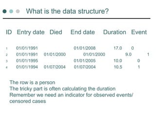
15. What is the data structure?
ID Entry date Died End date Duration Event
1 01/01/1991 01/01/2008 17.0 0
2 01/01/1991 01/01/2000 01/01/2000 9.0 1
3 01/01/1995 01/01/2005 10.0 0
4 01/01/1994 01/07/2004 01/07/2004 10.5 1
The row is a person
The tricky part is often calculating the duration
Remember we need an indicator for observed events/
censored cases

16. Worked example
 Random 20% sample from BHPS
 Waves 1 – 15
 One record per person/wave
 Outcome: Duration of cohabitation
 Conditions on cohabiting in first wave
 Survival time: years from entry to the study in 1991
till year living without a partner

17. The data
+----------------------------+
| pid wave mastat |
|----------------------------|
| 10081798 1 married |
| 10081798 2 married |
| 10081798 3 married |
| 10081798 4 married |
| 10081798 5 married |
| 10081798 6 married |
| 10081798 7 widowed |
| 10081798 8 widowed |
| 10081798 9 widowed |
| 10081798 10 widowed |
| 10081798 11 widowed |
| 10081798 12 widowed |
| 10081798 13 widowed |
| 10081798 14 widowed |
| 10081798 15 widowed |
|----------------------------|
Duration = 6 years
Event = 1
Ignore data after
event = 1

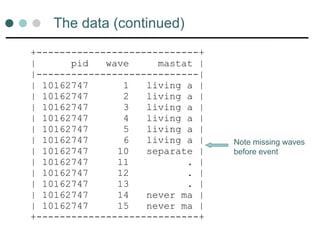
18. The data (continued)
+----------------------------+
| pid wave mastat |
|----------------------------|
| 10162747 1 living a |
| 10162747 2 living a |
| 10162747 3 living a |
| 10162747 4 living a |
| 10162747 5 living a |
| 10162747 6 living a |
| 10162747 10 separate |
| 10162747 11 . |
| 10162747 12 . |
| 10162747 13 . |
| 10162747 14 never ma |
| 10162747 15 never ma |
+----------------------------+
Note missing waves
before event

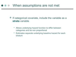
19. Preparing the data
. sort pid wave
. generate skey=1 if wave==1&(mastat==1|mastat==2)
. by pid: replace skey=skey[_n-1] if wave~=1
. keep if skey==1
. drop skey
.
. stset wave,id(pid) failure(mastat==3/6)
id: pid
failure event: mastat == 3 4 5 6
obs. time interval: (wave[_n-1], wave]
exit on or before: failure
------------------------------------------------------------------------------
15058 total obs.
1628 obs. begin on or after (first) failure
------------------------------------------------------------------------------
13430 obs. remaining, representing
1357 subjects
270 failures in single failure-per-subject data
13612 total analysis time at risk, at risk from t = 0
earliest observed entry t = 0
last observed exit t = 15
Select records for
respondents who
were cohabiting in 1991
Declare that you want to
set the data to survival time
Important to check that you
have set data as intended

20. Checking the data setup
. list pid wave mastat _st _d _t _t0 if pid==10081798,sepby(pid) noobs
+-------------------------------------------------+
| pid wave mastat _st _d _t _t0 |
|-------------------------------------------------|
| 10081798 1 married 1 0 1 0 |
| 10081798 2 married 1 0 2 1 |
| 10081798 3 married 1 0 3 2 |
| 10081798 4 married 1 0 4 3 |
| 10081798 5 married 1 0 5 4 |
| 10081798 6 married 1 0 6 5 |
| 10081798 7 widowed 1 1 7 6 |
| 10081798 8 widowed 0 . . . |
| 10081798 9 widowed 0 . . . |
| 10081798 10 widowed 0 . . . |
| 10081798 11 widowed 0 . . . |
| 10081798 12 widowed 0 . . . |
| 10081798 13 widowed 0 . . . |
| 10081798 14 widowed 0 . . . |
| 10081798 15 widowed 0 . . . |
+-------------------------------------------------+
1 if observation is to be used
and 0 otherwise
1 if event, 0 if censoring or
event not yet occurred
time of exit
time of entry

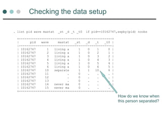
21. Checking the data setup
. list pid wave mastat _st _d _t _t0 if pid==10162747,sepby(pid) noobs
+--------------------------------------------------+
| pid wave mastat _st _d _t _t0 |
|--------------------------------------------------|
| 10162747 1 living a 1 0 1 0 |
| 10162747 2 living a 1 0 2 1 |
| 10162747 3 living a 1 0 3 2 |
| 10162747 4 living a 1 0 4 3 |
| 10162747 5 living a 1 0 5 4 |
| 10162747 6 living a 1 0 6 5 |
| 10162747 10 separate 1 1 10 6 |
| 10162747 11 . 0 . . . |
| 10162747 12 . 0 . . . |
| 10162747 13 . 0 . . . |
| 10162747 14 never ma 0 . . . |
| 10162747 15 never ma 0 . . . |
+--------------------------------------------------+
How do we know when
this person separated?

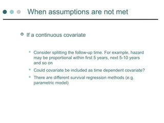
22. Trying again!
. fillin pid wave
. stset wave,id(pid) failure(mastat==3/6) exit(mastat==3/6 .)
id: pid
failure event: mastat == 3 4 5 6
obs. time interval: (wave[_n-1], wave]
exit on or before: mastat==3 4 5 6 .
---------------------------------------------------------------------------
---
20355 total obs.
7524 obs. begin on or after exit
---------------------------------------------------------------------------
---
12831 obs. remaining, representing
1357 subjects
234 failures in single failure-per-subject data
12831 total analysis time at risk, at risk from t = 0
earliest observed entry t = 0
last observed exit t = 15

23. . list pid wave mastat _st _d _t _t0 if pid==10162747,sepby(pid) noobs
+--------------------------------------------------+
| pid wave mastat _st _d _t _t0 |
|--------------------------------------------------|
| 10162747 1 living a 1 0 1 0 |
| 10162747 2 living a 1 0 2 1 |
| 10162747 3 living a 1 0 3 2 |
| 10162747 4 living a 1 0 4 3 |
| 10162747 5 living a 1 0 5 4 |
| 10162747 6 living a 1 0 6 5 |
| 10162747 7 . 1 0 7 6 |
| 10162747 8 . 0 . . . |
| 10162747 9 . 0 . . . |
| 10162747 10 separate 0 . . . |
| 10162747 11 . 0 . . . |
| 10162747 12 . 0 . . . |
| 10162747 13 . 0 . . . |
| 10162747 14 never ma 0 . . . |
| 10162747 15 never ma 0 . . . |
+--------------------------------------------------+
Checking the new data setup
Now censored instead of
an event

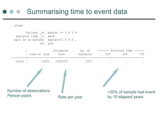
24. Summarising time to event data
 Individuals followed up for different lengths of time
 So can’t use prevalence rates (% people who have
an event)
 Use rates instead that take account of person years
at risk
 Incidence rate per year
 Death rate per 1000 person years

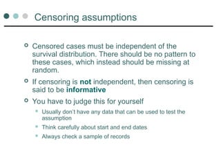
25. Summarising time to event data
Number of observations
Person-years Rate per year
<25% of sample had event
by 15 elapsed years
. stsum
failure _d: mastat == 3 4 5 6
analysis time _t: wave
exit on or before: mastat==3 4 5 6 .
id: pid
| incidence no. of |------ Survival time -----|
| time at risk rate subjects 25% 50% 75%
---------+---------------------------------------------------------------------
total | 12831 .0182371 1357 . . .

26. List the cumulative hazard function
Default is the survivor function
. sts list, failure
failure _d: mastat == 3 4 5 6
analysis time _t: wave
exit on or before: mastat==3 4 5 6 .
id: pid
Beg. Net Failure Std.
Time Total Fail Lost Function Error [95% Conf. Int.]
-------------------------------------------------------------------------------
2 1357 29 162 0.0214 0.0039 0.0149 0.0306
3 1166 33 89 0.0491 0.0061 0.0384 0.0625
4 1044 16 64 0.0636 0.0070 0.0513 0.0789
5 964 35 58 0.0976 0.0088 0.0818 0.1164
6 871 12 34 0.1101 0.0094 0.0931 0.1300
7 825 20 24 0.1316 0.0103 0.1128 0.1534
8 781 14 17 0.1472 0.0109 0.1271 0.1701
9 750 12 30 0.1609 0.0115 0.1398 0.1848
10 708 15 23 0.1786 0.0121 0.1563 0.2038
11 670 9 32 0.1897 0.0125 0.1666 0.2155
12 629 8 16 0.2000 0.0128 0.1762 0.2266
13 605 13 24 0.2172 0.0134 0.1922 0.2449
14 568 8 24 0.2282 0.0138 0.2025 0.2566
15 536 10 526 0.2426 0.0143 0.2160 0.2719
-------------------------------------------------------------------------------

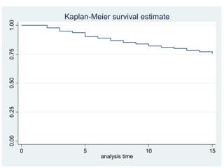
27. Graphs of survival time
 Kaplan-Meier estimate of survival curve
 The Kaplan-Meier method estimates the cumulative
probability of an individual surviving after baseline to
any time, t

28. 0.00
0.25
0.50
0.75
1.00
0 5 10 15
analysis time
Kaplan-Meier survival estimate

29. Kaplan-Meier graphs
 Can read off the estimated probability of surviving a
relationship at any time point on the graph
 E.g. at 5 years 88% are still cohabiting
 The survival probability only changes when an event
occurs
 So the graph is stepped and not a smooth curve

30. 0.00
0.25
0.50
0.75
1.00
0 5 10 15
time in years
Kaplan-Meier survival estimate

31. 0.00
0.25
0.50
0.75
1.00
0 5 10 15
analysis time
sex = male sex = female
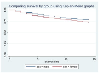
Comparing survival by group using Kaplan-Meier graphs

32. Testing equality of survival curves among
groups
The log-rank test
A non –parametric test that assesses the null
hypothesis that there are no differences in survival
times between groups

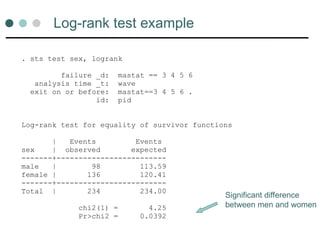
33. . sts test sex, logrank
failure _d: mastat == 3 4 5 6
analysis time _t: wave
exit on or before: mastat==3 4 5 6 .
id: pid
Log-rank test for equality of survivor functions
| Events Events
sex | observed expected
-------+-------------------------
male | 98 113.59
female | 136 120.41
-------+-------------------------
Total | 234 234.00
chi2(1) = 4.25
Pr>chi2 = 0.0392
Log-rank test example
Significant difference
between men and women

34. The Cox regression model

35. Event History with Cox Model
Event History with Cox regression model
 No longer modelling the duration
 Modelling the hazard
 Hazard: measure of the probability that an event
occurs at time t conditional on it not having occurred
up until t
 Also known as the Cox proportional hazard model

36. Some hazard shapes
 Increasing
 Onset of Alzheimer's
 Decreasing
 Survival after surgery
 U-shaped
 Age specific mortality
 Constant
 Time till next email arrives

37. Cox regression model
 Regression model for survival analysis
 Can model time invariant and time varying
explanatory variables
 Produces estimated hazard ratios (sometimes
called rate ratios or risk ratios)
 Regression coefficients are on a log scale
 Exponentiate to get hazard ratio
 Similar to odds ratios from logistic models

38. Cox regression equation
)
.......
exp(
)
(
)
( 2
2
1
1
0 in
n
i
i
i x
x
x
t
h
t
h 

 



)
(
0 t
h
)
(t
hi
is the baseline hazard function and can take any
form
It is estimated from the data (non parametric)
is the hazard function for individual i
in
i
i x
x
x ,....,
, 2
1
n


 ,....,
, 2
1
are the covariates
are the regression coefficients estimated from the data
Effect of covariates is constant over time (parameterised)
This is the proportional hazards assumption
Therefore, Cox regression referred to as a semi-parametric

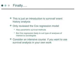
39. Cox regression in Stata
 Will first model a time invariant covariate (sex)
on risk of partnership ending
 Then will add a time dependent covariate (age)
to the model

40. Cox regression in Stata
. stcox female
failure _d: mastat == 3 4 5 6
analysis time _t: wave
exit on or before: mastat==3 4 5 6 .
id: pid
Cox regression -- Breslow method for ties
No. of subjects = 1357 Number of obs = 12337
No. of failures = 234
Time at risk = 12337
LR chi2(1) = 4.18
Log likelihood = -1574.5782 Prob > chi2 = 0.0409
------------------------------------------------------------------------------
_t | Haz. Ratio Std. Err. z P>|z| [95% Conf. Interval]
-------------+----------------------------------------------------------------
female | 1.30913 .1734699 2.03 0.042 1.009699 1.697358
------------------------------------------------------------------------------

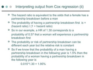
41. Interpreting output from Cox regression
 Cox model has no intercept
 It is included in the baseline hazard
 In our example, the baseline hazard is when sex=1 (male)
 The hazard ratio is the ratio of the hazard for a unit
change in the covariate
 HR = 1.3 for women vs. men
 The risk of partnership breakdown is increased by 30% for women
compared with men
 Hazard ratio assumed constant over time
 At any time point, the hazard of partnership breakdown for a woman
is 1.3 times the hazard for a man

42. Interpreting output from Cox regression (ii)
 The hazard ratio is equivalent to the odds that a female has a
partnership breakdown before a man
 The probability of having a partnership breakdown first is =
(hazard ratio) / (1 + hazard ratio)
 So in our example, a HR of 1.30 corresponds to a
probability of 0.57 that a woman will experience a partnership
breakdown first
 The probability or risk of partnership breakdown can be
different each year but the relative risk is constant
 So if we know that the probability of a man having a
partnership breakdown in the following year is 1.5% then the
probability of a woman having a partnership breakdown in
the following year is
0.015*1.30 = 1.95%

43. 0
.05
.1
.15
.2
.25
0 5 10 15
_t
sex = women sex = men
Estimated cumulative hazard: men vs. women

44. .012
.014
.016
.018
.02
Smoothed
hazard
function
4 6 8 10 12
analysis time
hazard function varying over time
Cox proportional hazards regression:

45. Time dependent covariates
 Examples
 Current age group rather than age at baseline
 GHQ score may change over time and predict break-ups
 Will use age to predict duration of cohabitation
 Nonlinear relationship hypothesised
 Recode age into 8 equally spaced age groups

46. Cox regression with time dependent covariates
. xi: stcox female i.agecat
i.agecat _Iagecat_0-7 (naturally coded; _Iagecat_0 omitted)
failure _d: mastat == 3 4 5 6
analysis time _t: wave
exit on or before: mastat==3 4 5 6 .
id: pid
Cox regression -- Breslow method for ties
No. of subjects = 1357 Number of obs = 12337
No. of failures = 234
Time at risk = 12337
LR chi2(8) = 78.44
Log likelihood = -1537.4472 Prob > chi2 = 0.0000
------------------------------------------------------------------------------
_t | Haz. Ratio Std. Err. z P>|z| [95% Conf. Interval]
-------------+----------------------------------------------------------------
female | 1.3705 .1842481 2.34 0.019 1.05304 1.783666
_Iagecat_1 | .5838602 .1883578 -1.67 0.095 .3102449 1.098786
_Iagecat_2 | .311325 .1039311 -3.50 0.000 .1618279 .5989281
_Iagecat_3 | .2136714 .0737986 -4.47 0.000 .1085813 .4204725
_Iagecat_4 | .2225187 .0811395 -4.12 0.000 .1088888 .4547261
_Iagecat_5 | .4770023 .1691695 -2.09 0.037 .238035 .9558732
_Iagecat_6 | 1.203702 .4306775 0.52 0.604 .5969856 2.427023
_Iagecat_7 | 1.644141 .9677715 0.84 0.398 .518688 5.21161
------------------------------------------------------------------------------

47. Cox regression assumptions
 Assumption of proportional hazards
 No censoring patterns
 True starting time
 Plus assumptions for all modelling
 Sufficient sample size, proper model specification, independent
observations, exogenous covariates, no high multicollinearity,
random sampling, and so on

48. Proportional hazards assumption
 Cox regression with time-invariant covariates
assumes that the ratio of hazards for any two
observations is the same across time periods
 This can be a false assumption, for example
using age at baseline as a covariate
 If a covariate fails this assumption
 for hazard ratios that increase over time for that covariate,
relative risk is overestimated
 for ratios that decrease over time, relative risk is
underestimated
 standard errors are incorrect and significance tests are
decreased in power

49. Testing the proportional hazards assumption
 Graphical methods
 Comparison of Kaplan-Meier observed & predicted curves
by group. Observed lines should be close to predicted
 Survival probability plots (cumulative survival against time
for each group). Lines should not cross
 Log minus log plots (minus log cumulative hazard against
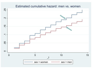
log survival time). Lines should be parallel

50. Testing the proportional hazards assumption
 Formal tests of proportional hazard
assumption
 Include an interaction between the covariate and a function
of time. Log time often used but could be any function. If
significant then assumption violated
 Test the proportional hazards assumption on the basis of
partial residuals. Type of residual known as Schoenfeld
residuals.

51. When assumptions are not met
 If categorical covariate, include the variable as a
strata variable
 Allows underlying hazard function to differ between
categories and be non proportional
 Estimates separate underlying baseline hazard for each
stratum

52. When assumptions are not met
 If a continuous covariate
 Consider splitting the follow-up time. For example, hazard
may be proportional within first 5 years, next 5-10 years
and so on
 Could covariate be included as time dependent covariate?
 There are different survival regression methods (e.g.
parametric model)

53. Censoring assumptions
 Censored cases must be independent of the
survival distribution. There should be no pattern to
these cases, which instead should be missing at
random.
 If censoring is not independent, then censoring is
said to be informative
 You have to judge this for yourself
 Usually don’t have any data that can be used to test the
assumption
 Think carefully about start and end dates
 Always check a sample of records

54. True starting time
 The ideal model for survival analysis would be
where there is a true zero time
 If the zero point is arbitrary or ambiguous, the
data series will be different depending on
starting point. The computed hazard rate
coefficients could differ, sometimes markedly
 Conduct a sensitivity analysis to see how
coefficients may change according to different
starting points

55. Other extensions to survival analysis
 Discrete (interval-censored) survival times
 Repeated events
 Multi-state models (more than 1 event type)
 Transition from employment to unemployment or leaving
labour market
 Modelling type of exit from cohabiting relationship-
separation/divorce/widowhood

56. Could you use logistic regression
instead?
 May produce similar results for short or fixed
follow-up periods
 Examples
• everyone followed-up for 7 years
• maximum follow-up 5 years
 Results may differ if there are varying follow-up
times
 If dates of entry and dates of events are
available then better to use Cox regression

57. Finally….
 This is just an introduction to survival/ event
history analysis
 Only reviewed the Cox regression model
 Also parametric survival methods
 But Cox regression likely to suit type of analyses of
interest to sociologists
 Consider an intensive course if you want to use
survival analysis in your own work

58.  Thank you!