Learning Objectives
Session 1:
Sequencingtechnologies and NGS Overview
Part 1: Introduction to DNA Sequencing
Part 2: DNA Sequencing in the NGS era
Part 3: Overview of NGS Technologies
Part 4: DNA-Seq
‐ Protocol : Overview
Part 5: DNA-Seq
‐ Analysis Pipeline and File Formats
Introduction to Bioinformatics
Genomics| Dr KONATE
3.
Learning Outcomes
Session 1:
Sequencingtechnologies and NGS Overview
Understand basics of NGS technologies
Understand different NGS file formats
Navigate through database repositories to retrieve
NGS datasets
Introduction to Bioinformatics
Genomics| Dr KONATE
What is DNASequencing ?
DNA Sequencing is the process of reading the
nucleotides present in DNA : determining the precise
order of nucleotides within a DNA molecule.
DNA-Seq
‐ generally refers today to any NGS method
or technology that is used to determine the order of
the four bases (A, T, C, G) in a strand of DNA.
Introduction to Bioinformatics
Genomics| Dr KONATE
6.
What is DNASequencing ?
In fact, there are 2 main types of DNA sequencing
technologies that are used today: Sanger sequencing
and Next-Generation
‐ Sequencing (NGS).
Each of these technologies has utility in today’s
genetic analysis environment.
Introduction to Bioinformatics
Genomics| Dr KONATE
7.
1953
(Watson & Crick)
DNAStructure as a
double helix
1972-1976
‐
(Min Jou et al., 1972; Fiers
et al., 1976) sequence of the
1st complete gene and the
complete genome of
Bacteriophage MS2 (viral
RNA 3,569 nt)
1977
(Sanger et al., Feb 1977)
The first full DNA genome to
be sequenced :
bacteriophage φX174
1977
Maxam & Gilbert
+ Sanger sequencing
1987
ABI markets ABI370,
the 1st fully automated
sequencing machine
1995
(C.Venter) 1st complete genome
of a free-living
‐ organism, the
bacterium H. influenzae
(circular chr >1,8Mb)
1995
First published use
of WGS sequencing
1996
First NGS technology :
2001
Draft sequence of the human
genome (shotgun sequencing
methods). Public & Private (Lander et
al., Feb 2001 Nature; Venter et al.,
Feb 2001 Science)
Introd
Pyrosequencing uction to Bioinformatics
Genomics| Dr KONATE
Main DNA sequencing technologies
8.
The Human GenomeProject:
the objectives
The Human Genome Project (HGP)= a 13-years
‐ (1990-April
‐ 14, 2003)
international effort to sequence of the 3 billion "letters” of human DNA.
$300 million project, led by the U.S. DoE and the NIH.
International Human Genome Sequencing Consortium (IHGSC)= group of
publicly funded researchers
At any given time, ≈ 200 labs in the United States supported these
efforts +
> 18 different countries from across the globe had contributed to the
HGP.
Chial, 2008 http://www.genome.gov/sequencingcosts/
Introduction to Bioinformatics
OnwlinwewC.soanugresre.a:IcB.uTk
Genomics| Dr KONATE
9.
The Human GenomeProject:
the objectives
2 groups competing for sequencing:
-
‐ Public
-
‐ Private (Celera Genomics)
Opposing philosophies :
-
‐ HGP Bermuda Agreement (1996)
all information from the project would be
made freely available to all within 24h.
-
‐ Private
access restricted to paying customers !
In February 2001, drafts of the human genome
sequence were published simultaneously by both
public-private
‐ groups in separate articles (Lander et al
(IHGSC)., Feb 2001 Nature; Venter et al., Feb 2001 Science). Chial, 2008
http://www.genome.gov/sequencingcosts/
http://ww
w.yourgen
ome.org/
Introduction to Bioinformatics Onliwnwe
wCo.suarnsgee:rI.BaTc.uk
Genomics| Dr KONATE
10.
The Human GenomeProject:
the method (WGS)
Hierarchical genome shotgun sequencing
-
‐ Shotgun phase
Genome fragmented into larger segments
cloning into vectors
clones sequencing
shotgun sequences assembly
relied on the physical map of the human genome
established earlier.
-
‐ Finishing phase : filling in gaps and resolving DNA
sequences in ambiguous areas
Whole-genome
‐ shotgun sequencing
(Celera genomics)
Genome sheared randomly into small fragments
(appropriately sized for sequencing)
Reassembly.
The IHGSC and Celera used the same general
method of termination chain for the DNA
Introduction to Bioinformatics
sequencing (Hood & Galas, 2003).
Genomics| Dr KONATE
11.
Sequencing Quality
Sequencing qualitydepend upon the average number of times each base
in the genome is 'read' during the sequencing process.
For the Human Genome Project (HGP) :
-
‐ 'draft sequence' (covering ~90% of the genome at ~99.9% accuracy)
-
‐ 'finishedsequence' (covering >95% of
the genome at ~99.99% accuracy).
Producing truly high-quality
‐ 'finished' sequence by this definition is very
expensive and labor-intensive.
‐
Several releases of the human genome sequences
Introductih
ott
np:
t/
o/
w
Bw
iow
in.g
fe
on
rmom
ae
ti.
cg
sov
O/
nse
liq
nu
ee
Cn
oci
un
rg
sc
eo
:s
It
Bs
T/
12.
Finished Genome vsDraft Genome
Variable degrees of completion of published genomes
Draft Sequencing
-
‐ high-throughput
‐ or shotgun phase (whole genome or clone-based
‐ approach)
-
‐ Assembly using specific algorithms (whole-genome
‐ or single-clone
‐ assembly)
lower accuracy than finished sequence; some segments are missing or in
the wrong order or orientation.
Finishing
-
‐ Accuracy in bases identification + Quality Check + few if any gaps.
-
‐ Contiguous segments of sequence are ordered and linked to one another
-
‐ No ambiguities or discrepancies about segments order and orientation
Complete Genome
A Genome represented by a single contiguous sequence with no ambiguities
The sequences available are finished to a certain high quality.
(Mardis et al., 2002)
Introduction to
Bioinhfttoprm://awtiwcswO.innfloinrme
aCtiocusr.
jsaex:.IoBrTg
/
13.
The Human GenomeProject:
the heritage
The HGP project required that all human genome sequence information be
freely and publicly available. The existing DNA sequences have been stored
in databases available to anyone willing to exploit and analyze them.
Dedicated databases house various data for model organisms such as
sequences of known and hypothetical genes and proteins (GenBank, NCBI).
Other databases (Ensembl http://www.ensembl.org) present additional data
and annotation as well as powerful tools for visualizing and searching it.
Community efforts for non-model
‐ organisms like Eukaryotic Pathogens :
EuPathDB (http://eupathdb.org/eupathdb/).
Computer programs have been developed to analyze and interpret the data.
Introduction to Bioinformatics
Genomics| Dr KONATE
14.
The Human GenomeProject:
the heritage
The human genome contains only
about 20,000 protein-coding
‐ genes,
similar in number and with largely
orthologous functions as those in
nematodes that have only 1,000
somatic cells.
The extent of non-protein-
‐ coding
‐
DNA increases with increasing
complexity, reaching > 98% in
humans.
Encode
Gencode
Introduction to Bioinformatics
Online(M
Ca
otti
uc
rk
s,
e2
:0
IB11
T)
Genomics| Dr KONATE
15.
The Human GenomeProject:
the heritage
Encode (https://www.encodeproject.org)
The Encyclopedia of DNA Elements (ENCODE) Project aims to provide “a list
of functional elements in the human genome, including elements that act at
the protein and RNA levels, and regulatory elements that control cells and
circumstances in which a gene is active. “
“the generation of such a catalogue is crucial for understanding genome
function.”
Gencode (http://www.gencodegenes.org)
The human genome has been the focus of intensive manual annotation:
The GENCODE Consortium aims to identify all gene features in the human
and mouse genomes using a combination of computational analysis, manual
annotation, and experimental validation.
(Djebali et al., 2012)
(Harrow et al., 2012)
Introduction to Bioinformatics O(Bnirlinneey Ceot
ualr.s, e2:0I0B7T)
Genomics| Dr KONATE
16.
The Human GenomeProject:
the heritage
Genetic differences in individual bases (SNPs) of a genome are by far the most
common type of genetic variation.
Goal: develop a Haplotype Map of the Human Genome
= identification and cataloging of most of the millions of SNPs estimated to occur
commonly in the human genome.
Described variants are, their location, their distribution among people within
populations and among populations in different parts of the world. designed to
provide information to link genetic variants to the risk for specific diseases
1000 Genomes Project: has become more complete and reliable as many novel
variants have been discovered !!
Introduction to
Bioinfh
ott
rmp:/
a/
tiha
cp
sm
Oa
np
l.
in
nc
ebi.
Cn
olm
u.
rn
si
eh.
:g
IBov
T
17.
Introduction to Bioinformatics
hGttep:n//ohmapicmsa|
p.Fnactbmi.nalmG.nuieh.rgfoavli
TheHuman Genome Project:
the heritage
1000 Genomes (www.1000genomes.org/)
►identify most genetic variants with frequencies of at least 1%.
►freely accessible ressource of human genetic variation.
►final data set = data for 2,504 individuals from 26
populations. (low coverage sequencing and exome sequence
data for all)
►International Genome Sample Resource (IGSR) for ongoing
usability of data generated by the 1000 Genomes Project.
UK10K (www.uk10k.org/)
►identification of rare genetic variants through the study of
the DNA of 4,000 individuals and their comparison to the
protein-
‐ coding areas of 6,000 people with documented
diseases.
►link between genetic variants and rare diseases.
18.
The Human GenomeProject:
the heritage
Development of novel technologies to help increase the depth of
sequencing: Next-Generation
‐ Sequencing (NGS) technologies
Since their development, NGS technologies have gained increasing
attention with a considerable potential application in both diagnostic and
public health microbiology.
Revolutionized the sequencing process: from Sanger to HT sequencing
(Salipante et al., 2013)
Introduction to Bioinformatics
Genomics| Dr KONATE
DNA Sequencing method:
fromSanger to NGS
Sanger sequencing is the method developed by Frederick Sanger in 1977.
This method involves copying single-stranded
‐ DNA with chemically altered
bases called dideoxynucleotides (ddNTPs).
ddNTPs when incorporated at the 3' end of the growing chain, terminate the
chain selectively at A, C, G, or T. The terminated chains are then resolved by
capillary electrophoresis.
Introduction to Bioinformatics Online Course
www.the-
scientist.c:oIBmT
Genomics| Dr KONATE
21.
DNA Sequencing method:
fromSanger to NGS
Applied Biosystems (Life Technologies), manufactured the
automated capillary sequencers utilized by both Celera
Genomics and The Human Genome Project.
While capillary sequencing was the first approach to
successfully sequence a full human genome, it was still too
expensive and took too long for commercial purposes !!!
Because of this, sequencing using Sanger technology has been
displaced by technologies like pyrosequencing, or SMRT
sequencing…
Introduction to Bioinformatics
Genomics| Dr KONATE
22.
DNA-Seq
‐
DNA-Seq
‐ is nowadaysused as an effective sequencing strategy
after the advent of rapid DNA sequencing methods that has
greatly accelerated biological and medical research and
discovery : de novo…
DNA-Seq
‐ may be used to determine the sequence of
individual genes, larger genetic regions, full chromosomes, or
entire genomes.
‘DNA-Seq’
‐ and other related ‘seq’ technologies allow to cover
genome complexity : genomic DNA-Seq,
‐ Methyl-Seq,
‐ ChIP-Seq,
‐
exome sequencing…
Introduction to Bioinformatics
Genomics| Dr KONATE
23.
NGS
Next-generation
‐ sequencing (NGS),or high-throughput
‐ (HT)
sequencing = catch-all
‐ term describing different modern
sequencing technologies used by different platforms:
-
‐ Illumina (Solexa) sequencing
-
‐ Roche 454 sequencing
-
‐ Ion torrent: Proton / PGM sequencing
-
‐ …
DNA sequence faster and cheaper than the Sanger sequencing
= revolution for genomics and molecular biology.
Introduction to Bioinformatics
Genomics| Dr KONATE
24.
NGS:
Sequencing Technologies andPlatforms
Technology
Introduction to Bioinformatics
Genomics| Dr KONATE
Company Support Chemistry
Massively Parallel
Sequencing
Solexa
454
SOLiD
Ion
Torren
t
Illumina
Roche Applied Science
AB / Life Technologies
Life Technologies
Bridge PCR on flowcell
emPCR on beads
emPCR on beads
emPCR on beads
Seq-By-
‐ Synthesis
‐
Pyrosequencing
Seq-By-
‐ Ligation
‐
Proton detection
Single Molecule
Sequencing
PacBio SMRT
Nanopore
Pacific Biosciences
Oxford Nanopore Tech/McNally
Pol performance
Translocation
Real-time-
‐ Seq
‐
NA
25.
NGS:
Principles of DNASequencing: SBS
Tracking the addition of labeled nucleotides as the DNA chain is copied
The DNA template is immobilized.
Solutions of A, nucleotides C , G and T sequentially added and removed.
Light is generated when a nucleotide complements the first unpaired base.
Chemiluminescent signal detected to determine the sequence.
Introduction to Bioinformatics Online Course:IBT
Genomics| Dr KONATE
26.
NGS:
In brief :emPCR (454/SOLiD/Ion Torrent) vs Bridge PCR (Illumina)
Bridge PCR
(Shendure & Ji, 2008)
Introduction to Bioinformatics
Genomics| Dr KONATE
-
‐ The adaptor-flanked
‐ shotgun library is PCR amplified on a flow cell
-
‐ both primers coat the surface of a solid substrate
-
‐ Amplification products from any given member of the library
remain locally fixed near the point of origin = cluster
-
‐ The PCR produces clonal clusters contains copies of a single DNA.
27.
NGS:
Introduction to Bioinformatics
Genomics|Dr KONATE
Principles of DNA Sequencing: Pyrosequencing
Incorporation of dNTPs by DNApol releases pyrophosphate (PPi).
ATP sulfurylase converts PPi to ATP in the presence of APS.
ATP = substrate for the luciferase-mediated
‐ conversion of luciferin to oxyluciferin
This conversion generates light in amounts proportional to the amount of ATP
detected by a camera.
Unincorporated nucleotides and ATP are degraded by the apyrase, and the reaction
can restart with another nucleotide
APS : adenosine 5´phosphosulfate
PPi : Pyrophosphate
DNApol: DNA Polymerase
(https://
en.wikipedia.org)
28.
NGS:
In brief :emPCR (454/SOLiD/Ion Torrent) vs Bridge PCR (Illumina)
emPCR
-
‐ The adaptor-flanked
‐ shotgun library is PCR amplified in the context of
a water-
‐ in-oil
‐ emulsion.
-
‐ PCR primer is 5'-attached
‐ on micron-scale
‐ beads.
-
‐ 1 bead-containing
‐ compartments = 0 or 1 template DNA.
-
‐ PCR amplicons are captured to the surface of the bead.
-
‐ 1 clonally amplified bead = PCR products corresponding to
amplification of a single molecule from the library.
(Shendure & Ji, 2008)
Introduction to Bioinformatics
Genomics| Dr KONATE
NGS:
Sequencing Technologies andPlatforms
Technology
Introduction to Bioinformatics
Genomics| Dr KONATE
Company Support Chemistry
Massively Parallel
Sequencing
Solexa
454
SOLiD
Ion
Torren
t
Illumina
Roche Applied Science
AB / Life Technologies
Life Technologies
Bridge PCR on flowcell
emPCR on beads
emPCR on beads
emPCR on beads
Seq-By-
‐ Synthesis
‐
Pyrosequencing
Seq-By-
‐ Ligation
‐
Proton detection
Single Molecule
Sequencing
PacBio SMRT
Nanopore
Pacific Biosciences
Oxford Nanopore Tech/McNally
Pol performance
Translocation
Real-time-
‐ Seq
‐
NA
31.
Solexa
The input samplemust be
cleaved into short sections.
Fragments are ligated to
adaptors and annealed to the
slide using the adaptors.
Fragments are separated into
single strands to be sequenced.
Nucleotides are modified so that
each emits a different coloured
light when excited by a laser.
+ they have a terminator, so that
only one base is added at a time.
PCR, process repeated in cycles,
images analyzed.
Flow cell
Introduction
to(BmiooindfiofiremdatifrcosmOnGlinilechCroiusr
ts,e2:I0B1T0)
454 Technology
As inIllumina, the DNA is fragmented.
Adaptors added, end annealed to beads.
1 DNA fragment = 1 bead.
Fragments amplified by PCR using adaptor-specific
‐ primers.
The sequence can then be determined computationally.
Longer reads than Illumina, different lengths.
Introduction to
Bioinformati(chsttOpn:/l/inwewCwo.eubrsi.ea:cI.BuT
k)
34.
Introduction to Bioinformatics
Genomics|(wFawtwm.a45G4u.ceormfa/l)i
454Technology
Intra-Platform
‐ Comparison
Features combination of long reads, accuracy
and high-throughput, making the system well
suited for larger genomic projects.
brings the power of 454
Sequencing Systems
directly to the laboratory
benchtop
GS FLX+ System
GS Junior System
Read lengths:
GS Junior (up to 400bp)
GS Junior + (700-800bp)
Read lengths:
GS FLX Titanium XL+ (up to 1,000bp)
GS FLX Titanium XLR70 (up to 600bp)
35.
SOLID
In the SOLiDsequencing method, unlike
other NGS technologies (which base
detection of DNA fragments is performed
through polymerase reaction) sequencing
is achieved by Sequencing-By-
‐ Ligation
‐ .
Sequencing is performed with a ligase, rather than a polymerase.
Each sequencing cycle introduces a partially degenerated population of fluorescently
labeled octamers. The population is structured such that the label correlates with the
identity of the central 2 bp in the octamer.
After ligation and imaging in four channels, the labeled portion of the octamer (that is,
'zzz') is cleaved leaving a free end for another cycle of ligation.
Adapted from (Shendure & Ji,
I2n0t0r8o)dauncdti(hottnpt:/o/wBwiowin.sfporirnmgearti.ccosmO/9n7l8in-1
‐ e-
‐
4C6o14u-
‐r7s7e2:5IB-9
‐ T)
Genomics| Dr KONATE
36.
Ion Torrent
As inother kinds of NGS, the input DNA is fragmented.
Adaptors are added and one molecule is placed onto a bead.
Amplification on the bead by emulsion PCR. Each bead is placed into 1 well of a slide.
The pH is detected is each of the wells, as each H+ ion released will decrease the pH.
The changes in pH allow us to determine if that base, and how many thereof, was
added to the sequence read.
The dNTPs are washed away, and the
process is repeated in cycles.
Adapted from (http://www.ebi.ac.uk)
a
I
n
n
d
tr
(
o
htt
d
p
u
:
c
//
ti
w
o
w
n
w
t
.
o
sp
B
ri
i
n
o
g
i
e
n
r
f
.c
o
o
r
m
m
/
a
9
ti
78
c
-
‐
s
1-
‐
O
46
n
1
li
4
n
-
‐
e
77
C
2
o
5-
‐
u
9
r
)
s e : I B T
37.
PacBio
Single Molecule RealTime (SMRT) DNA Sequencing
technology
a DNA polymerase molecule is tethered to the bottom of
a nanowell ZMW design ensures only one nucleotide-
‐
linked dye can be directly excited at a time.
b Each incorporated phospholinked nucleotide will reside
on the enzyme’s active site for a few milliseconds, which is
enough time for a fluorescent signal to be recorded.
NB: In other systems, the fluorescent label is attached to the
base in nucleotides. In SMRT technology, the fluorescent
label is attached to the phosphate chain The released
labled pentaphosphates will diffuse quickly.
Introduction to Bioinformation
Genomics| Dr KONATE
38.
Nanopore
Schematic representation ofnanopore
sequencing system.
Upper protein ssDNA.
2nd protein
-
‐ forms a nanopore in a membrane.
-
‐ contains an adaptor
molecule reduce the speed of
passing DNA through the pore.
Each base obstructs the flow
to a different degree.
PromethION…
Single Molecule Real Time (SMRT) DNA Sequencing
technology: How it works
(http://www.springer.com/978-1-
‐ 4614-
‐ 7725-
‐ 9
‐ )
Introduction (tpoicBtuioreinffroormmMatiITc’ss
OTenclhinneolCooguy rRseev:iIeBwT)
Genomics| Dr KONATE
The four mainadvantages of NGS over
classical Sanger sequencing
Speed
NGS is quicker than Sanger sequencing in two ways.
-
‐ Chemical reaction may be combined with the signal detection, whereas
in Sanger sequencing these are two separate processes.
-
‐ 1 read can be taken at a time in Sanger sequencing, whereas NGS is massively
parallel.
Cost
The human genome sequence cost $300M.
Sequencing a human genome with Illumina allows to approach the $1,000 expected.
Sample size
needs significantly less starting amount of DNA/RNA
Accuracy
More repeats than with Sanger sequencing greater coverage, higher accuracy and
sequence reliability (individual reads less accurate for NGS).
Introduction to Bioinformatics
Genomics| Dr KONATE
41.
DNA Sequencing costs
(Datafrom the NHGRI Genome Sequencing Program (GSP)
Accurately determining the
cost for sequencing a given
genome (e.g., a human
genome) is not simple.
Introductih
ott
np:
t/
o/
w
Bw
iow
in.g
fe
on
rmom
ae
ti.
cg
sov
O/
nse
liq
nu
ee
Cn
oci
un
rg
sc
eo
:s
It
Bs
T/
42.
Comparison of humangenome sequencing methods
HGP vs. ~ 2016
Introductih
ott
np:
t/
o/
w
Bw
iow
in.g
fe
on
rmom
ae
ti.
cg
sov
O/
nse
liq
nu
ee
Cn
oci
un
rg
sc
eo
:s
It
Bs
T/
DNA-Seq
‐
Protocol for LibraryConstruction
END REPAIR
+
A
A A A
A
A
Genomic DNA Purification
End repair and A
-
‐
tailing
Adapter Ligation
Size Selection & PCR
Sequencing
STEP
01
roduction to Bioinformatics
Int
| Dr KONATE
STEP
Genomic DNA Fragmentation
02
STEP
03
STEP
04
STEP
05
STEP
06
45.
(https://www.kapabiosystems.com/product-
‐applications/producItns/tnroexdtu-
‐gcetinoernatitoonB-
‐sieoqinuefoncrimnga-
‐
2ti/cdsnOa-
‐lniblirnarey-
‐Cporeuprasrea:tiIoBnT/
DNA-Seq
‐
Kits for DNAseqLibrary prep
Illumina-compatible
‐ DNA-Seq
‐ Library Prep Kits
NEXTflex™ Rapid DNA-Seq
‐ Kit -
‐ DNA-Seq
‐ library prep kit, 1 ng -
‐ 1 µg input DNA
NEXTflex mtDNA-Seq
‐ Kit -
‐ mtDNA libraries
NEXTflex™ DNA Sequencing Kits -
‐ DNA-Seq
‐ library prep kit, 1 µg of input DNA
NEXTflex™ PCR-Free
‐ DNA Sequencing Kit -
‐ Amplification-free
‐ DNA-Seq
‐ library
prep kit for sequencing 0.5 µg – 3 µg of input DNA
NEXTflex™ PCR-Free
‐ Barcodes -
‐ Up to 48 barcodes for use with the NEXTflex™
PCR-Free
‐ DNA-Seq
‐ Kits and other DNA-Seq
‐ protocols
KAPA HyperPlus Kits -
‐ input DNA from 1 ng – 1 µg
KAPA Hyper Prep Kits -
‐ 250 ng FFPE DNA or less + fewer cycles of amplification
with KAPA HiFi DNA Polymerase (duplication rates + coverage)
(http://www.biooscientific.com/Next-
‐Gen-Sequencing/Illumina-
‐ DNA-
‐ Library-
‐
‐
Prep-Kits/à
‐
46.
DNA-Seq
‐
Critical steps inDNAseq Library prep
STEP
01
GENOMIC DNA
PURIFICATION
AAA
A A
END REPAIR
+ A
Starting material: QC
Quality Control
►gel visualization, Bioanalyzer (Agilent, Bio-rad)
‐
Quantity Control
►Nanodrop, Qubit…
Experimental design
►SR (single read) or PE (paired-end)
‐
►Multiplexing or not
►de novo or not
►…
Introduction to Bioinformatics
Genomics| Dr KONATE
47.
DNA-Seq
‐
Critical steps inDNAseq Library prep
STEP
01
GENOMIC DNA
PURIFICATION
AAA
A A
END REPAIR
+ A
Experimental design
►SR (single-end
‐ reads) or PE (paired-end
‐ reads)
https://www.biostars.org/p/162806/
SR PE
INSERT
SIZE
Introduction to Bioinformatics
Genomics| Dr KONATE
48.
DNA-Seq
‐
Critical steps inDNAseq Library prep
STEP
01
GENOMIC DNA
PURIFICATION
AAA
A A
END REPAIR
+ A
Experimental design
►Multiplexing or not ?
multiplexing = attach to a specific
barcode sequence to identify later the
sample from which it originates.
Libraries pooled
and sequenced in
parallel.
Reads from each library are
differenciated by using barcode
to de-multiplex
‐
Each set is aligned to
the reference genome Introduction to Bioinformatics
Ownlwinwe.iClluomurinsea.:cIBoTm
Genomics| Dr KONATE
49.
DNA-Seq
‐
Critical steps inDNAseq Library prep
STEP
02
GENOMIC DNA
FRAGMENTATION
AAA
A A
END REPAIR
+ A
Fragmentation
Can be included in the kit
►Optimization of fragmentation parameters
Several methods
►Enzymatic, Nebulization, acoustic shearing…
Starting material: input
Low Quality DNA
►Caution in size selection
High Quality DNA
► Size
selection Introduction to Bioinformatics
Genomics| Dr KONATE
50.
DNA-Seq
‐
Critical steps inDNAseq Library prep
STEP
03
END REPAIR
AND A
-TAILING
‐
AAA
A A
END REPAIR
+ A
Repair ends
Converts overhangs:
Blunt ends + Phosphorylates 5’-end
‐
Reagents:
dNTP, T4 DNA pol, Klenow – Kinase/ATP (T4 PNK)
Simple enzymatic reaction
BLUNT ENDING BY
EXONUCLEASE
5’-END
‐
PHOSPHORYLATION
Introduction to Bioinformatics
Genomics| Dr KONATE
51.
DNA-Seq
‐
Critical steps inDNAseq Library prep
STEP
03
END REPAIR
AND A
-TAILING
‐
AAA
A A
END REPAIR
+ A
A-tailing
‐ (Adenylation)
Adds ‘A’ base to the 3' end of the
blunt phosphorylated DNA fragments
Prevents
►Formation of adapters dimers
►Concatemers
Reagents
1 mM dATP, Klenow exo (3' to 5' exo minus)
A-OVERHANG
‐
Introduction to Bioinformatics
Genomics| Dr KONATE
52.
DNA-Seq
‐
Critical steps inDNAseq Library prep
STEP
04
ADAPTER
LIGATION
AAA
A A
END REPAIR
+ A
Adapter Ligation
Provided or custom-designed
‐
Adapter concentration affects ligation, adapter
and adapter-dimer
‐ carryover
Robust Ligation efficiency for
adapter:insert molar ratios between 10:1 and
>200:1
Adapter ratio >200:1 for low-input
‐ applications.
Adapter quality
Post-Ligation
‐ cleanup
Introduction to
Bihottinpfso:/r/mwawtiwc.skaOpnalbinioesyCsoteumrs
se.c:IoBmT/
53.
DNA-Seq
‐
Critical steps inDNAseq Library prep
STEP
05
SIZE SELECTION
AND PCR
AAA
A A
END REPAIR
+ A
Size selection : Read length considerations
Size select 300 – 400 bp or 350 – 500 bp, post-
‐
ligation
Ensures maximum coverage of most inserts
Problem of non-uniform
‐ genome coverage
Problem of material loss
Strategy to focus read lengths during sample and
library preparation
Introduction to
Bihottinpfso:/r/mwawtiwc.skaOpnalbinioesyCsoteumrs
se.c:IoBmT/
54.
Introduc
DNA-Seq
‐
Critical steps inDNAseq Library prep
STEP
05
SIZE SELECTION
AND PCR
AAA
A A
END REPAIR
+ A
Size selection : Read length considerations
Double solid-phase
‐ reverse immobilization (SPRI)
selection methods allow to reshape the input
fragment distribution into well-defined
‐ ranges.
SPRI + Reverse-SPRI
‐
FRAGMENTS
ON BEADS
FRAGMENTS
IN SUPERNATANT
tion to
Bihottinpfso:/r/mwawtiwc.skaOpnalbinioesyC
soteumrsse.c:IoBmT/
55.
DNA-Seq
‐
Critical steps inDNAseq Library prep
STEP
05
SIZE SELECTION
AND PCR
AAA
A A
END REPAIR
+ A
Library Amplification (PCR)
► Amplifies the amount of DNA in the library
►Selectively enrich DNA fragments with
adapter molecules on both ends
►Post-amplification
‐ cleanup
QC
► Quality & Quantity & size check
Introduction to
Bihottinpfso:/r/mwawtiwc.skaOpnalbinioesyCsoteumrs
se.c:IoBmT/
56.
DNA-Seq
‐
Critical steps inDNAseq Library prep
STEP
06
SEQUENCING
AAA
A A
END REPAIR
+ A
DNA Sequencing
► input : Library constructed
-
‐ Whole-genome
‐
-
‐ Whole-exome
‐
-
‐ Target region
►Cluster amplification + sequencing + base calling
► QC (run report)
► output : sequenced « reads » (fastq files)
Introduction to
Bihottinpfso:/r/mwawtiwc.skaOpnalbinioesyCsoteumrs
se.c:IoBmT/
57.
Part 5
Introduction toBioinformatics
Genomics| Dr KONATE
DNA-Seq
‐ Analysis Pipeline
and File Formats
58.
Raw Sequencing Reads
ReadsAlignment
Genomic Coverage
SV/CNV/Variant Calling
Biological Interpretation
STEP
01
STEP
02
STEP
03
STEP
04
STEP
05
FASTQ
SAM/BAM
BAI/BED
VCF
CSV/XLS/TXT
DNA-Seq
‐ Analysis Pipeline
and associated files
KEY STEPS OF THE ANALYSIS PIPELINE KEY FILES
INDEXING
MARKING DUPLICATES
MAPPED/UNMAPPED
Introduction to Bioinformatics
Genomics| Dr KONATE
59.
DNA-Seq
‐ Analysis Pipeline
andassociated files
STEP
01
RAW SEQUENCING
READS
Sequencing output
►FASTQ (text) format.
►Potentially SRA (binary), but rather used for
public data online.
Fastq file
►Improvement of the Sanger breakthrough
(associating each nucleotide to a quality score)
►Hundreds of millions of lignes/rows
►Blocks of 4 lignes (@)
►Example
FASTQ
SEQUENCING RUN/QC
Introduction to
Bioinforhmttapti:/c/smOaqn.lsinoeurCceofuorrsgee:.
InBeTt
60.
DNA-Seq
‐ Analysis Pipeline
andassociated files
STEP
01
RAW SEQUENCING
READS
FastQC
FASTQ
SEQUENCING RUN/QC
http://maq.sourceforge.net
Introduction to
Bioinformhatttipcss:/O/wnliikni.ehpCcocu.mrsseu:.IeB
dTu
61.
DNA-Seq
‐ Analysis Pipeline
andassociated files
STEP
01
RAW SEQUENCING
READS
FastQC + Trimming + bad reads removal
FASTQ
SEQUENCING RUN/QC
Introduction to Bioinformatics Online Course
http://maq.sourceforge.net
https://wiki.hpcc.msu:.IeBdTu
Genomics| Dr KONATE
DNA-Seq
‐ Analysis Pipeline
andassociated files
STEP
03
GENOMIC
COVERAGE
Coverage
►IGV = Integrative Genomics
Viewer (https://
www.broadinstitute.org/igv/)
►other useful file formats
BED = (Browser Extensible Data) (
http://genome.ucsc.edu/FAQ/FAQformat)
►Coverage associated to 3 different concepts:
-
‐ Fold Coverage (number + X )
-
‐ Breadth of Coverage
-
‐ Depth of Coverage
BAI/BED
SAMTOOLS/BEDTOOLS
Introduction to Bioinformatics
Genomics| Dr KONATE
66.
DNA-Seq
‐ Analysis Pipeline
andassociated files
STEP
04
SV/CNV/VARIANT
CALLING
VCF
PROPERLY
MAPPED PAIR
SV/CNV/Variant Calling
►Structural variations (SV)
Deletions, duplications, copy-number
‐ variations,
insertions, inversions, translocations…
►Copy number Variations (CNV)
Deletions or duplications of genes or relatively large
regions of the genome that affect chromosomes►
Variant Calling (SNPs and small InDels)
-
‐ SNPs: affects only 1 nucleotide
-
‐ InDels: affects 1 or several nucleotides
SPLIT MAPPING
OR DIFFERENT DISTANCE
OR ORIENTATION
FOR THE PAIR
Introduction to Bioinformatics
Genomics| Dr KONATE
67.
DNA-Seq
‐ Analysis Pipeline
andassociated files
STEP
04
SV/CNV/VARIANT
CALLING
SV/CNV/Variant Calling
SUB-CHROMOSOMAL
‐
TO
MICROSCOPIC
2bp
TO
1kb
REFERENCE
REFERENCE
SINGLE
NUCLEOTIDE
A C
A
B
C
A B C
REFERENCE
1kb
TO
SUB-
‐
MICROSCOPIC
A A B
C
A E F
VCF
Introdu(dcetifionnititoonBsiaodinafpotermd
fartiocms SOcnhleinreer Cetoaulr.,se20:I0B7T)
Genomics| Dr KONATE
68.
DNA-Seq
‐ Analysis Pipeline
andassociated files
STEP
04
SV/CNV/VARIANT
CALLING
SV/CNV/Variant Calling
►VCF (Variant Call Format)
-
‐ Text file format storing SNPs and InDels information
-
‐ http://www.1000genomes.org/node/101
-
‐ Obtaining variants listed in this format is a multistep
procedure involving different tools but standardized
-
‐ Headers (meta-information)
‐ + data lines
-
‐ 8 required fields, tab-delimited
‐
VCF
Introduction
tohttBpio:/i/nwfowrwm.1a0ti00cgseOnonmlinese.oCrgo/
unrosdee:/I1B0T1
69.
DNA-Seq
‐ Analysis Pipeline
andassociated files
STEP
05
BIOLOGICAL
INTERPRETATION
CSV/XLS/TXT
From Variant annotation to data mining
►web-based
‐
►available packages
Aim
►Functional impact of variants (synonymous or not…)
►Gene Ontology Annotation (BP, MF, CC)
►Pathway / Network information
►Predictions of pathogenicity / severity
NB: DAVID (Database for Annotation, Visualization and
Integrated Discovery) to switch between databases
https://david.ncifcrf.gov/
Introduction to Bioinformatics
Genomics| Dr KONATE
70.
DNA-Seq
‐ Analysis
Take-home
‐ messages
Biologicalquestion
►need to be clearly defined first, so that the design of the experiment, the
library construction and the pipeline of analysis could be prepared accordingly
Platfom
►Each one has its own specificities that needs to be understood before choosing
one
►Different technologies, short reads (Illumina…) vs long reads (PacBio…)
►Rapidly evolving, several limitaions (PCR bias for GC rich regions…)
►Combination of different platforms possible (de novo…)
Input / Output files
►Companion indexed files needed (.fa & .fai / .bam & .bai / .vcf & .vcf.idx…)
►text based (FASTA, FASTQ, SAM, GTF/GFF, BED, VCF, WIG) or binary (BAM, BCF,
SFF)
►1-based
‐ (GFF/GFT, SAM/BAM, WIG) or (0-based
‐ : BED)
Introduction to Bioinformatics
Genomics| Dr KONATE
71.
DNA-Seq
‐ Analysis
The command-line
‐environment
Understand see how these files are generated practically (no
demo)
Give you an idea about how to deal with these files easily
once they are generated and given to you by your
sequencing plateform.
Make you work a bit on one specific file (a vcf file), using the
command line interface (assignment).
Introduction to Bioinformatics
Genomics| Dr KONATE
72.
DNA-Seq
‐ Analysis
The command-line
‐environment
Reminder of the command line syntax and some basic
commands to manipulate files
the same syntax is used for NGS analysis…but…using other
specific commands (algorithms, tools…)
Examples of command lines to generate or retrieve data
from NGS data files using these specific commands
Basic linux command lines can be useful to parse files: How
to interrogate a vcf file using basic linux command lines?
Introduction to Bioinformatics
Genomics| Dr KONATE
73.
DNA-Seq
‐ Analysis
The command-line
‐environment
The NGS datasets: reminder
►Outputs large files
►Output files contains various kinds of informations that you need to parse
-
‐ fastq: quality associated to each read…
-
‐ sam/bam: quality of the mapping…
-
‐ vcf: variants, annotation of the effects that these variants can have…
The command-line
‐ environment
►UNIX Operating System: able to deal with multi-task
‐ & multi-user
‐ needs
►i.e. can even handle multiple files at a time (useful if multiple samples)
►Brings flexibility to handle large files
►Allows to easily parse the content of a (big) file
Introduction to Bioinformatics
Genomics| Dr KONATE
74.
DNA-Seq
‐ Analysis
The command-line
‐environment
The basic commands you have seen are useful for NGS
Remember that many kind of files are generated
through the NGS analysis pipeline
►So you should know at this stage the file system
basics that allows you to work with many files and
classify them
Introduction to Bioinformatics
Genomics| Dr KONATE
75.
DNA-Seq
‐ Analysis
The command-line
‐environment
What you know about the command-line
‐ environment
should allow you to:
►Create directories and move through file system
►At this stage you should be able to handle
easily queries to parse large files
-
‐ able to search for a particular pattern
-
‐ able to select specific information columns
Easily interrogate the large amount of information in
the output files
Introduction to Bioinformatics
Genomics| Dr KONATE
76.
cat
view thecontent of a short
file
Introduction to Bioinformatics
Genomics| Dr KONATE
more
view the content of a long file, step by
step
less
view the content of a long file, by
portions
$ cat file1
$ more file1
$ less file1
DNA-Seq
‐ Analysis
The command-line
‐ environment
Viewing & Manipulating
77.
head
view thefirst lines of a (long)
file
Introduction to Bioinformatics
Genomics| Dr KONATE
NB: By default (without options), displays the 10 first
lines
tail
view the last lines of a (long) file
NB: By default (without options), displays the 10 last
lines
$ head file1
$ tail file1
DNA-Seq
‐ Analysis
The command-line
‐ environment
Viewing & Manipulating
78.
cut
Extract specificfields from a
file
$ cut -d’
‐ ‘ -f1,2
‐ file1
Field separator
Field specifier
DNA-Seq
‐ Analysis
Introduction to Bioinformatics
Genomics| Dr KONATE
The command-line
‐ environment
Viewing & Manipulating
79.
gre
p
Introduction to Bioinformatics
Genomics|Dr KONATE
search for the occurrence of a specific pattern in a
file (regular expression using the wildcards…)
Careful : grep displays the whole line containing this
specific pattern XXX
Could be used to display all lines that DO NOT contain a specific
pattern
$ grep XXX file1
$ grep -v
‐ XXX file1
DNA-Seq
‐ Analysis
The command-line
‐ environment
Viewing & Manipulating
80.
wc
Prints differentkind of counts for a
file
$ wc -l
‐ file1
Prints line
counts
DNA-Seq
‐ Analysis
Introduction to Bioinformatics
Genomics| Dr KONATE
The command-line
‐ environment
Viewing & Manipulating
81.
|
The “|” characterallows to combine several commands, by
sending the result of one command to another
$ grep XXX file1 | wc -l
‐
Prints line counts instead of displaying the result on the
screen
DNA-Seq
‐ Analysis
Introduction to Bioinformatics
Genomics| Dr KONATE
The command-line
‐ environment
Redirecting characters
82.
>
The “>” characterallows to redirect the result of a command to a
new file
$ grep XXX file1 > file2
Prints line counts instead of displaying the result on the
screen
Redirecting characters
Introduction to Bioinformatics
Genomics| Dr KONATE
DNA-Seq
‐ Analysis
The command-line
‐ environment
83.
DNA-Seq
‐ Analysis
The command-line
‐environment
Command-line
‐ syntax
$ command -options
arguments
space space
path_to_Directory/
file
No capital letter
Useful commands:
$ man
NameOfTheCommand
$ pwd Introduction to Bioinformatics
Genomics| Dr KONATE
To run FastQC(provided it is installed):
-
‐ specify the files you want to process on the command line
-
‐ FastQC will generate an HTML report for each file (embeded graphs)
FASTQ FASTQC/…
DNA-Seq
‐ Analysis
The command-line
‐ environment
fastqc seqfile1 seqfile2 .. seqfileN
fastqc [-o
‐ output dir] [--
‐(no)extract]
‐
fastqc --
‐ help
‐
-o
‐ –outdir
Create all output files in the specified
output directory (dir must already exist).
-
-
‐ extract
‐
Uncompress the zipped output
file in the same dir after being
created.
-
-
‐ noextract
‐
Do not uncompress the output file
after creating it.
Introduction to Bioinformatics
Genomics| Dr KONATE
86.
FASTQ FASTQC/…
DNA-Seq
‐ Analysis
Thecommand-line
‐ environment
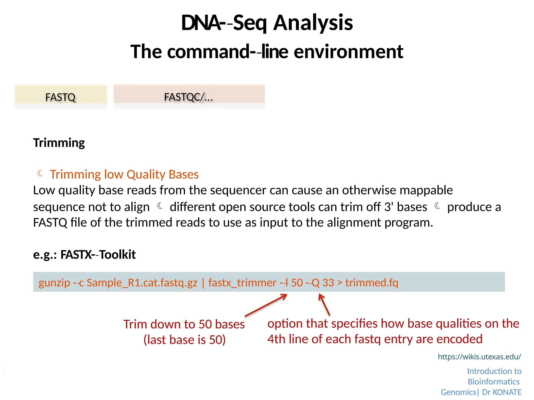
Trimming
Trimming low Quality Bases
Low quality base reads from the sequencer can cause an otherwise mappable
sequence not to align different open source tools can trim off 3' bases produce a
FASTQ file of the trimmed reads to use as input to the alignment program.
e.g.: FASTX-Toolkit
‐
gunzip -c
‐ Sample_R1.cat.fastq.gz | fastx_trimmer -l
‐ 50 -Q
‐ 33 > trimmed.fq
Trim down to 50 bases
(last base is 50)
option that specifies how base qualities on the
4th line of each fastq entry are encoded
https://wikis.utexas.edu/
Introduction to
Bioinformatics
Genomics| Dr KONATE
87.
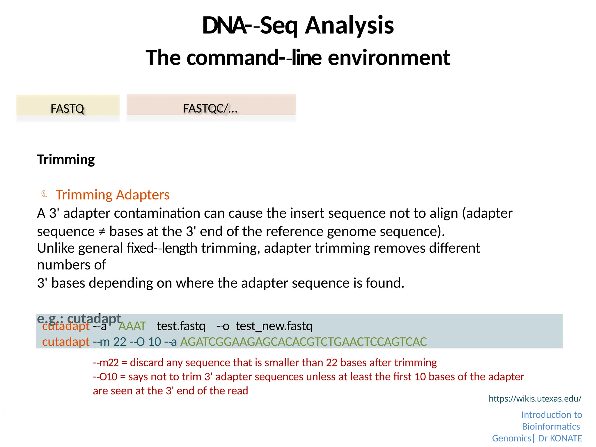
Trimming
Trimming Adapters
A3' adapter contamination can cause the insert sequence not to align (adapter
sequence ≠ bases at the 3' end of the reference genome sequence).
Unlike general fixed-length
‐ trimming, adapter trimming removes different
numbers of
3' bases depending on where the adapter sequence is found.
e.g.: cutadapt
FASTQ FASTQC/…
https://wikis.utexas.edu/
Introduction to
Bioinformatics
Genomics| Dr KONATE
DNA-Seq
‐ Analysis
The command-line
‐ environment
cutadapt -a
‐ AAAT test.fastq -o
‐ test_new.fastq
cutadapt -m
‐ 22 -O
‐ 10 -a
‐ AGATCGGAAGAGCACACGTCTGAACTCCAGTCAC
-m22
‐ = discard any sequence that is smaller than 22 bases after trimming
-O10
‐ = says not to trim 3' adapter sequences unless at least the first 10 bases of the adapter
are seen at the 3' end of the read
88.
DNA-Seq
‐ Analysis
The command-line
‐environment
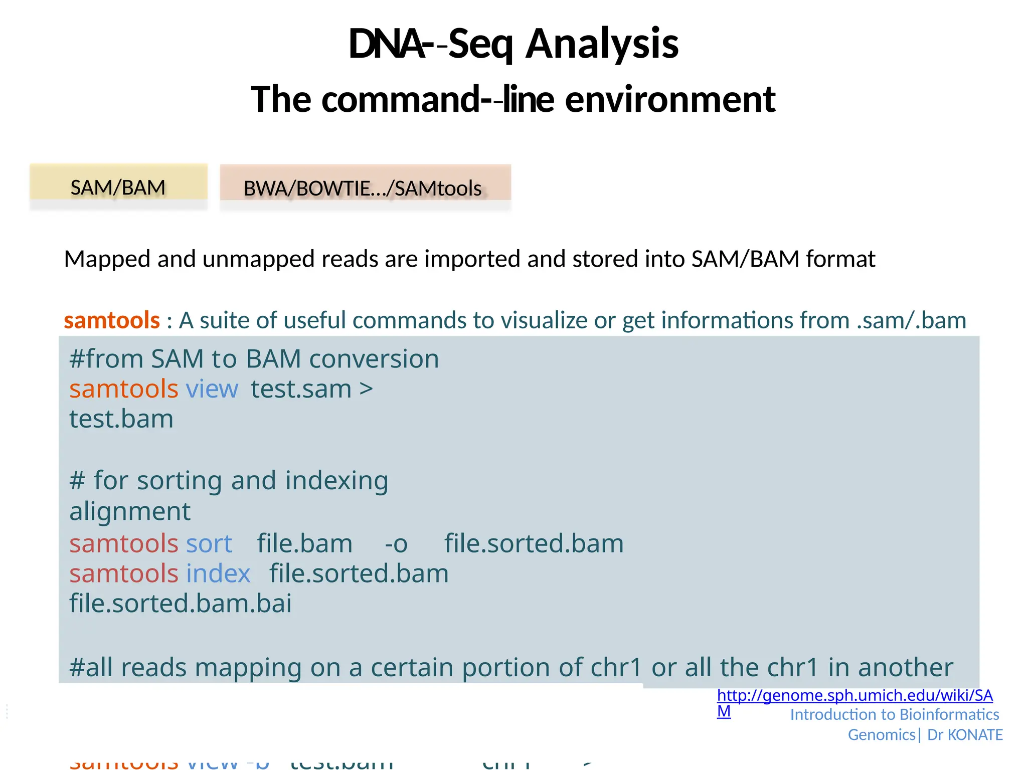
SAM/BAM BWA/BOWTIE…/SAMtools
http://genome.sph.umich.edu/wiki/SA
M
Mapped and unmapped reads are imported and stored into SAM/BAM format
samtools : A suite of useful commands to visualize or get informations from .sam/.bam
#from SAM to BAM conversion
samtools view test.sam >
test.bam
# for sorting and indexing
alignment
samtools sort file.bam -o file.sorted.bam
samtools index file.sorted.bam
file.sorted.bam.bai
#all reads mapping on a certain portion of chr1 or all the chr1 in another
bam samtools index test.bam
samtools view test.bam chr1:200000-500000
samtools view -b test.bam chr1 >
Introduction to Bioinformatics
Genomics| Dr KONATE
89.
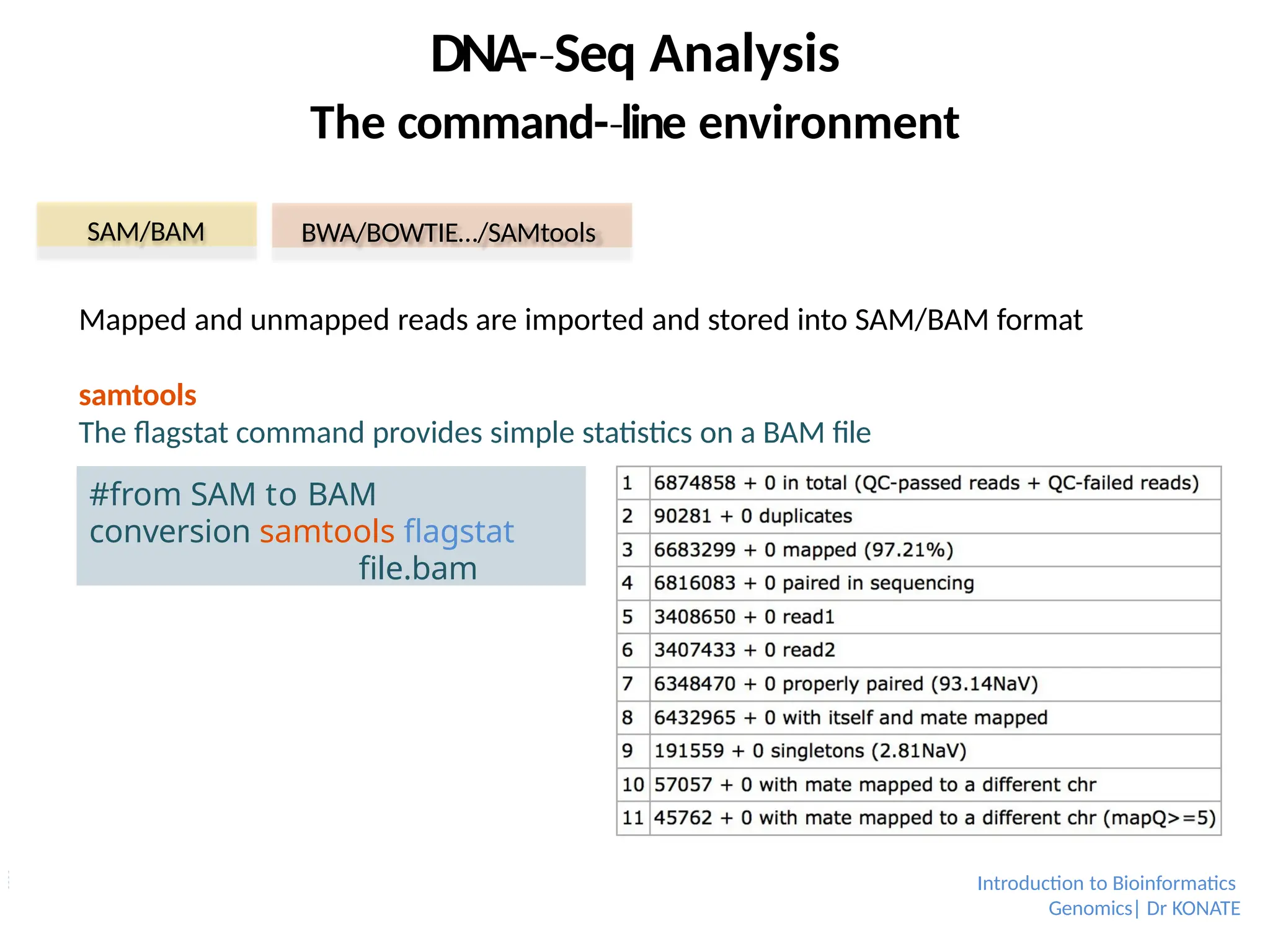
Mapped and unmappedreads are imported and stored into SAM/BAM format
samtools
The flagstat command provides simple statistics on a BAM file
DNA-Seq
‐ Analysis
The command-line
‐ environment
SAM/BAM BWA/BOWTIE…/SAMtools
#from SAM to BAM
conversion samtools flagstat
file.bam
Introduction to Bioinformatics
Genomics| Dr KONATE
90.
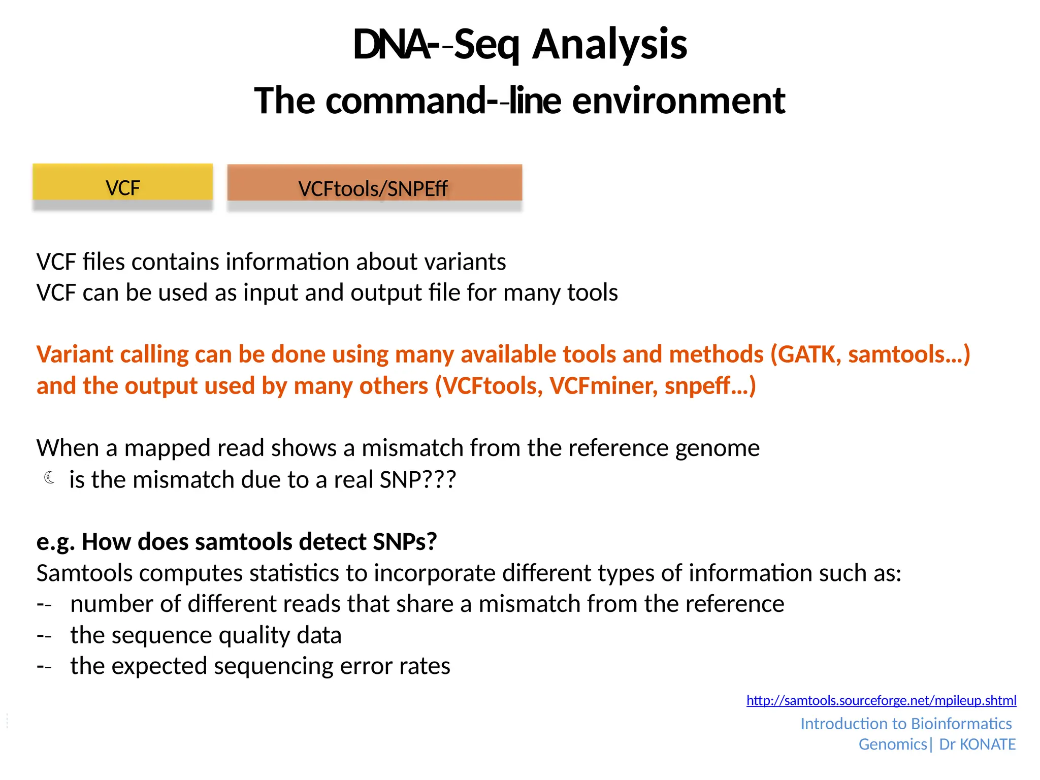
VCF files containsinformation about variants
VCF can be used as input and output file for many tools
Variant calling can be done using many available tools and methods (GATK, samtools…)
and the output used by many others (VCFtools, VCFminer, snpeff…)
When a mapped read shows a mismatch from the reference genome
is the mismatch due to a real SNP???
e.g. How does samtools detect SNPs?
Samtools computes statistics to incorporate different types of information such as:
-
‐ number of different reads that share a mismatch from the reference
-
‐ the sequence quality data
-
‐ the expected sequencing error rates
DNA-Seq
‐ Analysis
The command-line
‐ environment
VCF VCFtools/SNPEff
http://samtools.sourceforge.net/mpileup.shtml
Introduction to Bioinformatics
Genomics| Dr KONATE
91.
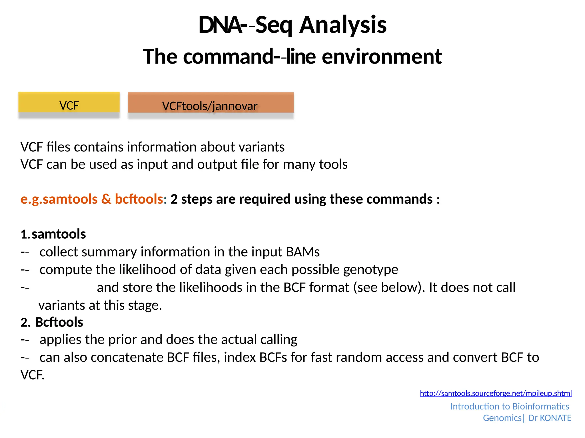
VCF files containsinformation about variants
VCF can be used as input and output file for many tools
e.g.samtools & bcftools: 2 steps are required using these commands :
1.samtools
-
‐ collect summary information in the input BAMs
-
‐ compute the likelihood of data given each possible genotype
-
‐ and store the likelihoods in the BCF format (see below). It does not call
variants at this stage.
2. Bcftools
-
‐ applies the prior and does the actual calling
-
‐ can also concatenate BCF files, index BCFs for fast random access and convert BCF to
VCF.
DNA-Seq
‐ Analysis
The command-line
‐ environment
VCF VCFtools/jannovar
http://samtools.sourceforge.net/mpileup.shtml
Introduction to Bioinformatics
Genomics| Dr KONATE
92.
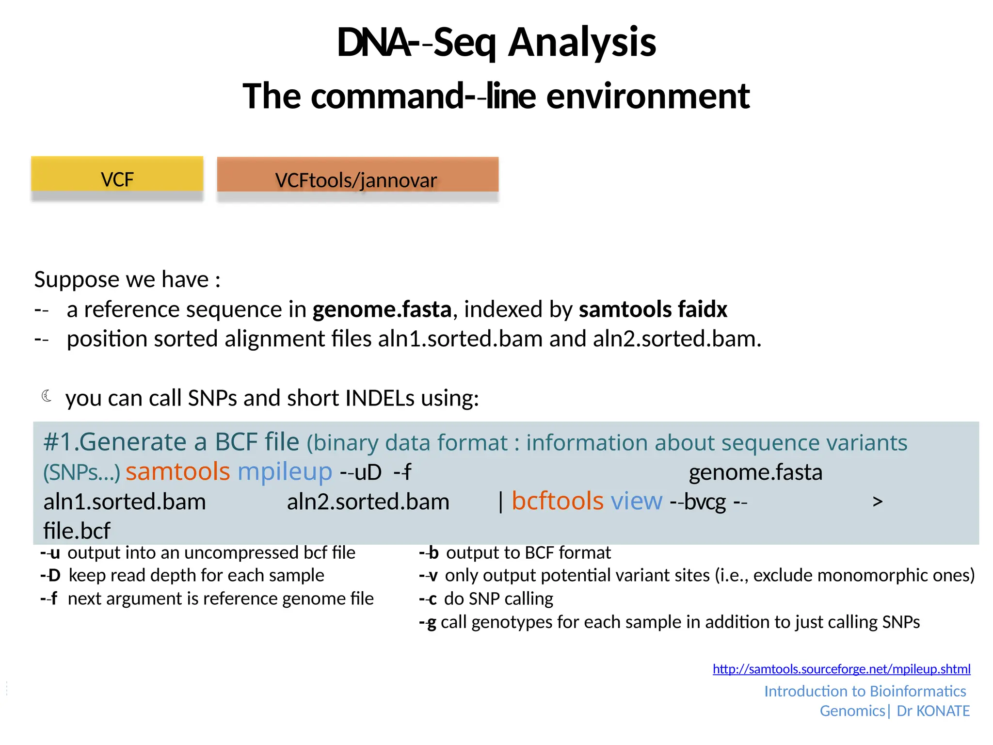
Suppose we have:
-
‐ a reference sequence in genome.fasta, indexed by samtools faidx
-
‐ position sorted alignment files aln1.sorted.bam and aln2.sorted.bam.
you can call SNPs and short INDELs using:
DNA-Seq
‐ Analysis
The command-line
‐ environment
#1.Generate a BCF file (binary data format : information about sequence variants
(SNPs…) samtools mpileup -uD
‐ -f
‐ genome.fasta
aln1.sorted.bam aln2.sorted.bam | bcftools view -bvcg
‐ -
‐ >
file.bcf
VCF
-u
‐ output into an uncompressed bcf file
-D
‐ keep read depth for each sample
-f
‐ next argument is reference genome file
-b
‐ output to BCF format
-v
‐ only output potential variant sites (i.e., exclude monomorphic ones)
-c
‐ do SNP calling
-g
‐ call genotypes for each sample in addition to just calling SNPs
VCFtools/jannovar
http://samtools.sourceforge.net/mpileup.shtml
Introduction to Bioinformatics
Genomics| Dr KONATE
93.
DNA-Seq
‐ Analysis
The command-line
‐environment
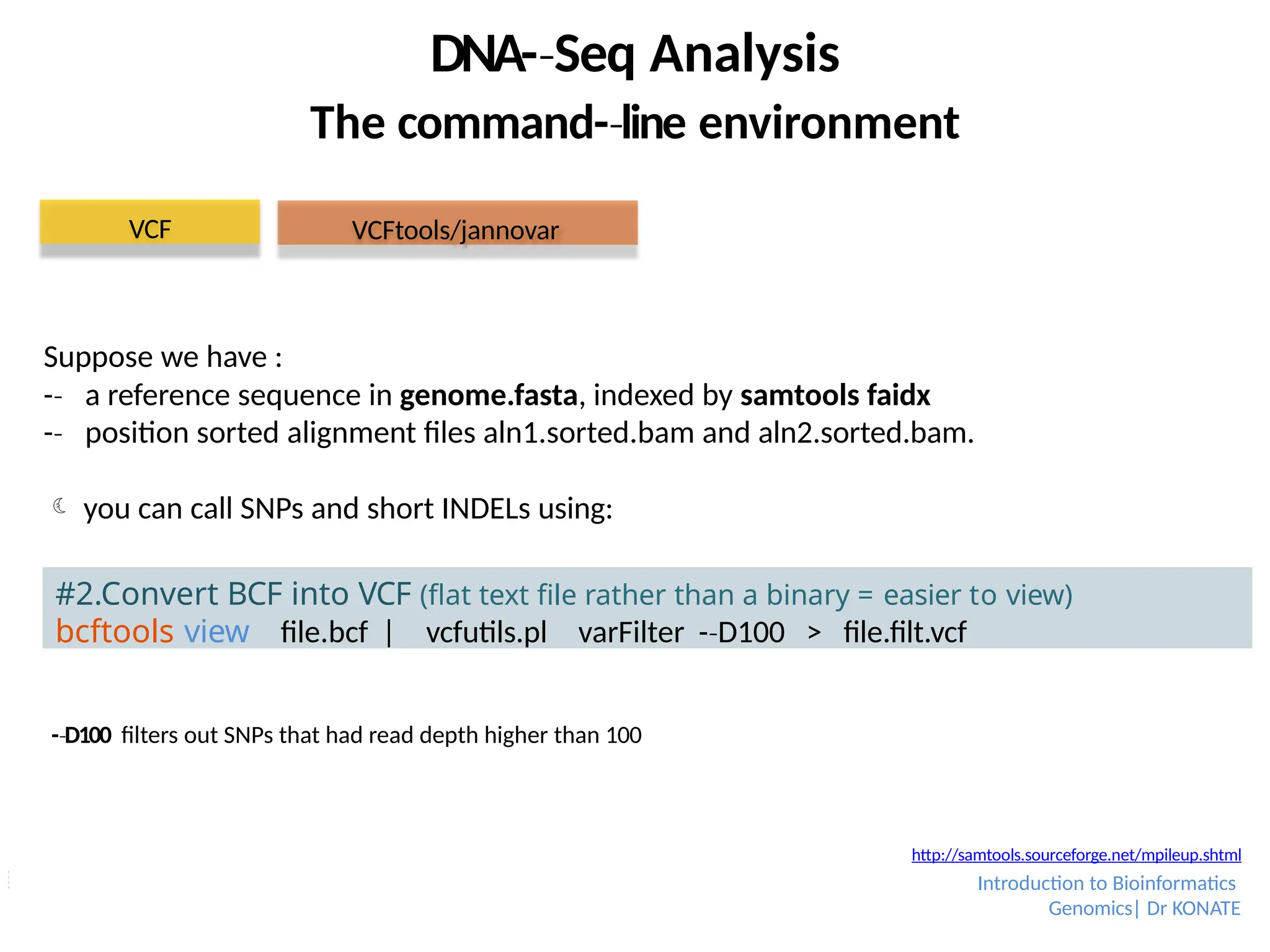
#2.Convert BCF into VCF (flat text file rather than a binary = easier to view)
bcftools view file.bcf | vcfutils.pl varFilter -D100
‐ > file.filt.vcf
VCF
-D100
‐ filters out SNPs that had read depth higher than 100
Suppose we have :
-
‐ a reference sequence in genome.fasta, indexed by samtools faidx
-
‐ position sorted alignment files aln1.sorted.bam and aln2.sorted.bam.
you can call SNPs and short INDELs using:
VCFtools/jannovar
http://samtools.sourceforge.net/mpileup.shtml
Introduction to Bioinformatics
Genomics| Dr KONATE
94.
DNA-Seq
‐ Analysis
The command-line
‐environment
#Download the RefSeq transcript database for the release hg19/GRCh37.
$ java -jar
‐ jannovar-cli-0.23-SNAPSHOT.jar download -d
‐ hg19/refseq
#Annotate the test.vcf file
$ java -jar
‐ jannovar-cli-0.23-SNAPSHOT.jar annotate-vcf -d
‐ hg19_refseq.ser
-i
‐ test.vcf -o
‐ test.jv.vcf
VCF VCFtools/jannovar
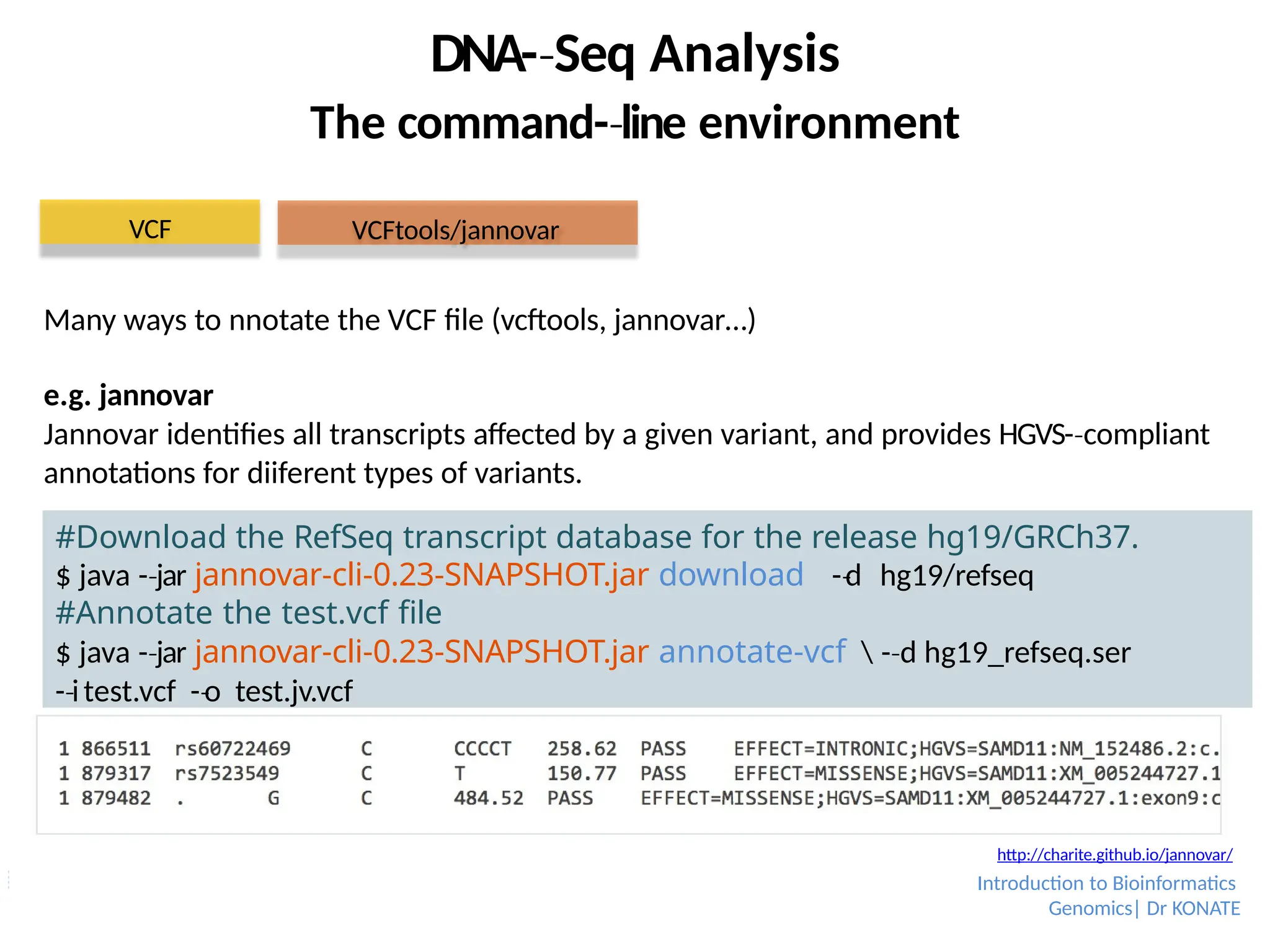
http://charite.github.io/jannovar/
Many ways to nnotate the VCF file (vcftools, jannovar…)
e.g. jannovar
Jannovar identifies all transcripts affected by a given variant, and provides HGVS-compliant
‐
annotations for diiferent types of variants.
Introduction to Bioinformatics
Genomics| Dr KONATE
95.
►all these commandscan be run as part of an analysis pipeline
►all files generated can be parsed using specific tools (samtools…)
►text-based
‐ files generated can be parsed using basic linux commands
►At this stage you should be able to handle easily queries to
parse large files
-
‐ able to search for a particular pattern
-
‐ able to select specific information columns
Introduction to Bioinformatics
Genomics| Dr KONATE
DNA-Seq
‐ Analysis
The command-line
‐ environment
Assignment !
Editor's Notes
#5 Le séquençage de l’ADN est le processus qui consiste à lire les nucléotides présents dans l’ADN, c’est-à-dire à déterminer l’ordre précis des nucléotides au sein d’une molécule d’ADN
Le DNA-Seq désigne aujourd’hui, de manière générale, toute méthode ou technologie de séquençage de nouvelle génération (NGS) utilisée pour déterminer l’ordre des quatre bases (A, T, C, G) dans un brin d’ADN.
#6 En réalité, il existe deux principaux types de technologies de séquençage de l’ADN utilisées aujourd’hui : le séquençage de Sanger et le séquençage de nouvelle génération (NGS).
Chacune de ces technologies a son utilité dans le contexte actuel de l’analyse génétique.
#7 Dans les années 1960-1970, les scientifiques étaient encore en train de comprendre comment les gènes et les génomes fonctionnent, surtout chez les virus à ARN. Le bactériophage MS2 est un virus qui infecte des bactéries (notamment Escherichia coli) et qui possède un génome à ARN simple brin (monocaténaire).
1972 – Min Jou et al. :
Ces chercheurs ont séquencé pour la première fois un gène complet codant pour une protéine (celui de la protéine de la capside) d’un organisme vivant, ici un virus. C’était une étape historique dans la biologie moléculaire, car c’était la première fois que les scientifiques pouvaient lire le code génétique complet d’un gène (nucléotide par nucléotide).
1976 – Fiers et al.
Ce groupe a poursuivi le travail en séquençant l’ensemble du génome du bactériophage MS2, soit 3 569 nucléotides (nt). C’était le tout premier génome complet jamais séquencé dans l’histoire de la science. Cela a permis de comprendre entièrement l’organisation génétique du virus, y compris les gènes, leur ordre, leurs séquences et leurs fonctions.
En 40 ans, les techniques de séquençage sont devenues plus performantes et moins couteuses.
Le développement des technologies de séquençage de nouvelle génération ou NGS (Next Generation Sequencing) durant les 10 dernières années est une révolution technologique sans précédent. Alors que le séquençage d’un seul génome humain aura nécessité 13 ans de collaborations internationales de 1990 à 2003 et 3 milliards de dollars, il est désormais possible, en l’espace de quelques semaines, voire de quelques jours, pour des coûts inférieurs à 1000 €, de séquencer l’intégralité de la région codante des 23 000 gènes humains, l’exome, représentant 34 mil lions de paires de bases de l’ADN. Le séquençage de génomes humains entiers dans un but médical (3 milliards de paires de bases) a déjà été réalisé par quelques équipes aux États-Unis, au Royaume-Uni, aux Pays-Bas et en France. Cette révolution technologique est à l’origine d’une révolution médicale : la médecine de précision ou génomique dont l’objectif est d’optimiser le diagnostic, la prévention et le traitement des maladies humaines en fonction des variations génétiques individuelles
#8 Le Projet Génome Humain (PGH)
Un effort international de 13 ans (de 1990 au 14 avril 2003) visant à séquencer les 3 milliards de "lettres" de l’ADN humain.
Projet d’un coût de 300 millions de dollars, dirigé par le Département de l’Énergie des États-Unis (DoE) et les Instituts Nationaux de la Santé (NIH).
Le Consortium international de séquençage du génome humain (IHGSC) regroupait des chercheurs financés par des fonds publics.
À tout moment, environ 200 laboratoires aux États-Unis soutenaient ces efforts,
et plus de 18 pays du monde entier ont contribué au Projet Génome Humain.
#10 Séquençage hiérarchique par méthode shotgun
Phase "shotgun" :
-Le génome est fragmenté en segments plus larges
-Clonage de ces segments dans des vecteurs
-Séquençage des clones
-Assemblage des séquences shotgun
-Cette méthode repose sur la carte physique du génome humain, établie auparavant.
-Phase de finition :
Comblement des lacunes
Résolution des séquences ambiguës d’ADN
Séquençage shotgun du génome entier
(Celera Genomics)
Le génome est fragmenté aléatoirement en petits morceaux (de taille adaptée au séquençage)
Puis, réassemblage des fragments pour reconstituer le génome.
#11 La qualité du séquençage dépend du nombre moyen de fois que chaque base du génome est « lue » au cours du processus de séquençage.
Pour le Projet Génome Humain (PGH) :
Séquence brouillon : couvre environ 90 % du génome avec une précision d’environ 99,9 %.
Séquence finale : couvre plus de 95 % du génome avec une précision d’environ 99,99 %.
Produire une véritable séquence finale de haute qualité, selon cette définition, est très coûteux et demande beaucoup de travail.
Plusieurs versions de la séquence du génome humain ont été publiées au fil du temps.
#12 Degrés variables de complétion des génomes publiés
Séquençage brouillon (Draft Sequencing)
Phase shotgun ou à haut débit (approche sur l’ensemble du génome ou basée sur des clones)
Assemblage à l’aide d’algorithmes spécifiques (assemblage de tout le génome ou d’un clone individuel)
➔ Précision plus faible que celle d’une séquence finalisée ; certains segments peuvent être manquants, mal ordonnés ou mal orientés.
Finition (Finishing)
Précision dans l’identification des bases, contrôle de qualité, et peu voire aucune lacune
Les segments de séquence sont contigus, ordonnés et reliés les uns aux autres
Aucune ambiguïté ni erreur d’orientation ou d’ordre des segments
Génome complet (Complete Genome)
Un génome représenté par une seule séquence contiguë, sans ambiguïtés
➔ Les séquences disponibles sont finalisées avec une qualité très élevée.
#13 Le Projet Génome Humain (PGH) exigeait que toutes les informations sur les séquences du génome humain soient librement et publiquement accessibles.
Les séquences d’ADN existantes ont été stockées dans des bases de données accessibles à toute personne désireuse de les exploiter et de les analyser.
Des bases de données spécialisées contiennent diverses informations pour les organismes modèles, telles que les séquences de gènes et protéines connues ou hypothétiques (ex. : GenBank, NCBI).
D'autres bases comme Ensembl (http://www.ensembl.org) offrent des données supplémentaires, des annotations, ainsi que des outils puissants pour visualiser et rechercher ces informations.
Des efforts communautaires ont été mis en place pour les organismes non modèles, comme les pathogènes eucaryotes, via des plateformes telles que EuPathDB (http://eupathdb.org/eupathdb/).
Des programmes informatiques ont été développés pour analyser et interpréter ces données.
#14 Le génome humain ne contient qu’environ 20 000 gènes codant pour des protéines, un nombre similaire à celui des nématodes, qui ne possèdent pourtant que 1 000 cellules somatiques.
Les fonctions de ces gènes sont largement orthologues entre les deux espèces (c’est-à-dire qu’elles ont des fonctions équivalentes issues d’un ancêtre commun).
La proportion d’ADN non codant pour des protéines augmente avec la complexité de l’organisme, atteignant plus de 98 % chez l’humain.
➔ ENCODE
➔ GENCODE
#15 ENCODE (https://www.encodeproject.org)
Le projet ENCODE (Encyclopedia of DNA Elements) vise à fournir « une liste des éléments fonctionnels du génome humain », incluant :
des éléments agissant au niveau des protéines et de l’ARN,
ainsi que des éléments régulateurs qui contrôlent les cellules et les conditions dans lesquelles un gène est actif.
« La création d’un tel catalogue est cruciale pour comprendre le fonctionnement du génome. »
GENCODE (http://www.gencodegenes.org)
Le génome humain a fait l’objet d’une annotation manuelle intensive.
Le consortium GENCODE a pour objectif d’identifier toutes les caractéristiques des gènes dans les génomes humain et murin, en combinant :
analyses informatiques,
annotations manuelles,
et validations expérimentales.
#16 Les différences génétiques au niveau des bases individuelles d’un génome (SNPs – Single Nucleotide Polymorphisms) sont de loin le type de variation génétique le plus courant.
Objectif : développer une carte des haplotypes du génome humain
= identifier et cataloguer la majorité des millions de SNPs estimés comme courants dans le génome humain.
Les variants décrits incluent :
leur position dans le génome,
leur répartition entre les individus au sein des populations,
et entre les populations dans différentes régions du monde.
➔ Ce travail est conçu pour fournir des informations permettant de relier les variantes génétiques au risque de maladies spécifiques.
Projet des 1000 Génomes
Ce projet est devenu plus complet et plus fiable à mesure que de nombreux nouveaux variants ont été découverts !
#17 1000 Genomes (www.1000genomes.org/)
Le projet 1000 Genomes a pour objectif d'identifier la majorité des variantes génétiques ayant une fréquence d'au moins 1 %.
Il s'agit d'une ressource libre d'accès sur la variation génétique humaine.
Le jeu de données final inclut les données de 2 504 individus provenant de 26 populations. (séquençage à faible couverture et séquençage de l'exome pour tous).
International Genome Sample Resource (IGSR) assure la pérennité de l’utilisation des données générées par le projet 1000 Genomes.
UK10K (www.uk10k.org/)
Le projet UK10K vise l'identification des variantes génétiques rares à travers l'étude de l'ADN de 4 000 individus et leur comparaison avec les régions codantes des protéines de 6 000 personnes atteintes de maladies documentées.
Il établit des liens entre les variantes génétiques et les maladies rares.
#18 Développement de nouvelles technologies pour augmenter la profondeur du séquençage : les technologies de séquençage de nouvelle génération (NGS)
Depuis leur développement, les technologies NGS ont attiré une attention croissante en raison de leur potentiel considérable d’application en microbiologie diagnostique et en santé publique.
Elles ont révolutionné le processus de séquençage, passant du séquençage Sanger au séquençage à haut débit.
#20 Le séquençage de Sanger est la méthode développée par Frederick Sanger en 1977. Cette technique consiste à copier un brin d’ADN simple à l’aide de bases chimiquement modifiées appelées didéoxynucléotides (ddNTPs).
Lorsque les ddNTPs sont incorporés à l’extrémité 3' de la chaîne en croissance, ils interrompent sélectivement l’élongation de la chaîne à la base A, C, G ou T. Les chaînes ainsi arrêtées sont ensuite séparées par électrophorèse capillaire.
#21 Applied Biosystems (Life Technologies) a fabriqué les séquenceurs capillaires automatisés utilisés à la fois par Celera Genomics et le Projet Génome Humain.
Bien que le séquençage capillaire ait été la première méthode à permettre le séquençage complet d’un génome humain, il s’est révélé trop coûteux et trop long pour une utilisation commerciale à grande échelle !!!
Pour cette raison, le séquençage basé sur la technologie de Sanger a été supplanté par d'autres technologies, telles que le pyroséquençage ou le séquençage SMRT (Single Molecule Real Time)…
#22 Le DNA-Seq est aujourd’hui utilisé comme stratégie de séquençage efficace depuis l’apparition de méthodes rapides de séquençage de l’ADN, qui ont considérablement accéléré la recherche et les découvertes en biologie et en médecine, notamment le séquençage de novo…
Le DNA-Seq peut être utilisé pour déterminer la séquence de gènes individuels, de régions génétiques plus vastes, de chromosomes entiers ou même de génomes complets.
Le DNA-Seq et les autres technologies apparentées dites « seq » permettent d’aborder la complexité du génome, telles que :
le séquençage de l’ADN génomique (genomic DNA-Seq),
le Methyl-Seq,
le ChIP-Seq,
le séquençage de l’exome, etc.
#23 Le séquençage de nouvelle génération (NGS), ou séquençage à haut débit (HT), est un terme générique désignant différentes technologies modernes de séquençage utilisées par diverses plateformes, telles que :
le séquençage Illumina (Solexa),
le séquençage Roche 454,
le séquençage Ion Torrent : Proton / PGM,
etc.
Ces technologies permettent de séquencer l’ADN plus rapidement et à moindre coût que le séquençage de Sanger,
ce qui représente une véritable révolution pour la génomique et la biologie moléculaire.
#25 Principes du séquençage de l’ADN : SBS (Sequencing by Synthesis)
Suivi de l’ajout de nucléotides marqués lors de la copie de la chaîne d’ADN :
Le brin d’ADN matrice est immobilisé.
Des solutions de nucléotides A, C, G et T sont ajoutées et retirées successivement.
Une lumière est émise lorsqu’un nucléotide est complémentaire à la première base non appariée.
Le signal chimioluminescent est détecté pour déterminer la séquence.
#26 La bibliothèque shotgun encadrée par des adaptateurs est amplifiée par PCR sur une cellule de flux (flow cell).
Les deux amorces recouvrent la surface d’un substrat solide.
Les produits d’amplification issus d’un même fragment de la bibliothèque restent localement fixés près de leur point d’origine = cluster.
La PCR produit des clusters clonaux contenant des copies d’un seul brin d’ADN.
#27 Principes du séquençage de l’ADN : Pyroséquençage
L’incorporation de dNTPs par l’ADN polymérase libère du pyrophosphate (PPi).
L’ATP sulfurylase convertit le PPi en ATP en présence d’APS.
L’ATP sert ensuite de substrat pour la conversion de la luciférine en oxyluciférine, catalysée par la luciférase.
Cette conversion génère une lumière dont l’intensité est proportionnelle à la quantité d’ATP, détectée par une caméra.
Les nucléotides non incorporés et l’ATP sont dégradés par l’apyrase, permettant à la réaction de redémarrer avec un autre nucléotide.
#28 La banque d’ADN de type shotgun, flanquée d’adaptateurs, est amplifiée par PCR dans le contexte d’une émulsion eau-dans-huile.
L’amorce de PCR est fixée en 5' sur des billes de taille micrométrique.
Chaque compartiment contenant une bille renferme zéro ou une molécule d’ADN matrice.
Les amplicons PCR sont capturés à la surface de la bille.
Une bille amplifiée de façon clonale contient des produits PCR correspondant à l’amplification d’une seule molécule issue de la banque.
#30 Plateforme Sanger
Séquenceurs capillaires 3730XL (Applied Biosystems®)
Plateforme de séquençage de seconde génération (NGS)
Accès à l’ensemble des plateformes basées sur la technologie Illumina (Miseq, Novaseq, etc.)
Plateforme de séquençage de troisième génération
GridION (Oxford Nanopore Technologies)
Sequel IIe (PacBio)
Plateforme de PCR quantitative et de génotypage
7900 HT (Applied Biosystem)
#31 L'échantillon d'entrée doit être coupé en sections courtes.
Les fragments sont ligaturés à des adaptateurs et hybridés sur la lame à l'aide des adaptateurs.
Les fragments sont séparés en brins simples pour être séquencés.
Les nucléotides sont modifiés de manière à émettre une lumière de couleur différente lorsqu'ils sont excités par un laser.
De plus, ils possèdent un terminateur, de sorte qu'un seul nucléotide est ajouté à la fois.
Le processus de PCR est répété en cycles, puis les images sont analysées.
#33 Comme dans Illumina, l'ADN est fragmenté.
Les adaptateurs sont ajoutés, et les extrémités sont hybridées aux billes.
1 fragment d'ADN = 1 bille.
Les fragments sont amplifiés par PCR à l'aide de primers spécifiques aux adaptateurs. La séquence peut ensuite être déterminée de manière informatique.
Les lectures sont plus longues que celles d'Illumina, avec des longueurs variées.
#35 Le séquençage est effectué avec une ligase, plutôt qu'une polymérase.
Chaque cycle de séquençage introduit une population partiellement dégénérée d'octamères étiquetés fluorescent. La population est structurée de manière à ce que l'étiquette soit corrélée avec l'identité des 2 bases centrales dans l'octamère.
Après la ligature et l'imagerie sur quatre canaux, la portion étiquetée de l'octamère (c'est-à-dire 'zzz') est clivée, laissant une extrémité libre pour un autre cycle de ligature.
#36 Comme dans d'autres types de NGS, l'ADN d'entrée est fragmenté.
Les adaptateurs sont ajoutés et une molécule est placée sur une bille.
L'amplification se fait sur la bille par PCR en émulsion. Chaque bille est placée dans un puits d'une lame.
Le pH est détecté dans chacun des puits, car chaque ion H+ libéré va diminuer le pH. Les variations de pH permettent de déterminer si une base a été ajoutée à la séquence, et combien de bases ont été ajoutées.
Les dNTPs sont ensuite lavés, et le processus est répété en cycles.
#37 **Technologie de séquençage ADN à molécule unique en temps réel (SMRT)
a → Une molécule de polymérase ADN est fixée au fond d'un nanopuits → Le design ZMW garantit qu'un seul nucléotide lié à un colorant peut être excité directement à la fois.
b → Chaque nucléotide phospholinké incorporé restera sur le site actif de l'enzyme pendant quelques millisecondes, ce qui est suffisant pour qu'un signal fluorescent soit enregistré.
NB : Dans d'autres systèmes, l'étiquette fluorescente est attachée à la base dans les nucléotides. Dans la technologie SMRT, l'étiquette fluorescente est attachée à la chaîne de phosphate → Les pentaphosphates étiquetés libérés se diffuseront rapidement.
#38 Représentation schématique du système de séquençage par nanopore.
Protéine supérieure → ssDNA.
2ème protéine
Forme un nanopore dans une membrane.
Contient une molécule adaptatrice qui réduit la vitesse du passage de l'ADN à travers le pore.
Chaque base obstrue le flux à un degré différent.
PromethION…
#40 Vitesse
Le séquençage NGS (Next-Generation Sequencing) est plus rapide que le séquençage Sanger de deux manières :
La réaction chimique peut être combinée avec la détection du signal, tandis que dans le séquençage Sanger, ce sont deux processus distincts.
Une seule lecture peut être effectuée à la fois dans le séquençage Sanger, tandis que le NGS est massivement parallèle.
Coût
Le coût du séquençage du génome humain était de 300 millions de dollars.
Le séquençage d'un génome humain avec Illumina permet d'approcher le coût de 1 000 dollars attendu.
Taille de l'échantillon
Nécessite une quantité de départ de DNA/ARN significativement plus faible.
Précision
Plus de répétitions qu'avec le séquençage Sanger → une couverture plus grande, une plus grande précision et une meilleure fiabilité des séquences (les lectures individuelles sont moins précises pour le NGS).
#44 1, Purification de l’ADN
2. Fragmentation de l'ADN
L'ADN extrait est fragmenté en petits morceaux (généralement entre 150 et 500 pb) à l'aide d'un procédé mécanique (sonication) ou enzymatique. Cette étape crée des fragments d'ADN adaptés à la préparation de la bibliothèque.
3, Réparation des extrémités des fragments d'ADN
Les extrémités des fragments d'ADN sont souvent irrégulières après la fragmentation, et il est nécessaire de les réparer pour qu'elles puissent être ligaturées aux adaptateurs. Ce processus inclut l'ajout de groupements chimiques spécifiques pour rendre les extrémités cohésives et compatibles avec la ligature des adaptateurs.
4. Ajout d'adaptateurs
Des adaptateurs spécifiques sont ligaturés aux extrémités des fragments d'ADN. Ces adaptateurs servent de points d'ancrage pour les étapes suivantes, comme l'amplification PCR et la capture des fragments pendant le séquençage. Ils contiennent souvent des séquences uniques pour le marquage (barcoding) et des séquences nécessaires pour la fixation sur la surface du séquenceur Illumina.
5. Amplification PCR (optionnelle)
Certains protocoles incluent une étape d'amplification PCR pour augmenter la quantité de la bibliothèque avant le séquençage. Cette amplification est réalisée en utilisant des amorces spécifiques qui ciblent les adaptateurs ligaturés sur les fragments. Dans le cas des kits PCR-free, cette étape est omise pour éviter les biais d'amplification.
6. Séquençage
Une fois que la bibliothèque est prête, elle est chargée sur la plateforme de séquençage Illumina. La technologie Illumina permet de lire les fragments d'ADN en parallèle sur une surface de flowcell, produisant des millions de lectures pour une analyse génomique de haute couverture.
#45 kits de préparation de bibliothèques pour le séquençage de l'ADN compatibles avec les plateformes Illumina, qui sont utilisés pour préparer des échantillons d'ADN avant de les séquencer avec des technologies de séquençage de nouvelle génération (NGS), notamment celles proposées par Illumina. Ces kits sont conçus pour différents types d'échantillons et besoins en fonction de la quantité d'ADN, du type d'ADN ciblé (par exemple, ADN mitochondrial ou ADN génomique), et des spécificités de la préparation des bibliothèques.
NEXTflex™ Rapid DNA-Seq Kit : Un kit de préparation de bibliothèques pour le séquençage de l'ADN, qui nécessite entre 1 ng et 1 µg d'ADN en entrée. Ce kit est utilisé pour la préparation rapide de bibliothèques ADN pour le séquençage Illumina.
NEXTflex mtDNA-Seq Kit : Un kit spécifiquement conçu pour la préparation de bibliothèques d'ADN mitochondrial, utile pour les études ciblant l'ADN mitochondrial.
NEXTflex™ DNA Sequencing Kits : Un kit de préparation de bibliothèques pour le séquençage de l'ADN, nécessitant 1 µg d'ADN en entrée.
NEXTflex™ PCR-Free DNA Sequencing Kit : Un kit pour la préparation de bibliothèques d'ADN sans amplification (PCR-free), utilisé lorsque l'échantillon d'ADN est de 0,5 µg à 3 µg. Ce kit permet d'éviter les biais introduits par l'amplification PCR.
NEXTflex™ PCR-Free Barcodes : Des codes-barres (jusqu'à 48) pour être utilisés avec le kit PCR-Free et d'autres protocoles de séquençage de l'ADN.
KAPA HyperPlus Kits : Un kit de préparation de bibliothèques pour des quantités d'ADN en entrée allant de 1 ng à 1 µg. Il permet une préparation efficace avec une large gamme de quantités d'ADN.
KAPA Hyper Prep Kits : Un kit conçu pour préparer des bibliothèques d'ADN à partir de 250 ng d'ADN de tissus formol-fixés et paraffine-embed, avec moins de cycles d'amplification, permettant ainsi de réduire les taux de duplication tout en maintenant une bonne couverture du génome.
Ces kits sont utilisés pour optimiser la préparation des échantillons avant leur séquençage sur des plateformes Illumina, permettant des analyses plus rapides et plus fiables des génomes.
#46 Quantification et évaluation de la bibliothèque
La concentration de la bibliothèque d'ADN est mesurée à l'aide de méthodes comme la spectrophotométrie (ex. Nanodrop), la PCR quantitative, ou les systèmes comme le Qubit pour s'assurer que la bibliothèque est prête pour le séquençage. Des contrôles de qualité supplémentaires, comme l'analyse de la taille des fragments par électrophorèse sur gel ou sur un analyseur de fragments, peuvent être effectués.
#52 Fournis ou conçus sur mesure
La concentration des adaptateurs influence la ligature, ainsi que le transfert des dimères d'adaptateurs et des adaptateurs eux-mêmes.
Efficacité de ligature robuste pour des rapports molaires adaptateur : insert compris entre 10:1 et >200:1.
Rapport d'adaptateurs >200:1 pour les applications à faible quantité d'entrée.
Qualité des adaptateurs
Nettoyage post-ligation.
#53 Sélection de taille 300 – 400 pb ou 350 – 500 pb, après la ligation.
Assure une couverture maximale de la plupart des insertions.
Problème de couverture non uniforme du génome.
Problème de perte de matériau.
Stratégie pour se concentrer sur les longueurs de lecture lors de la préparation de l'échantillon et de la bibliothèque.
#54 Les méthodes de sélection par double immobilisation en phase solide (SPRI) inversée permettent de remodeler la distribution des fragments d'entrée en plages bien définies.
SPRI + Reverse-SPRI.
#55 Amplifie la quantité d'ADN dans la bibliothèque
Enrichit sélectivement les fragments d'ADN avec des molécules d'adaptateur aux deux extrémités.
Nettoyage post-amplification.
#56 Séquençage de l'ADN
Entrée : Bibliothèque construite
Génome complet
Exome complet
Région cible
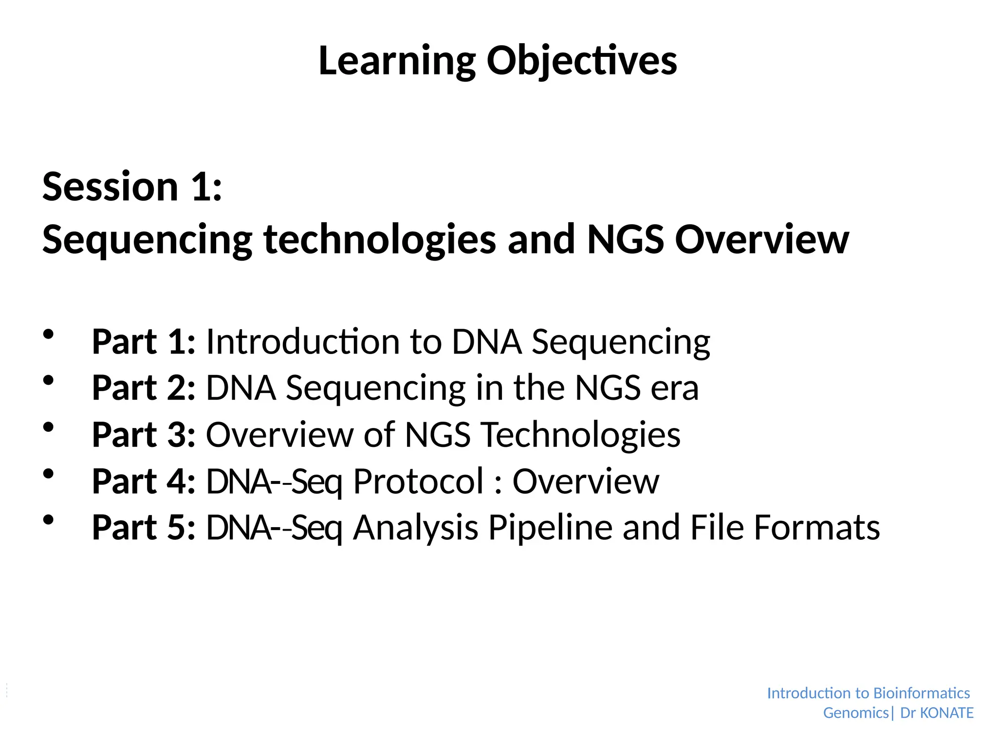
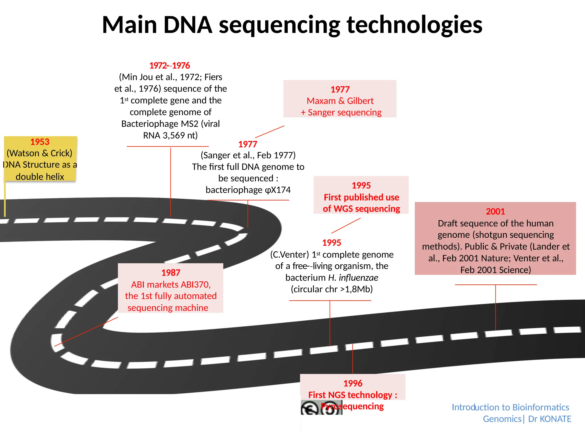
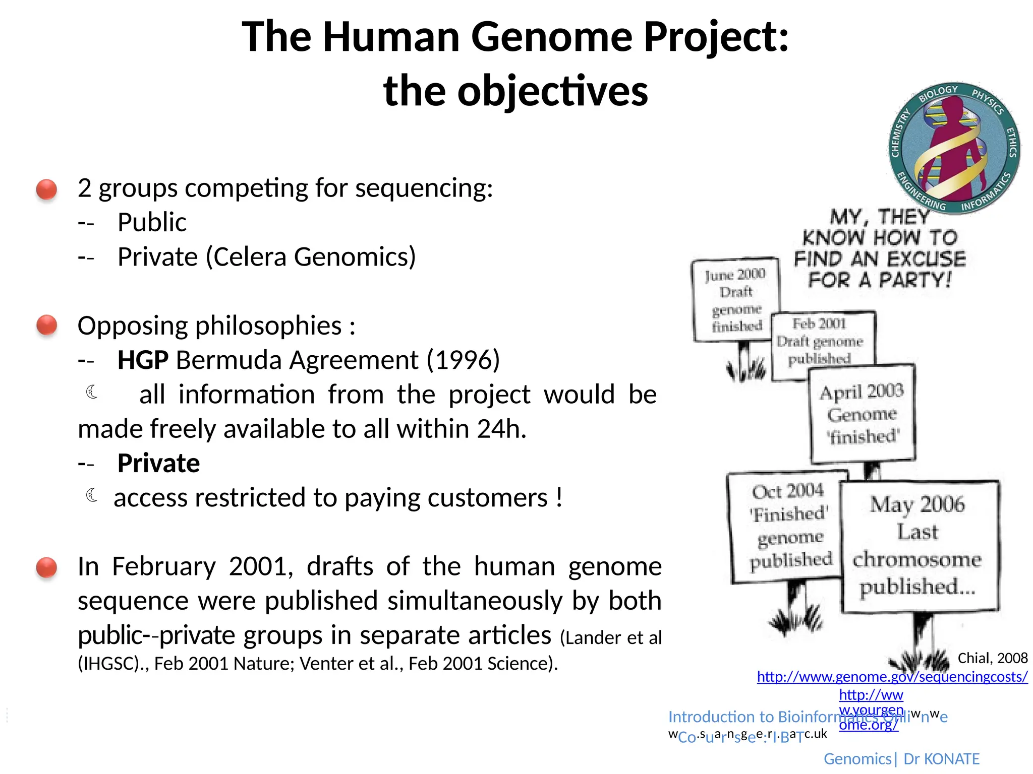
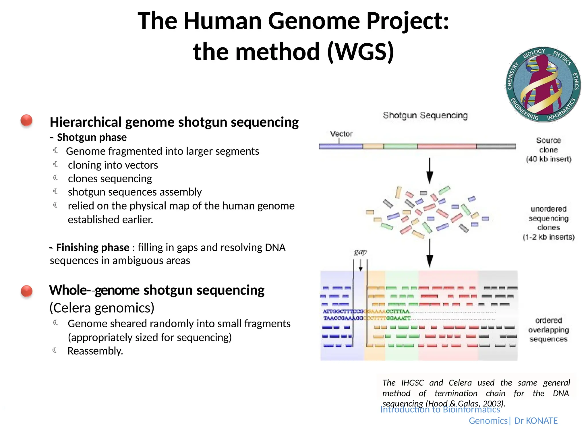
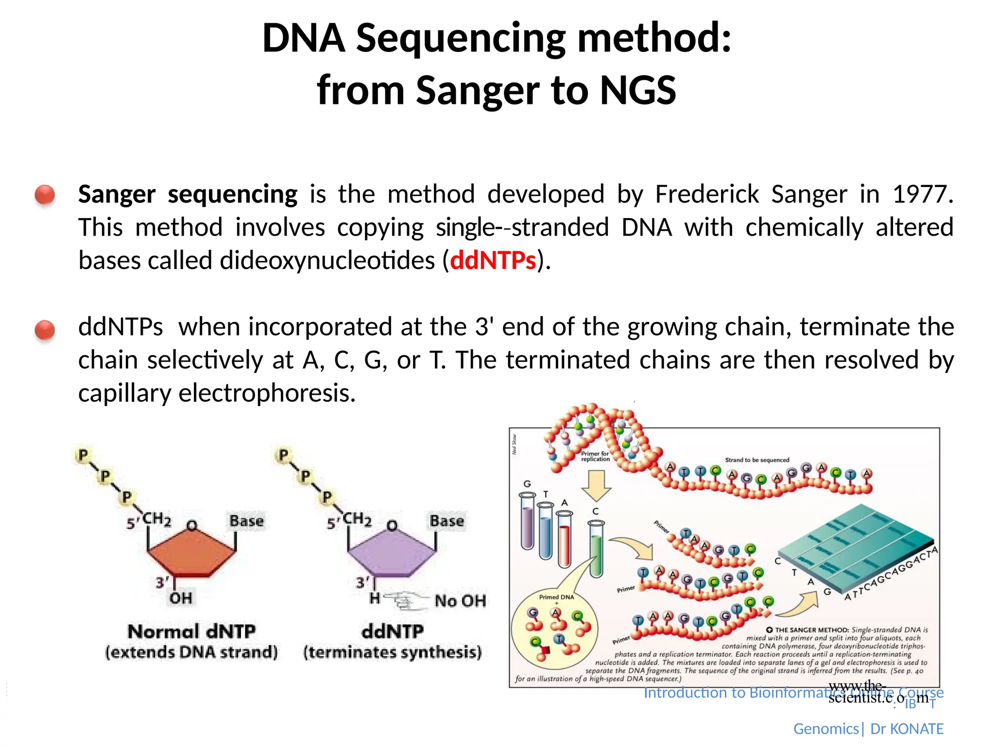
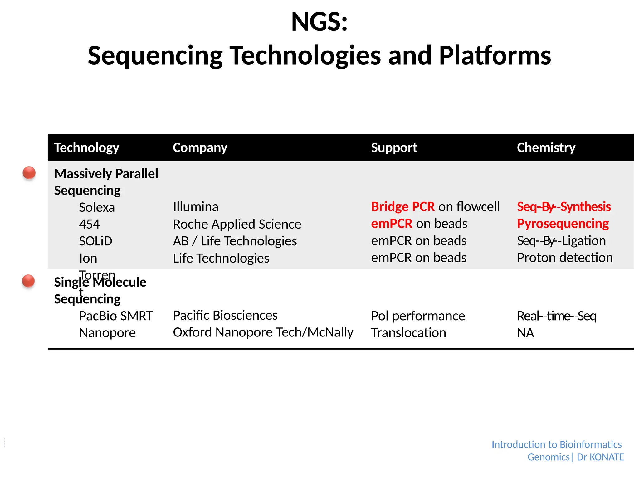
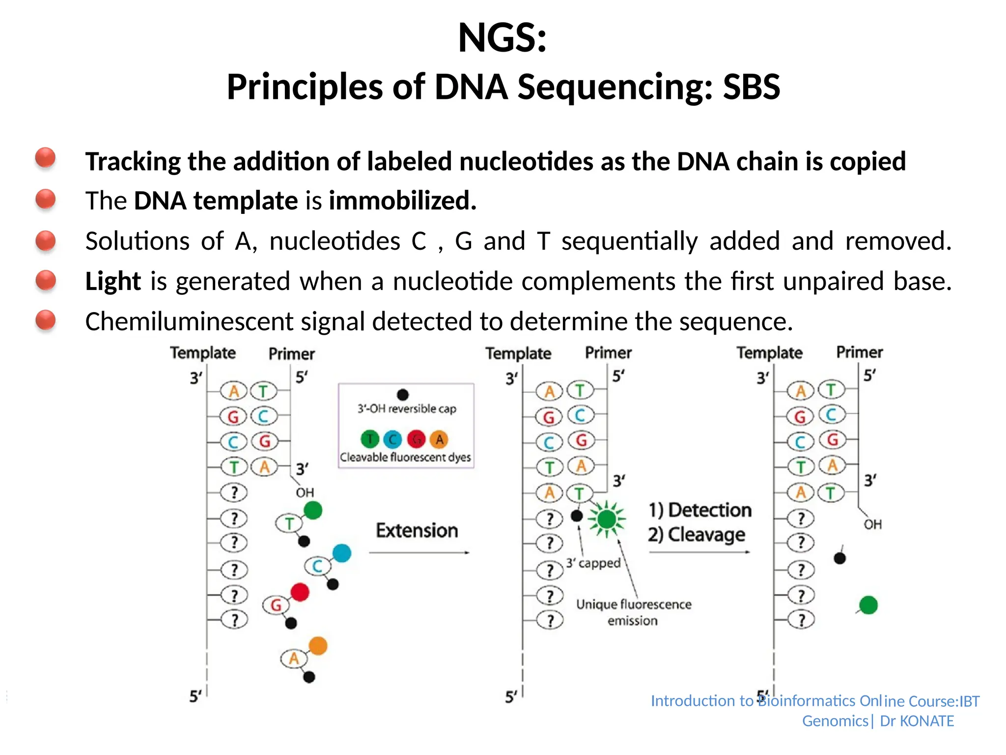
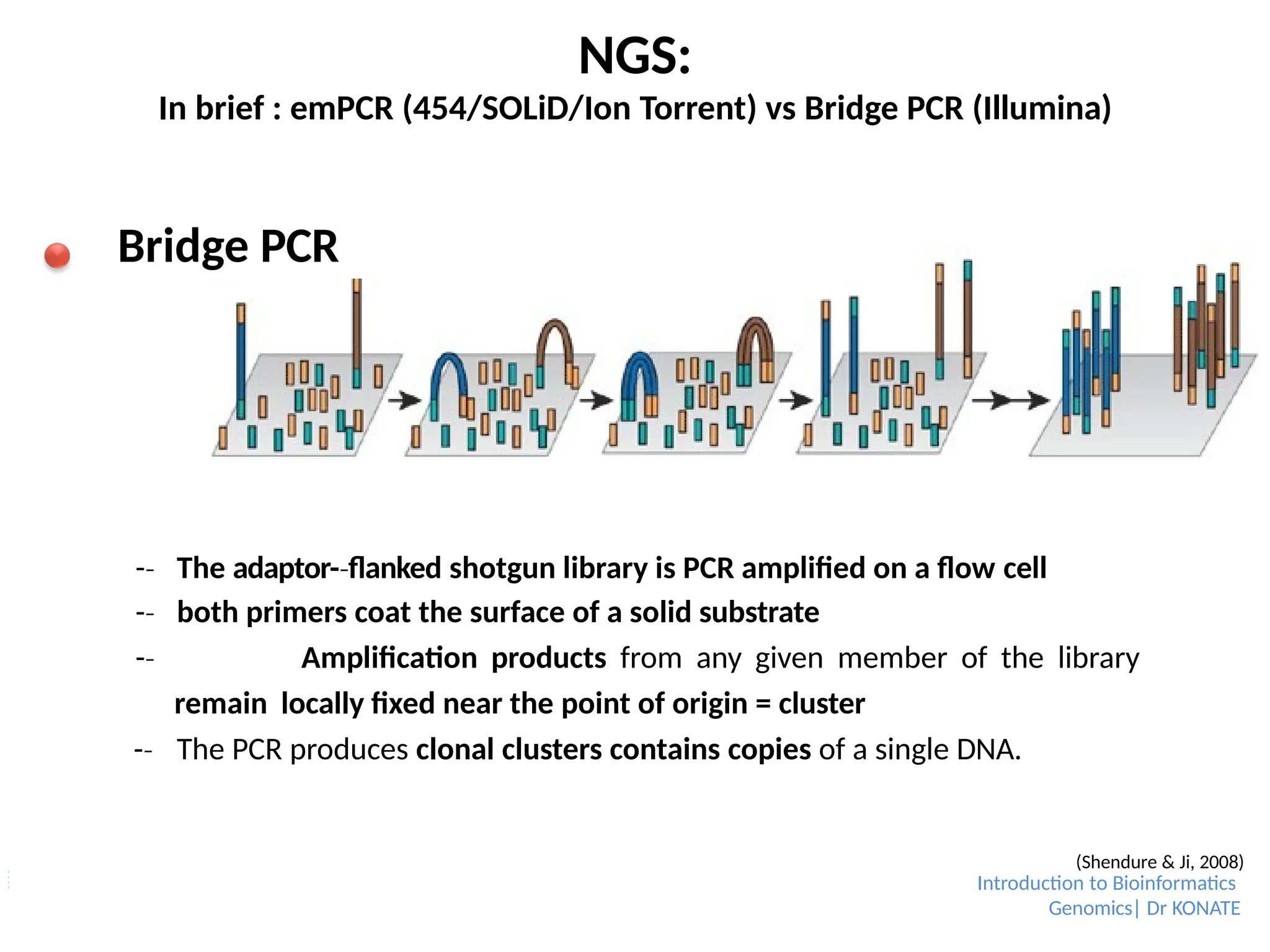
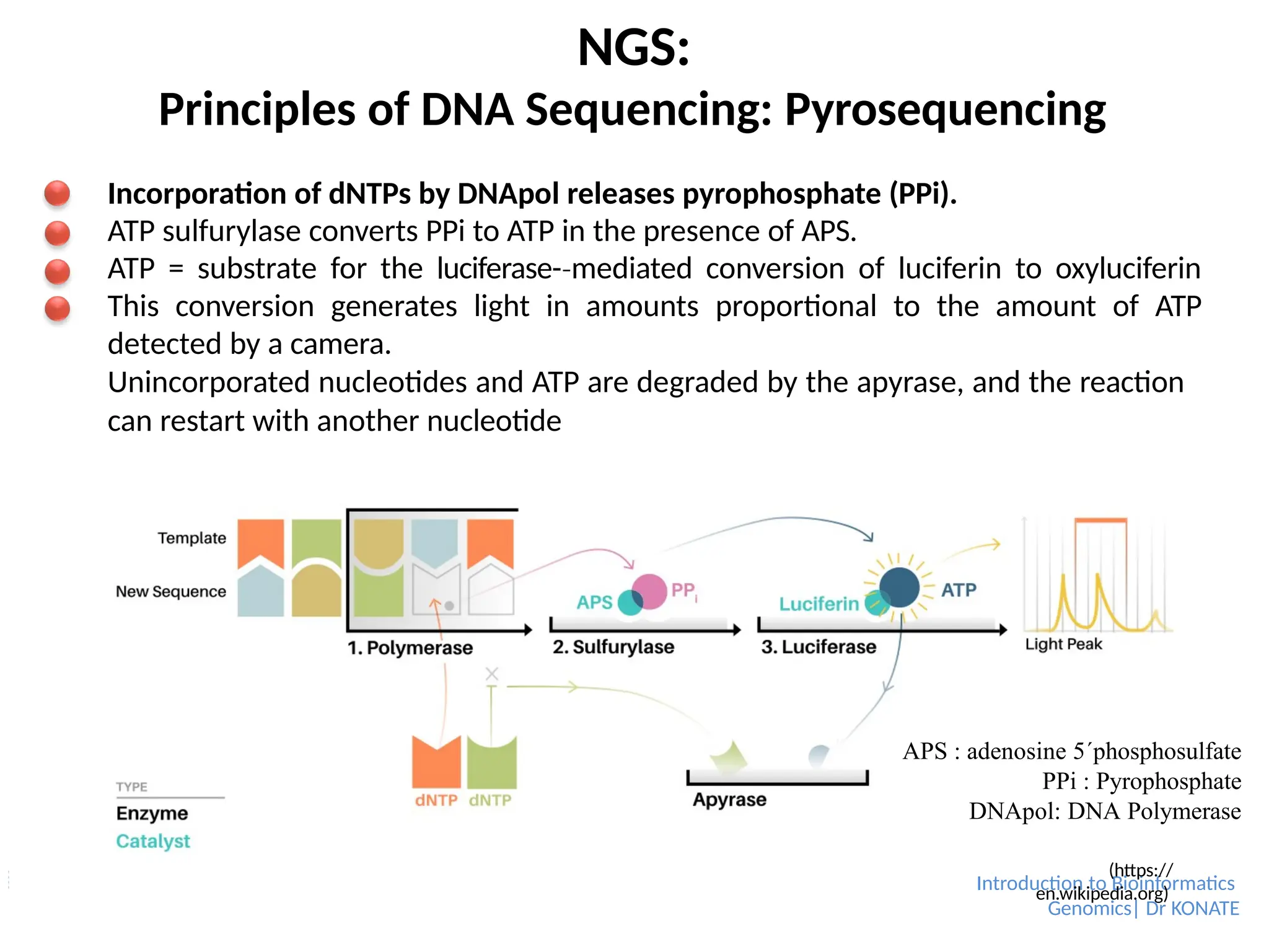
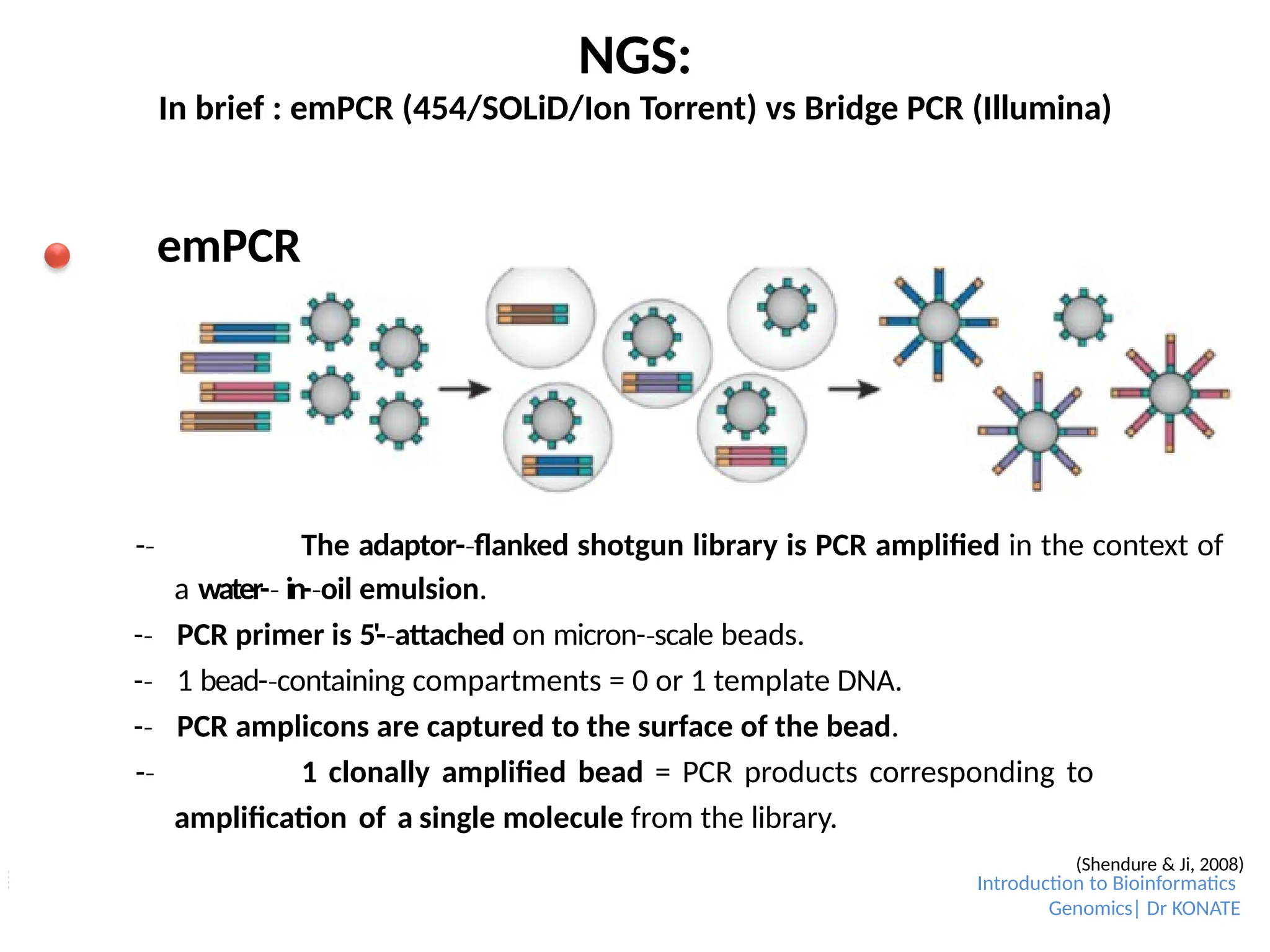
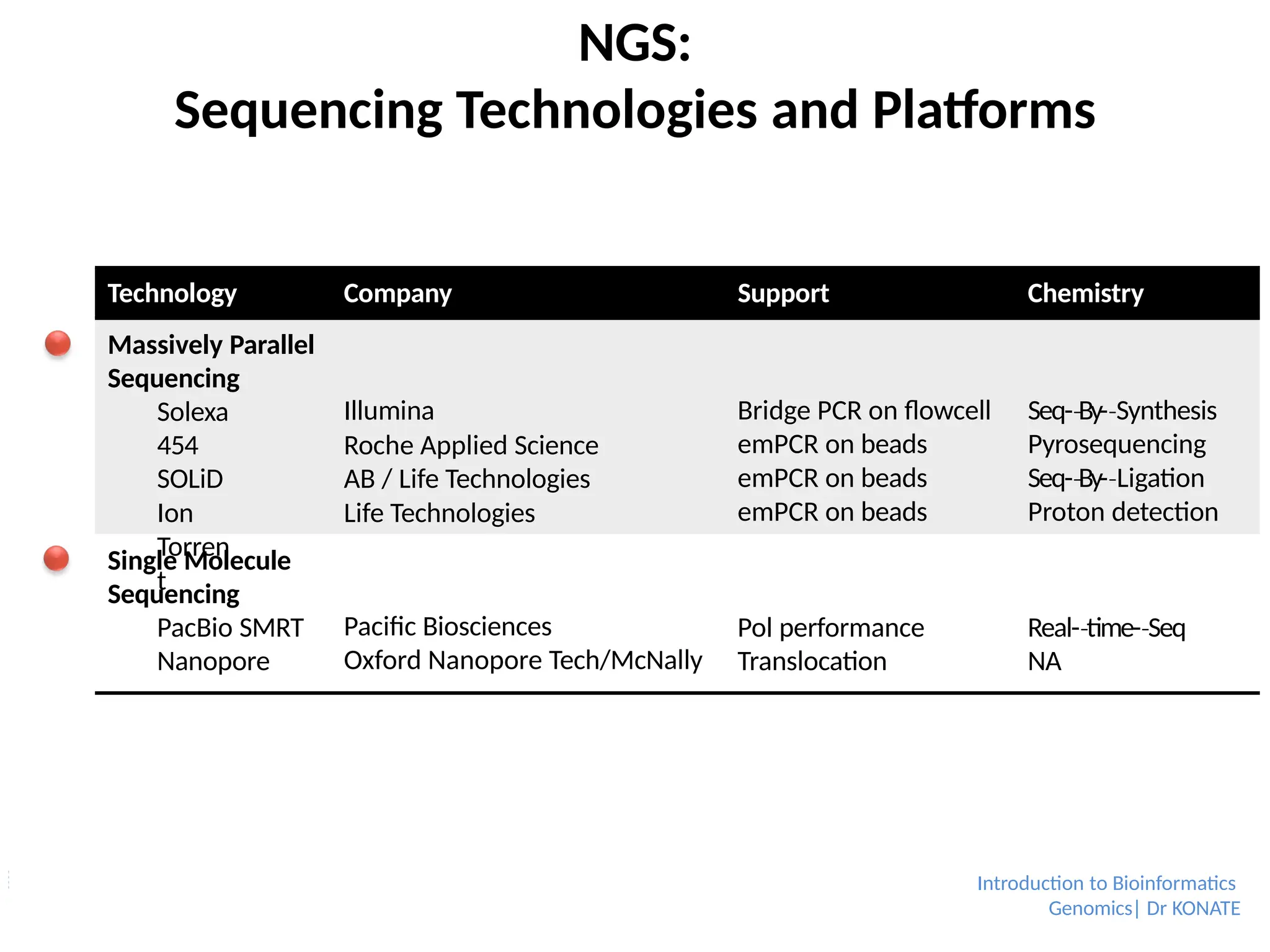
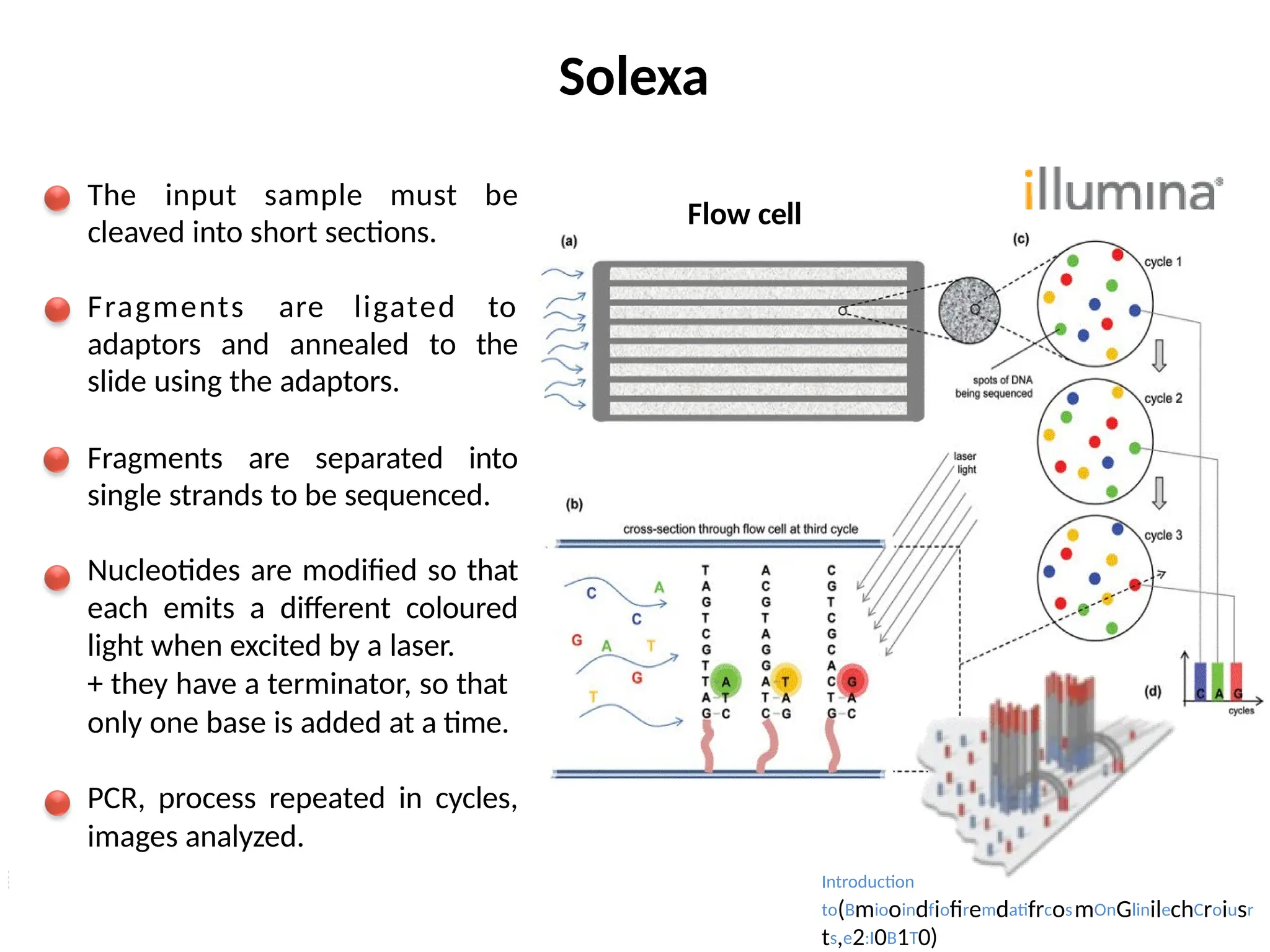
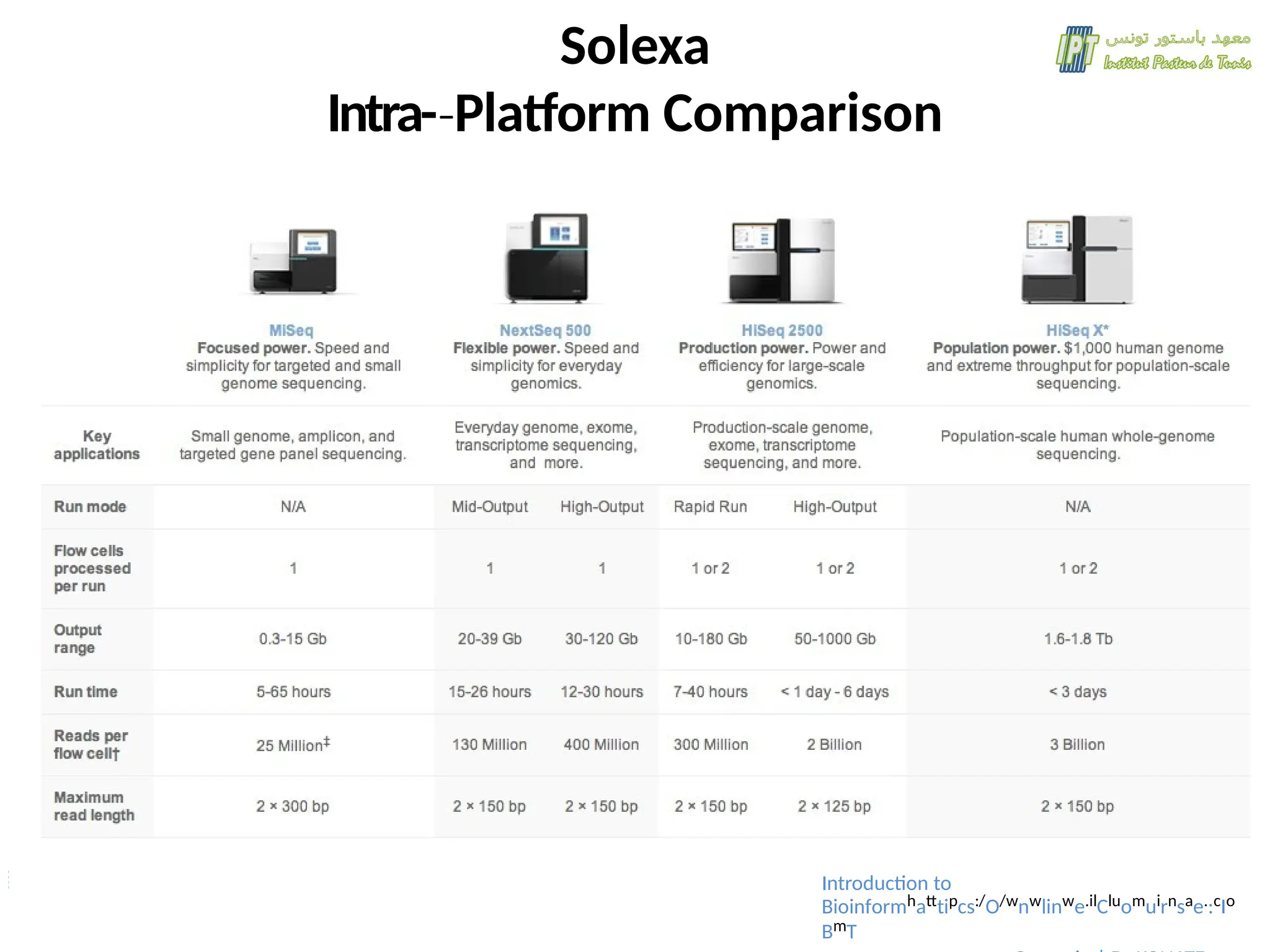
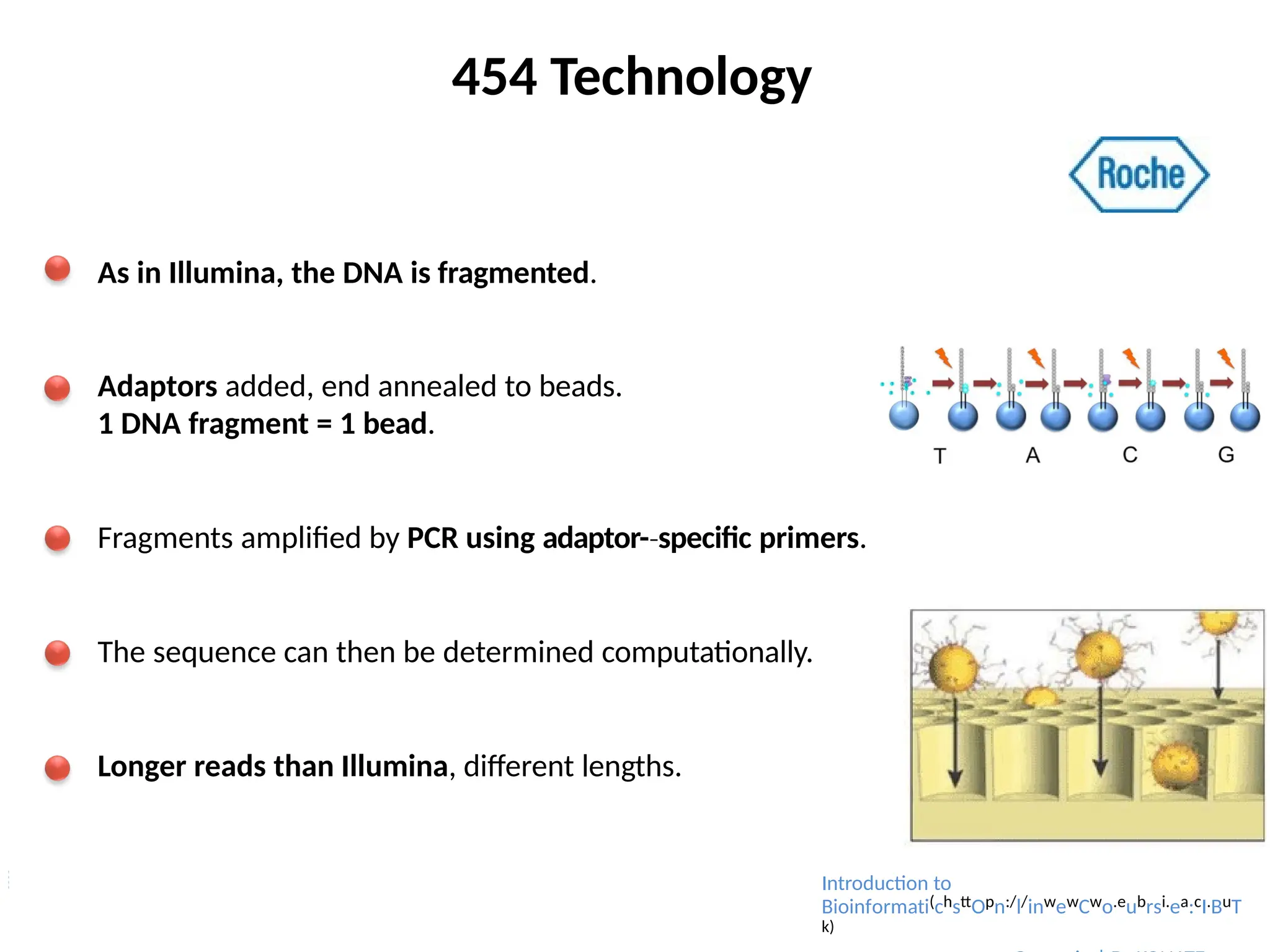
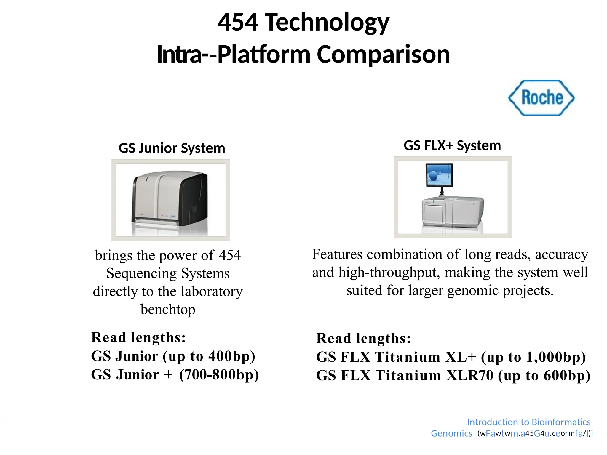
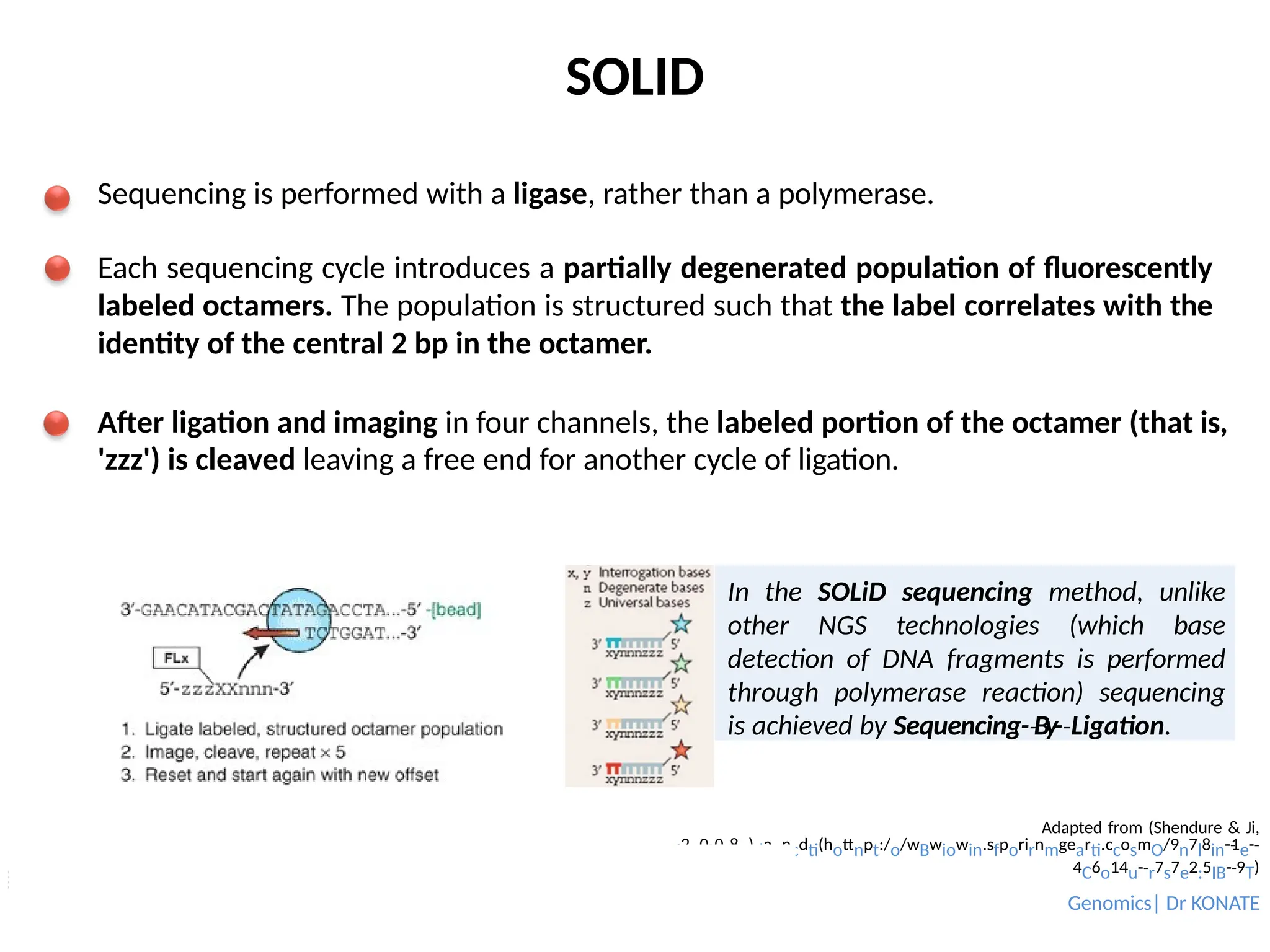
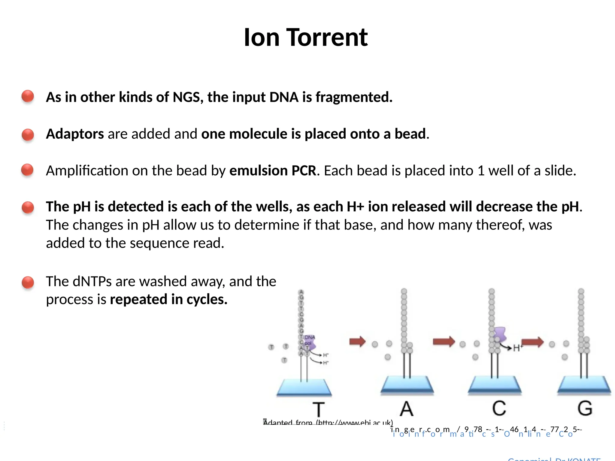
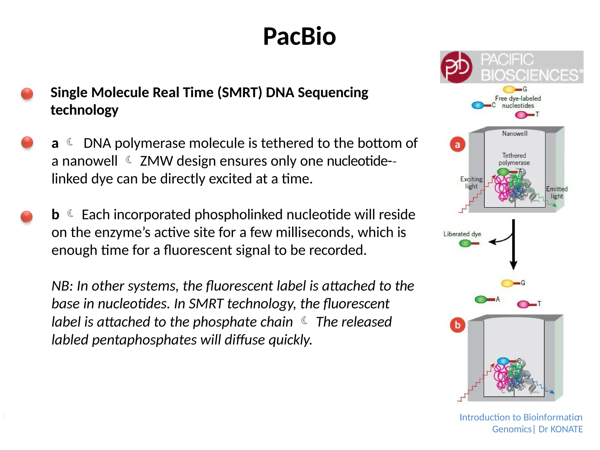
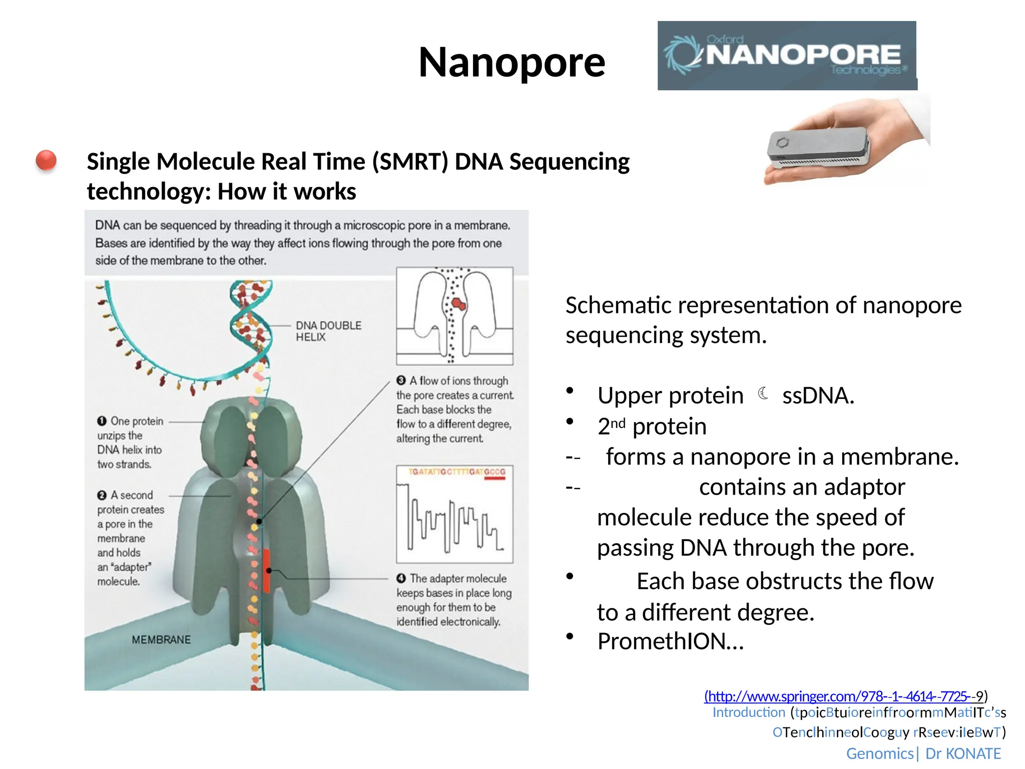
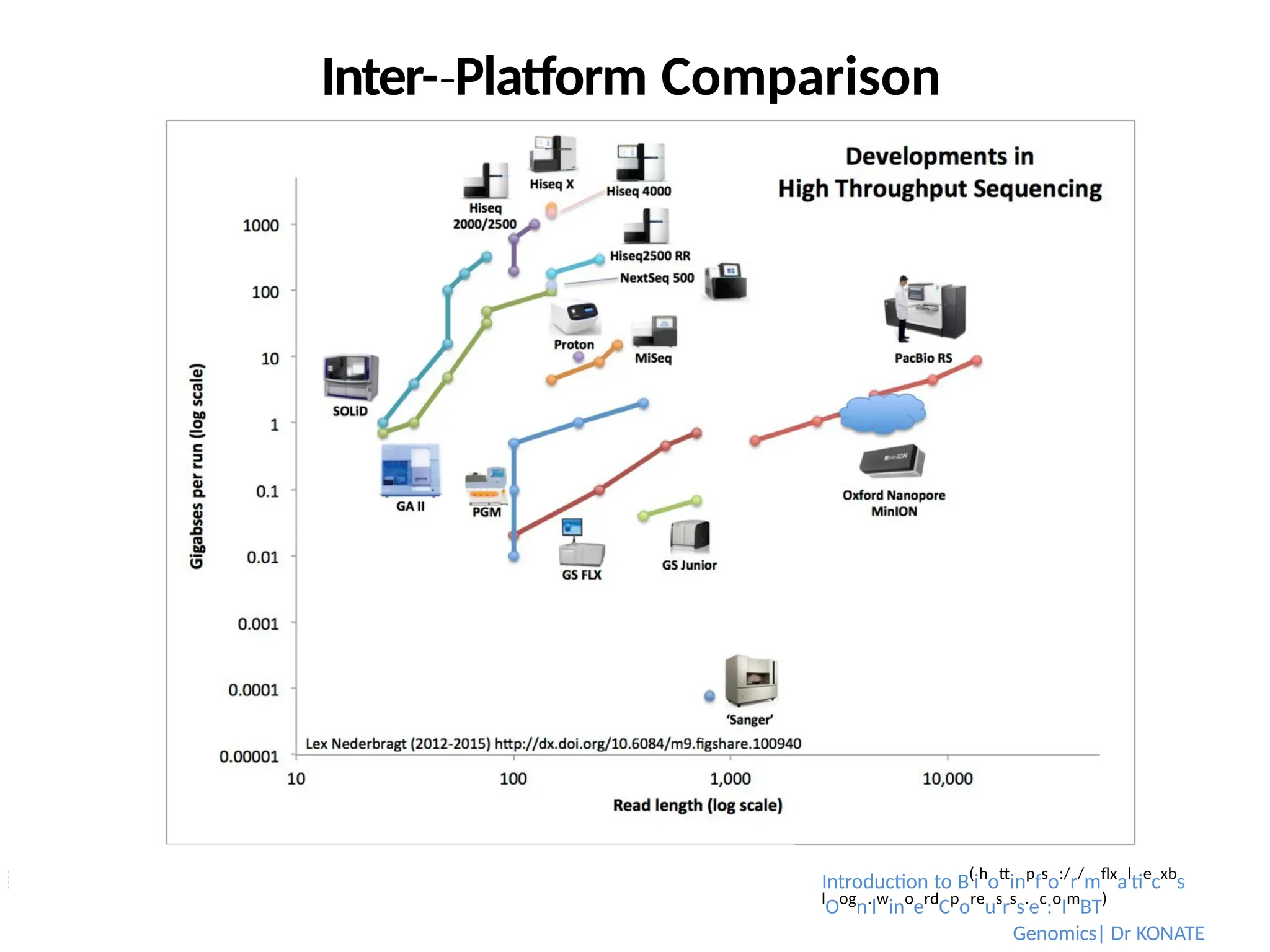
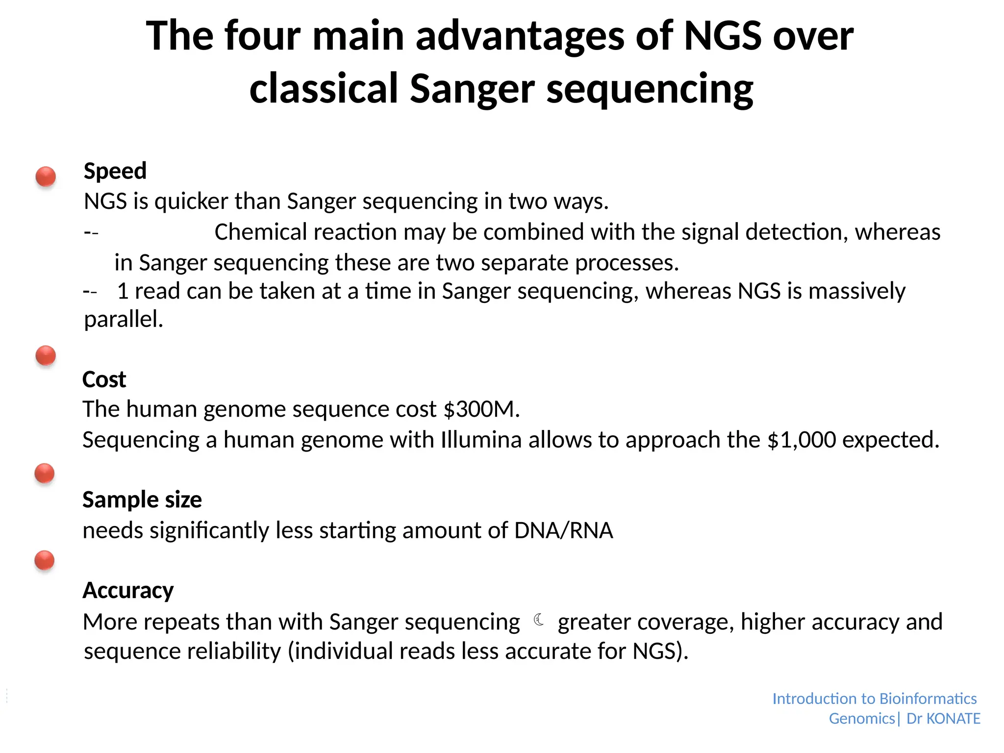
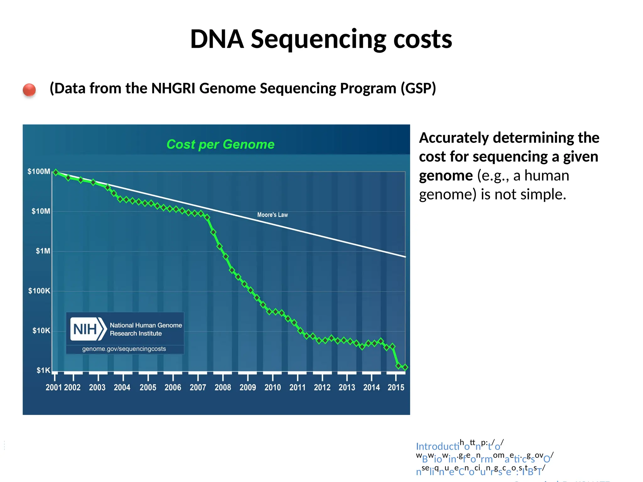
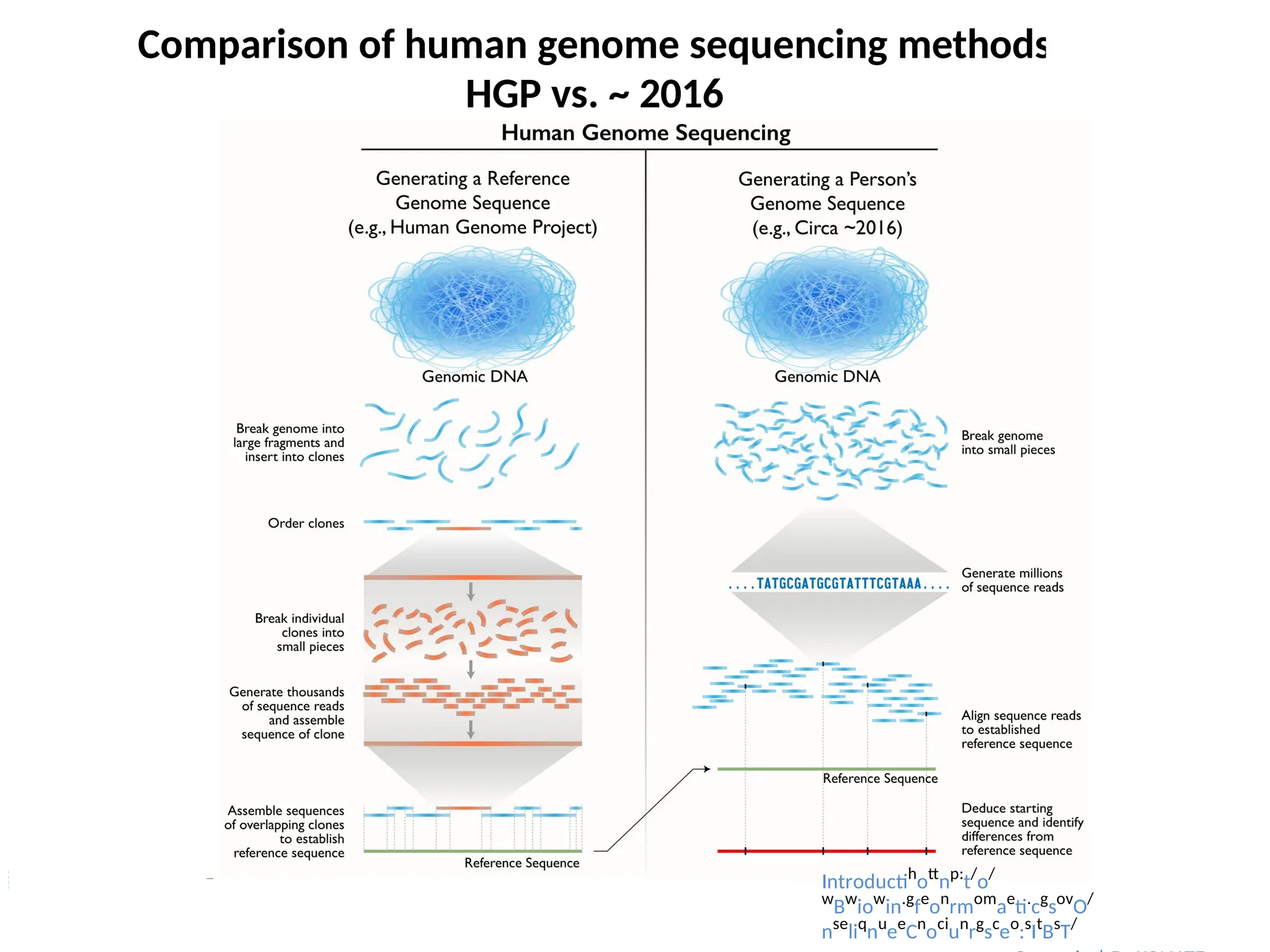
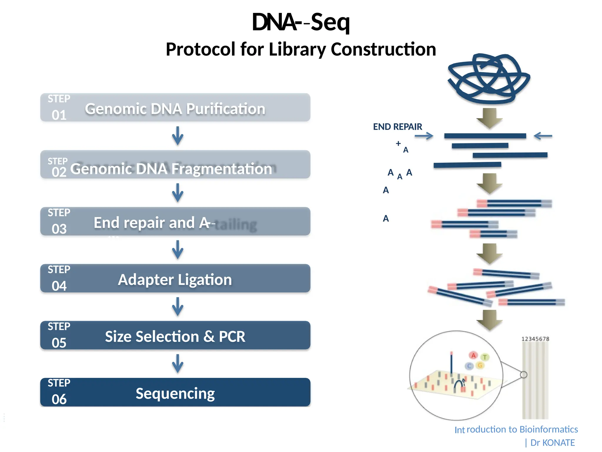
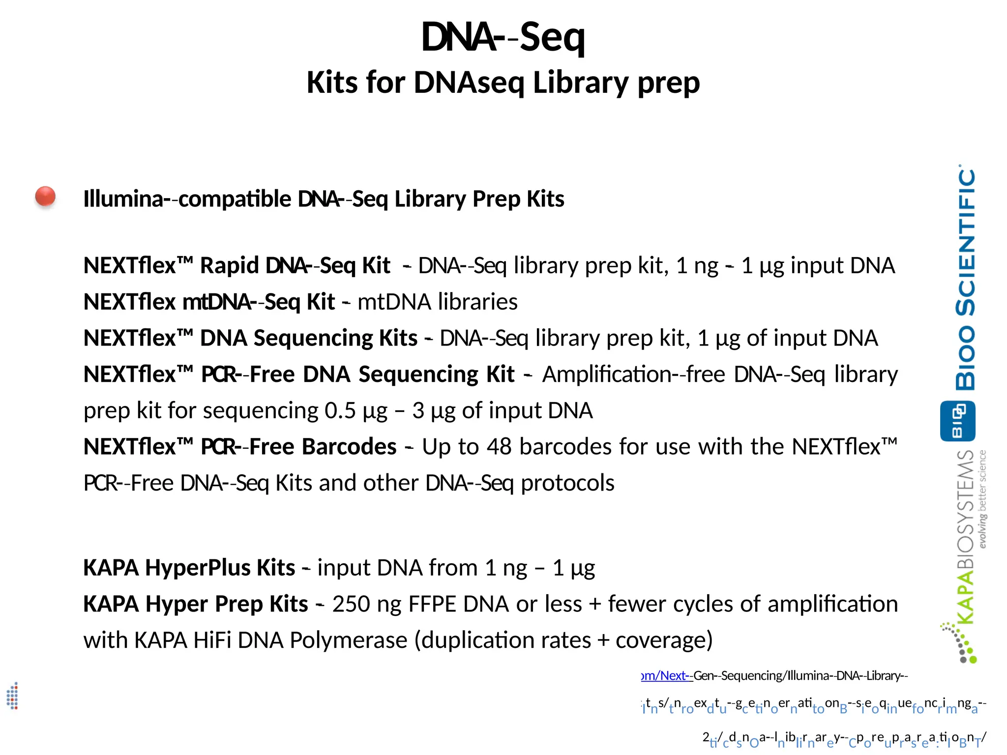
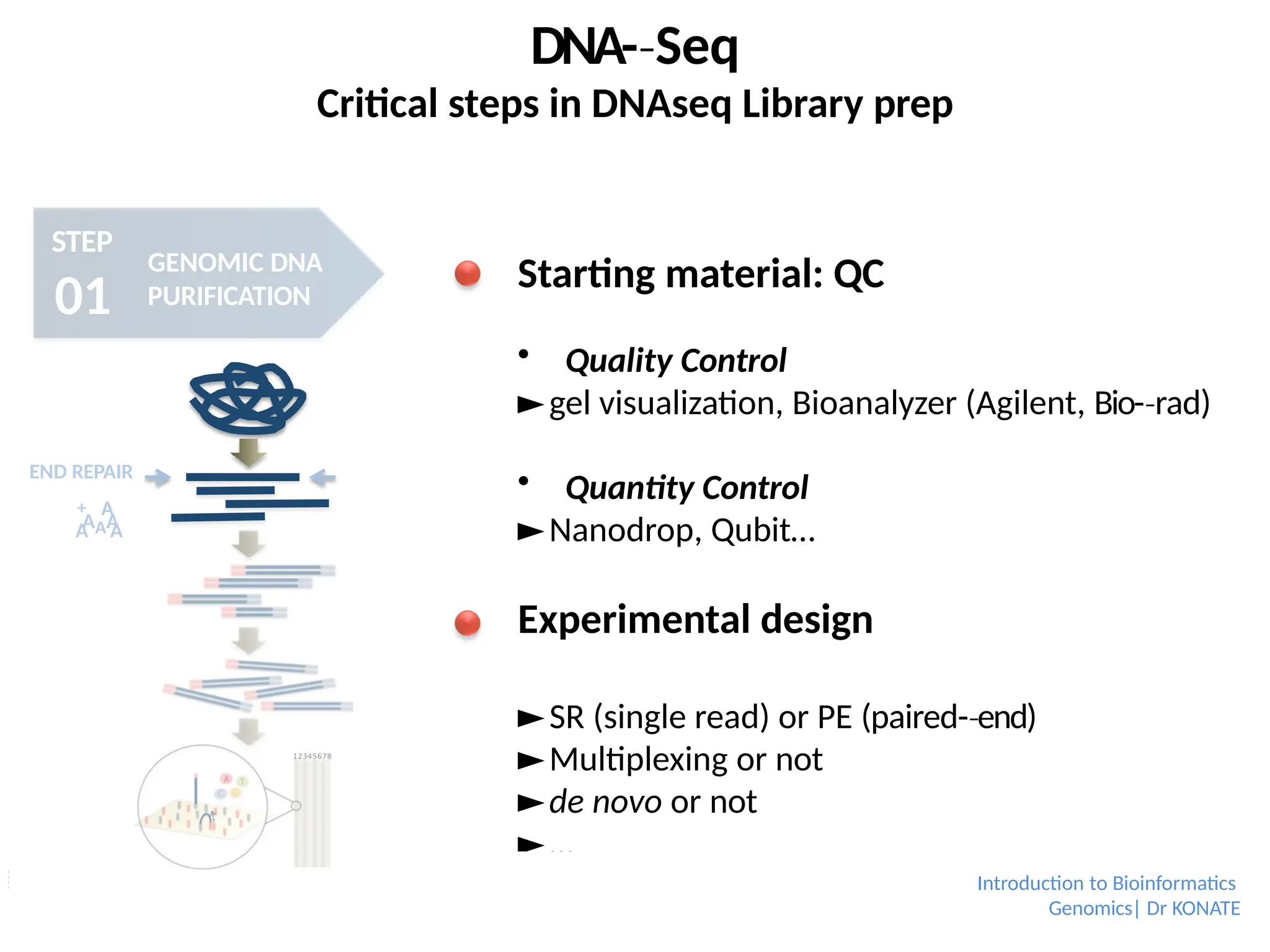
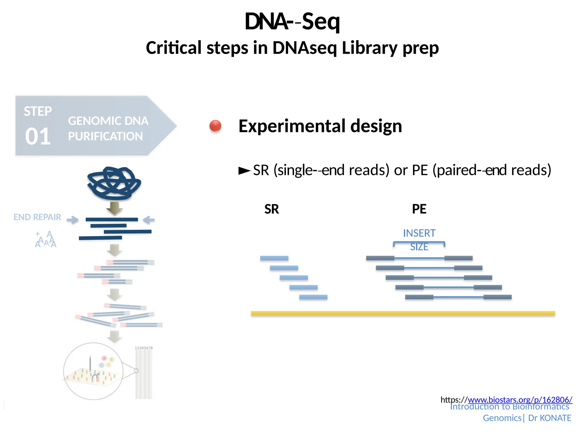
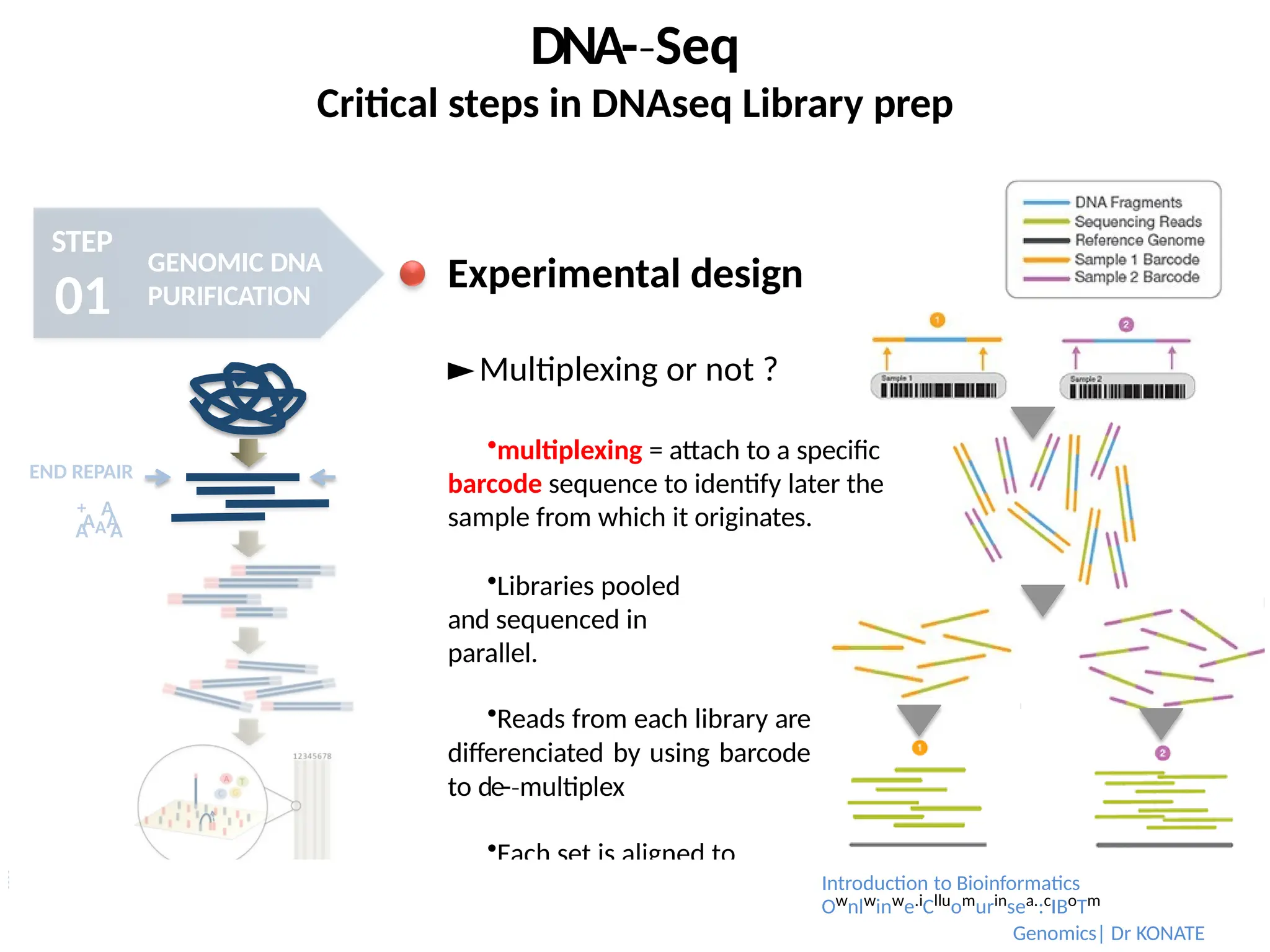
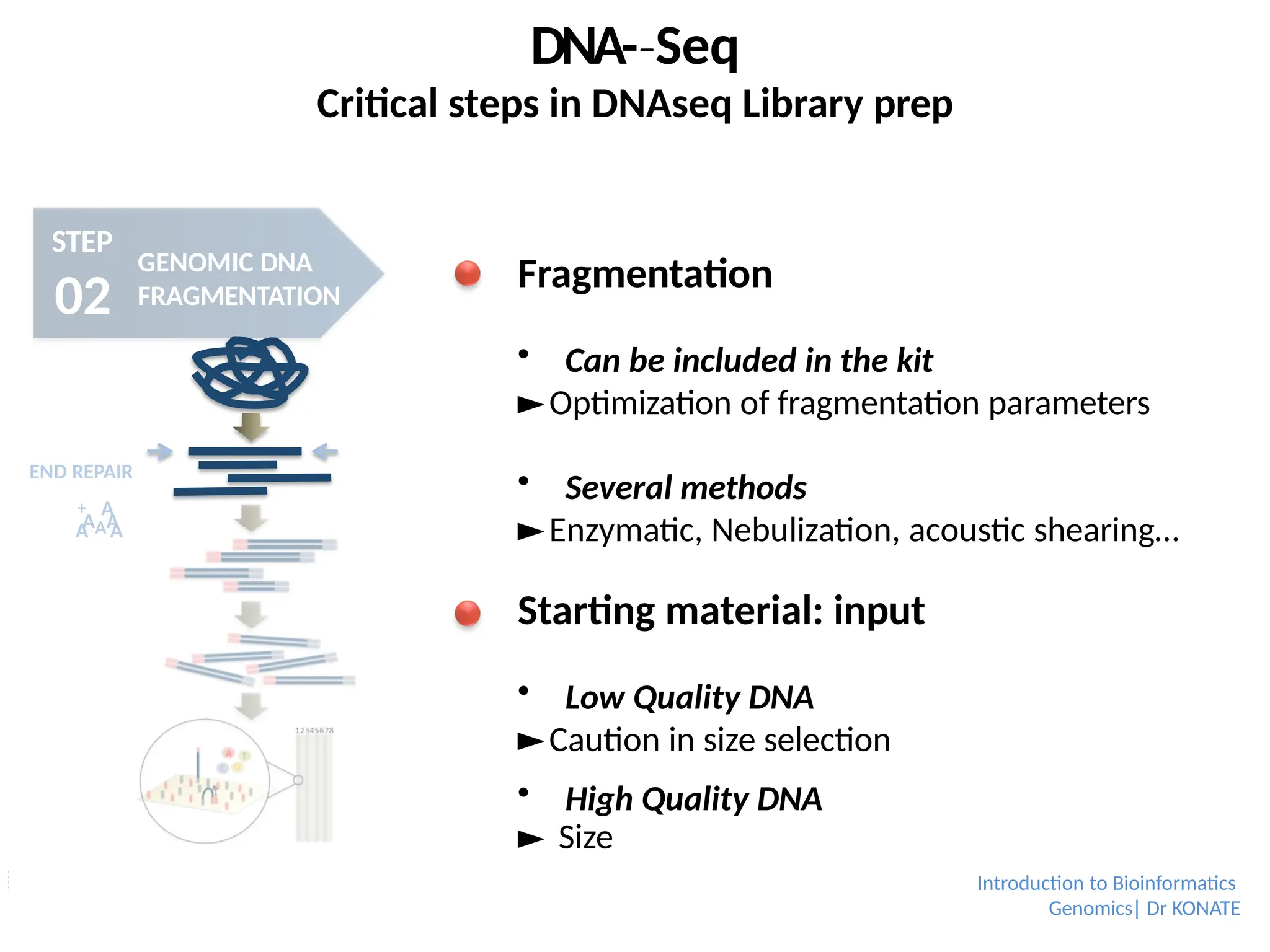
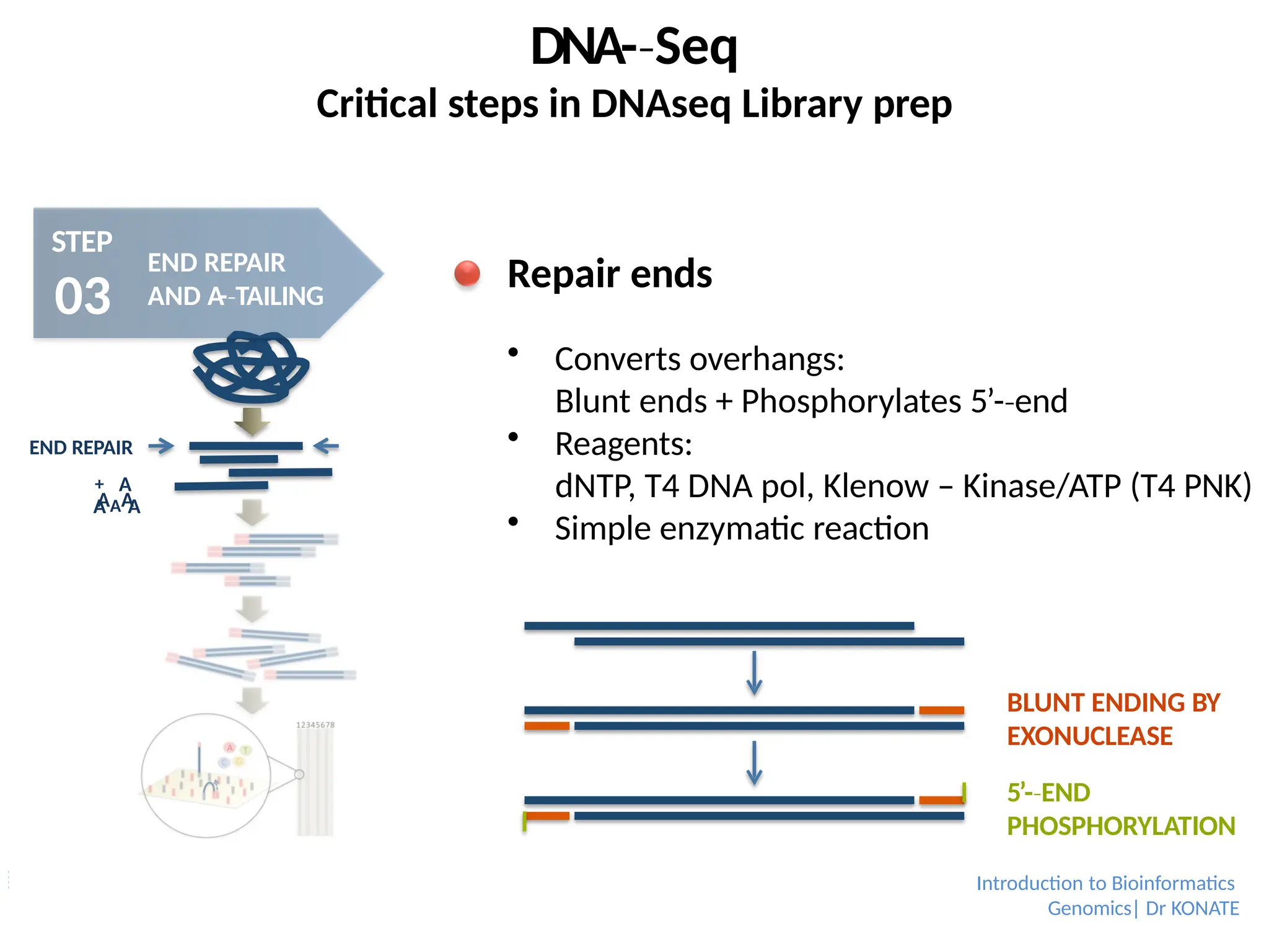
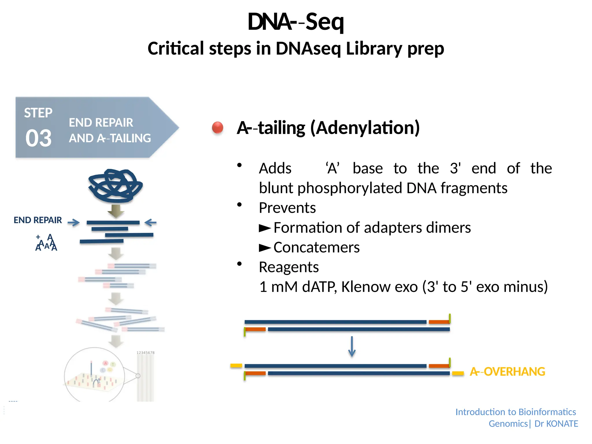
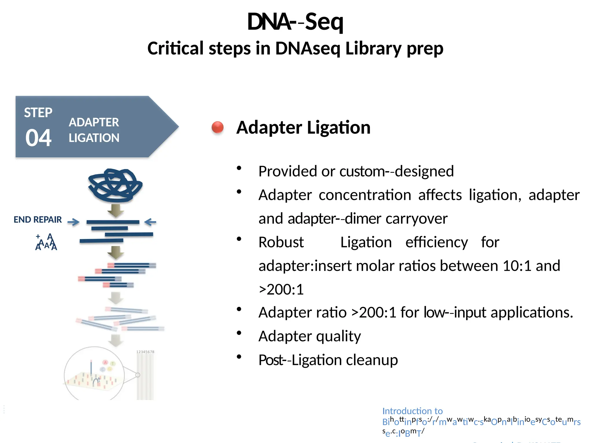
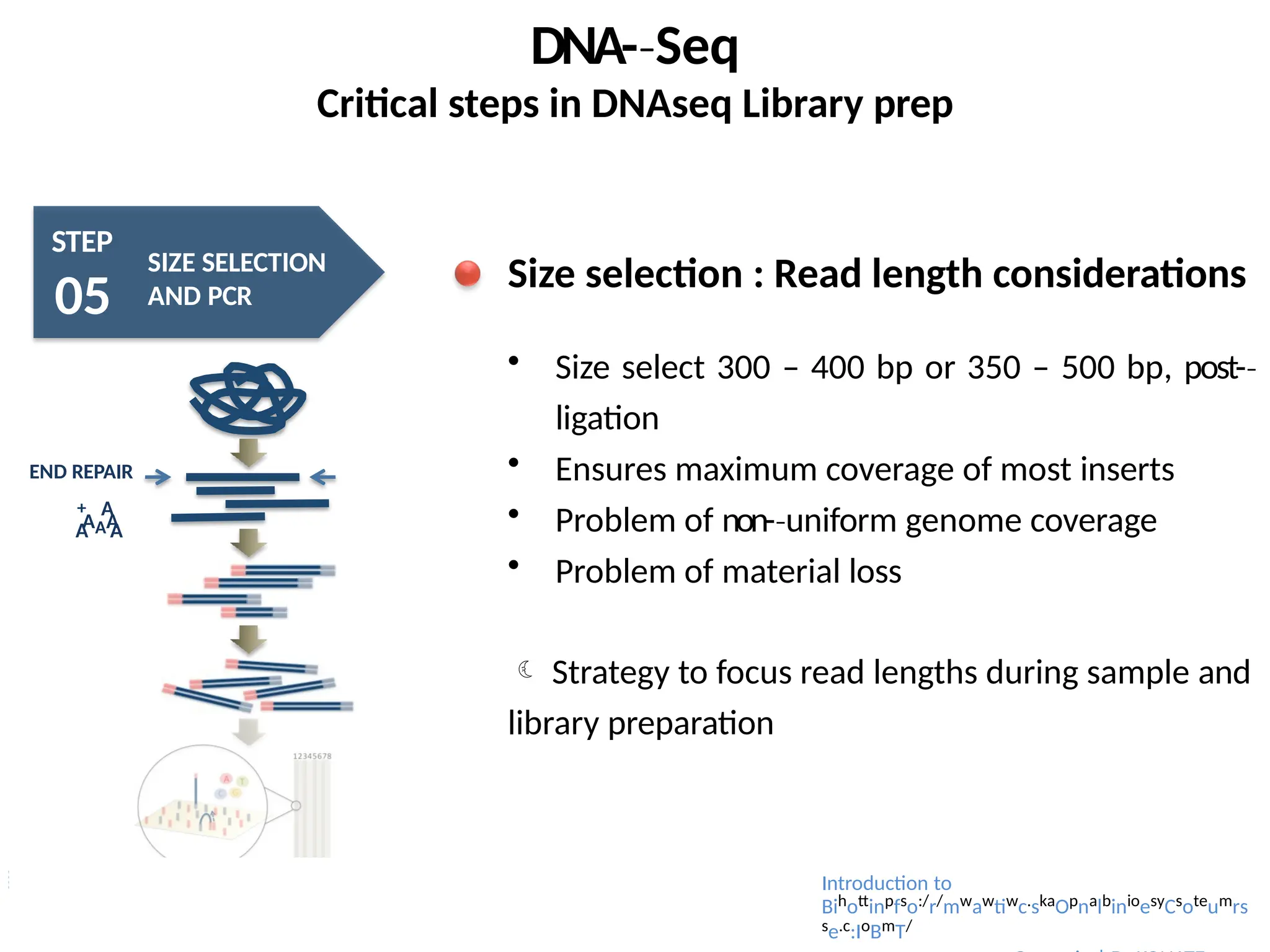
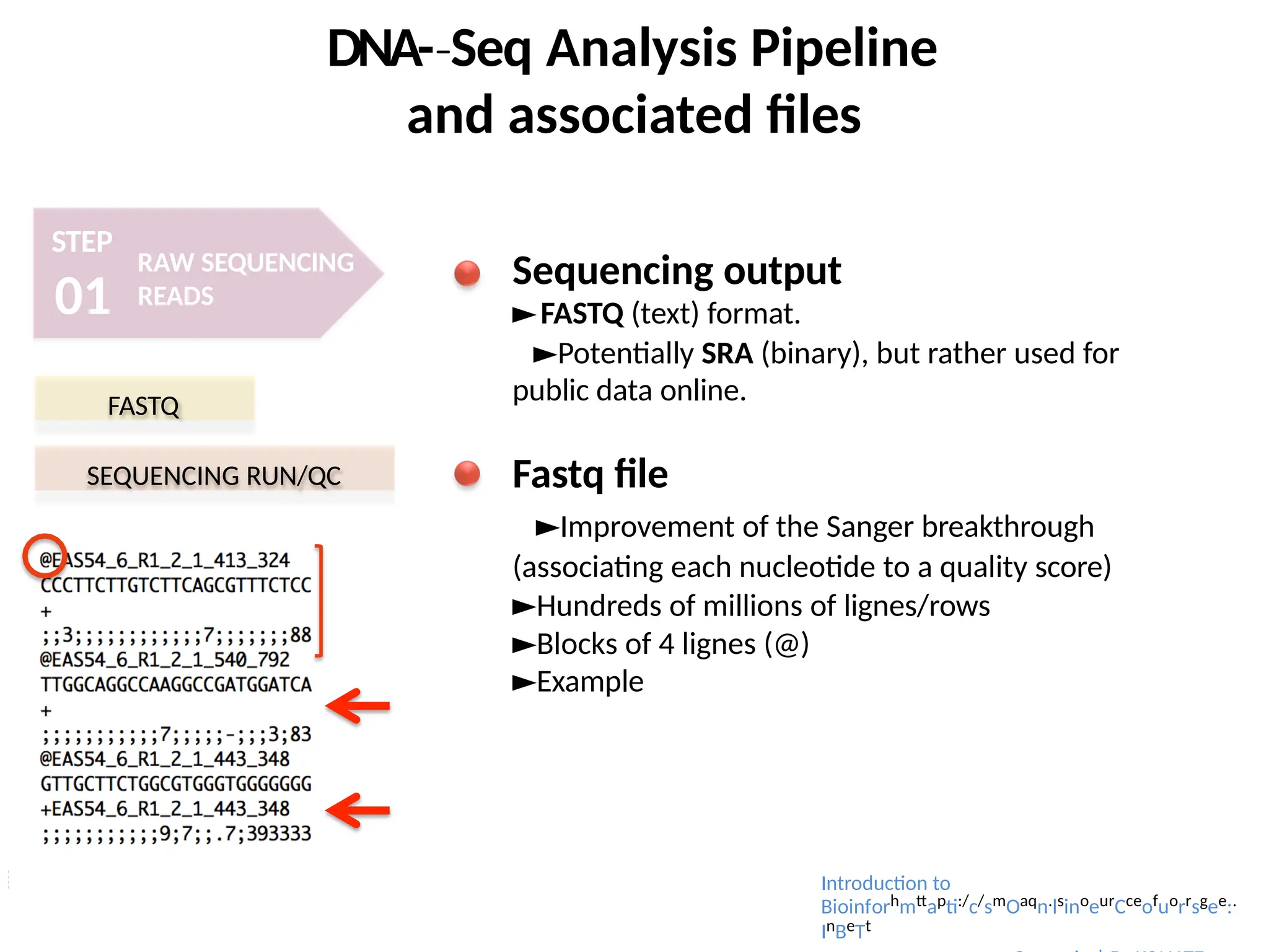
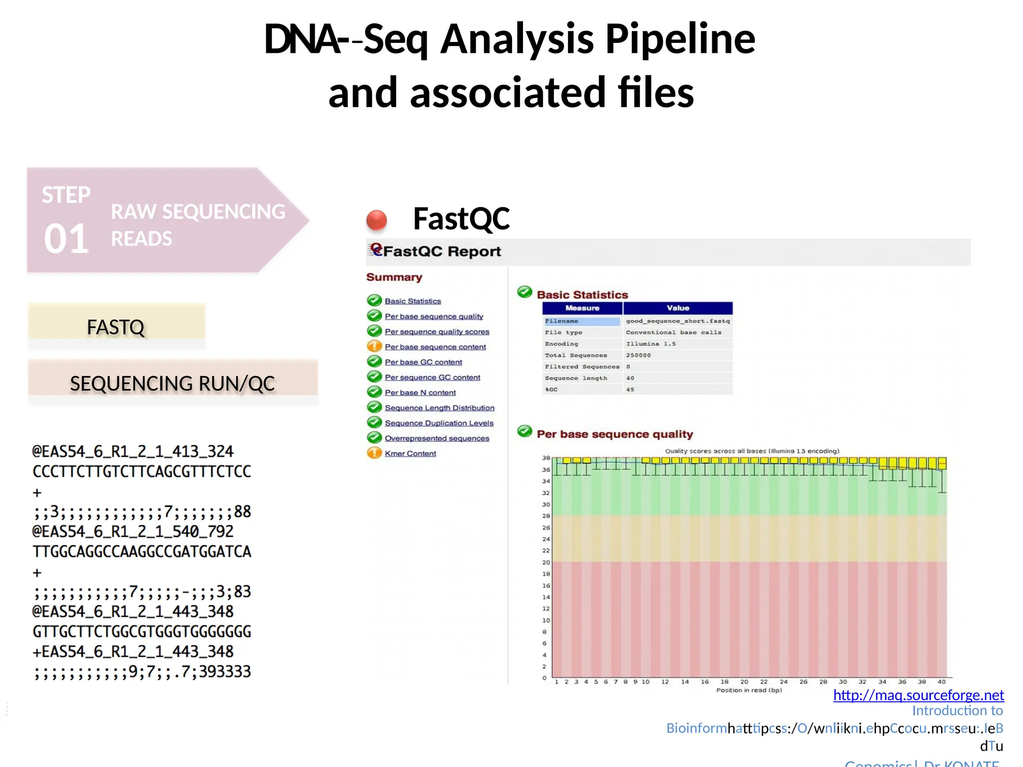
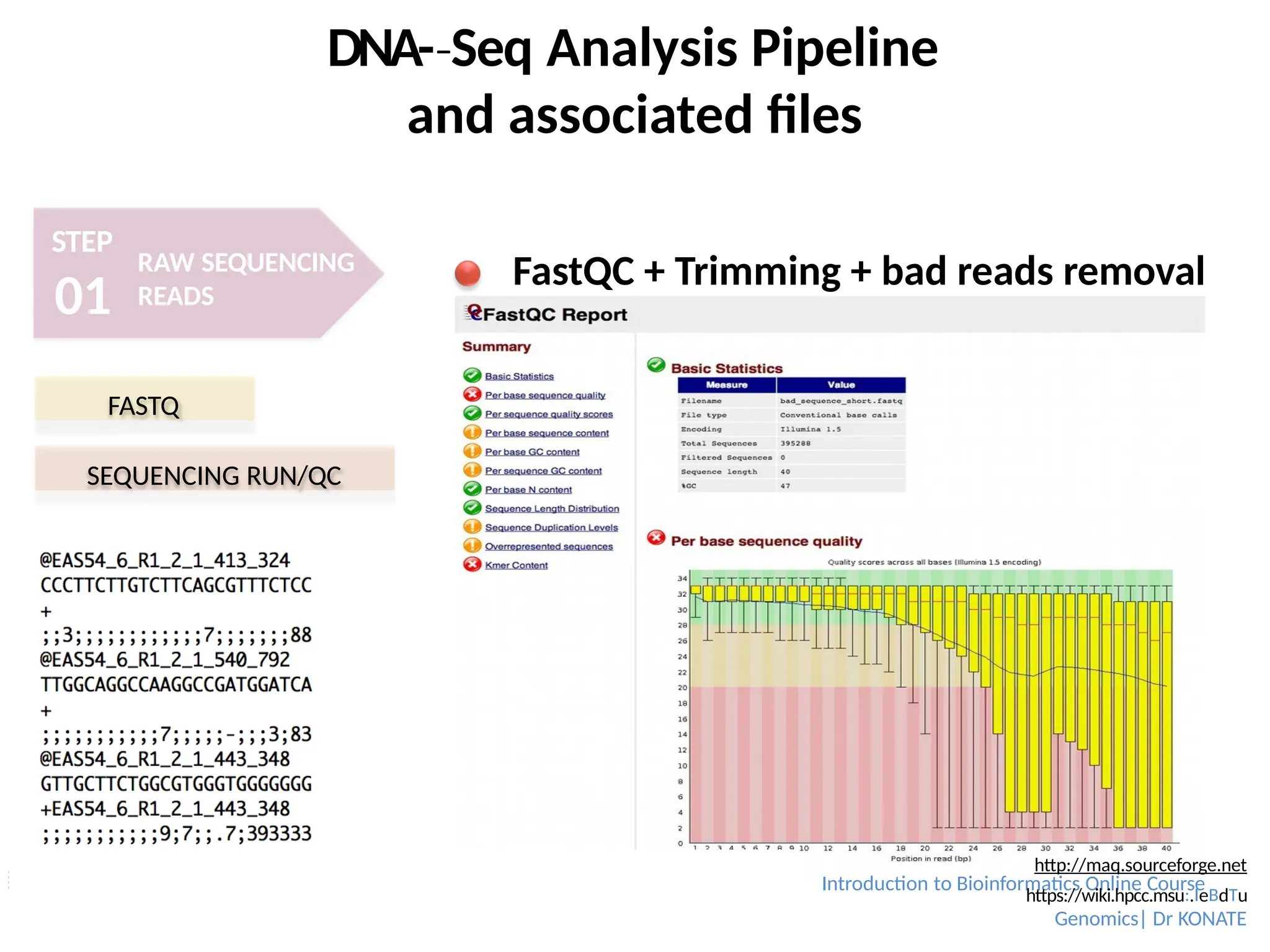
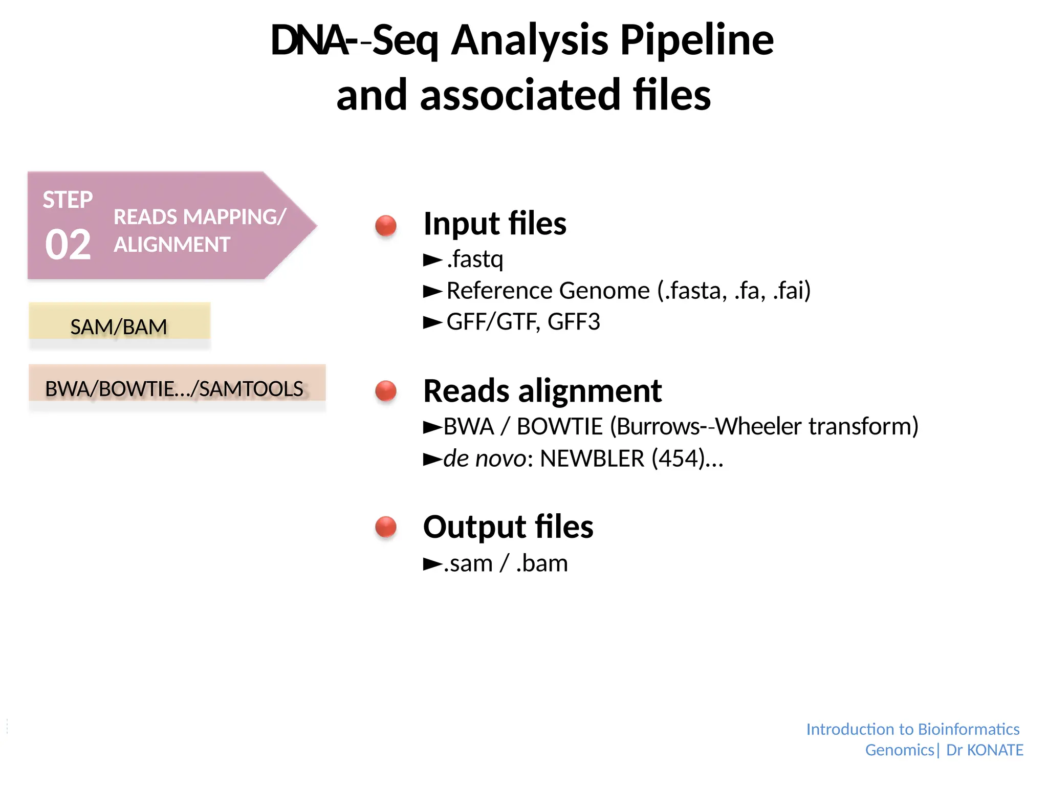
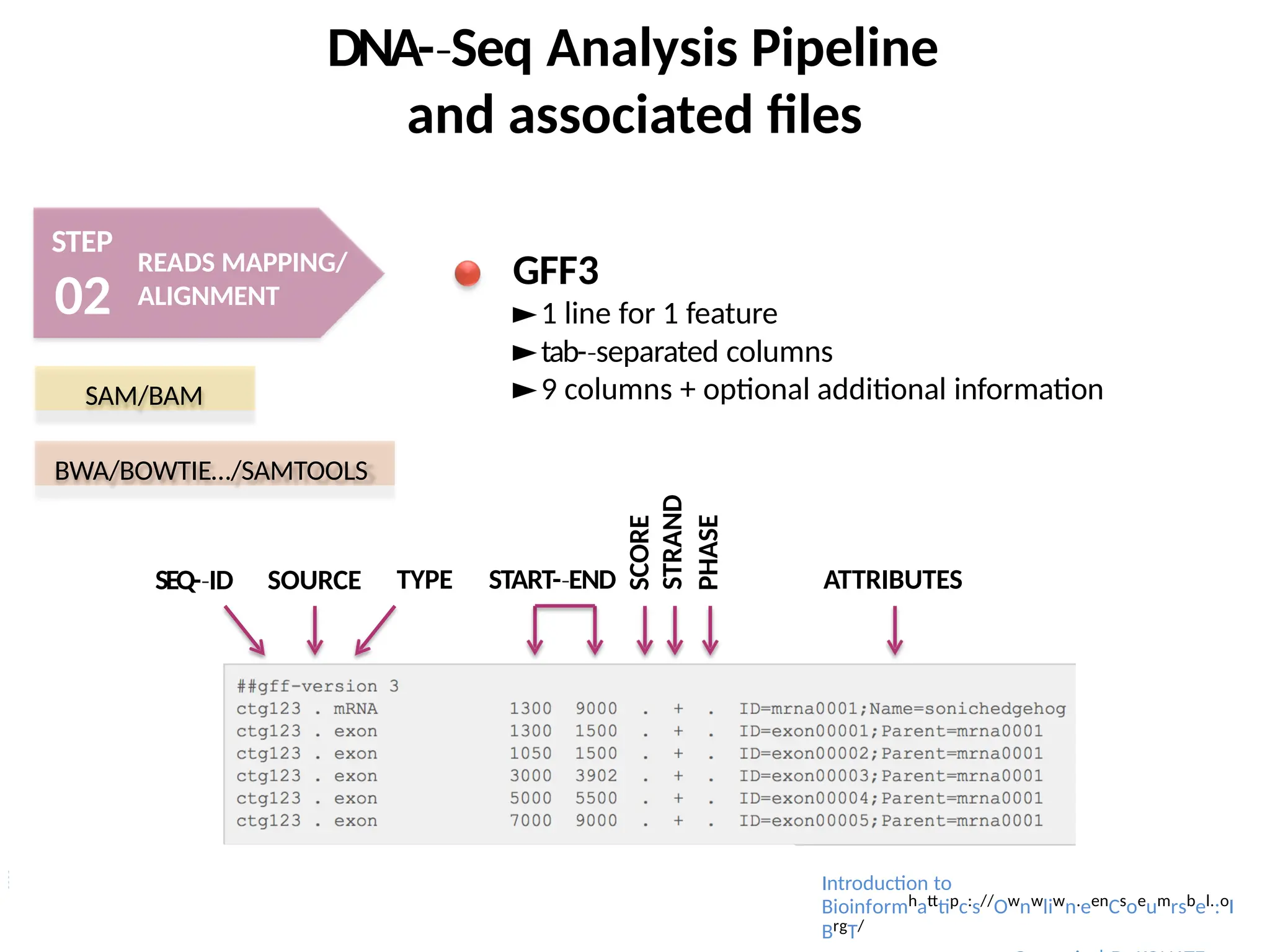
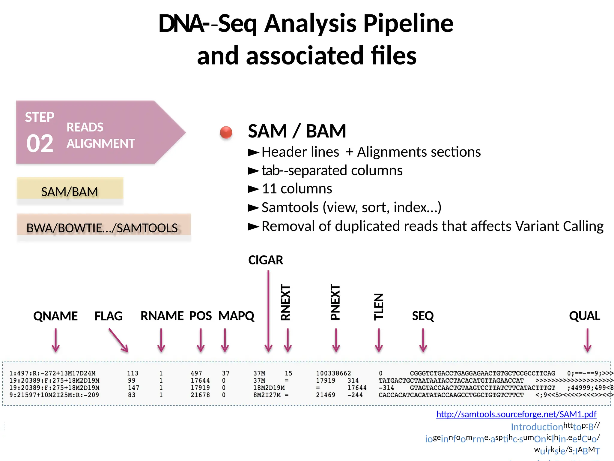
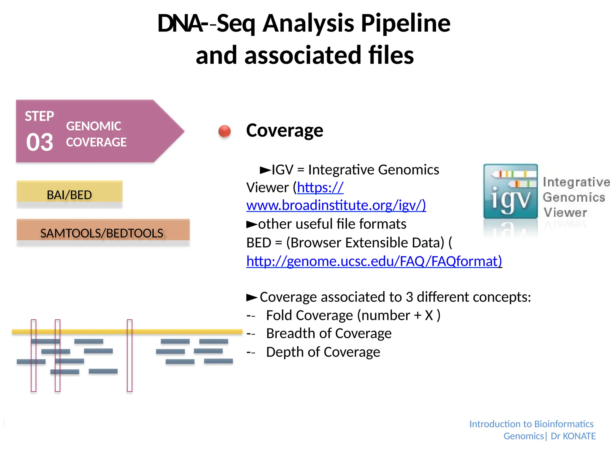
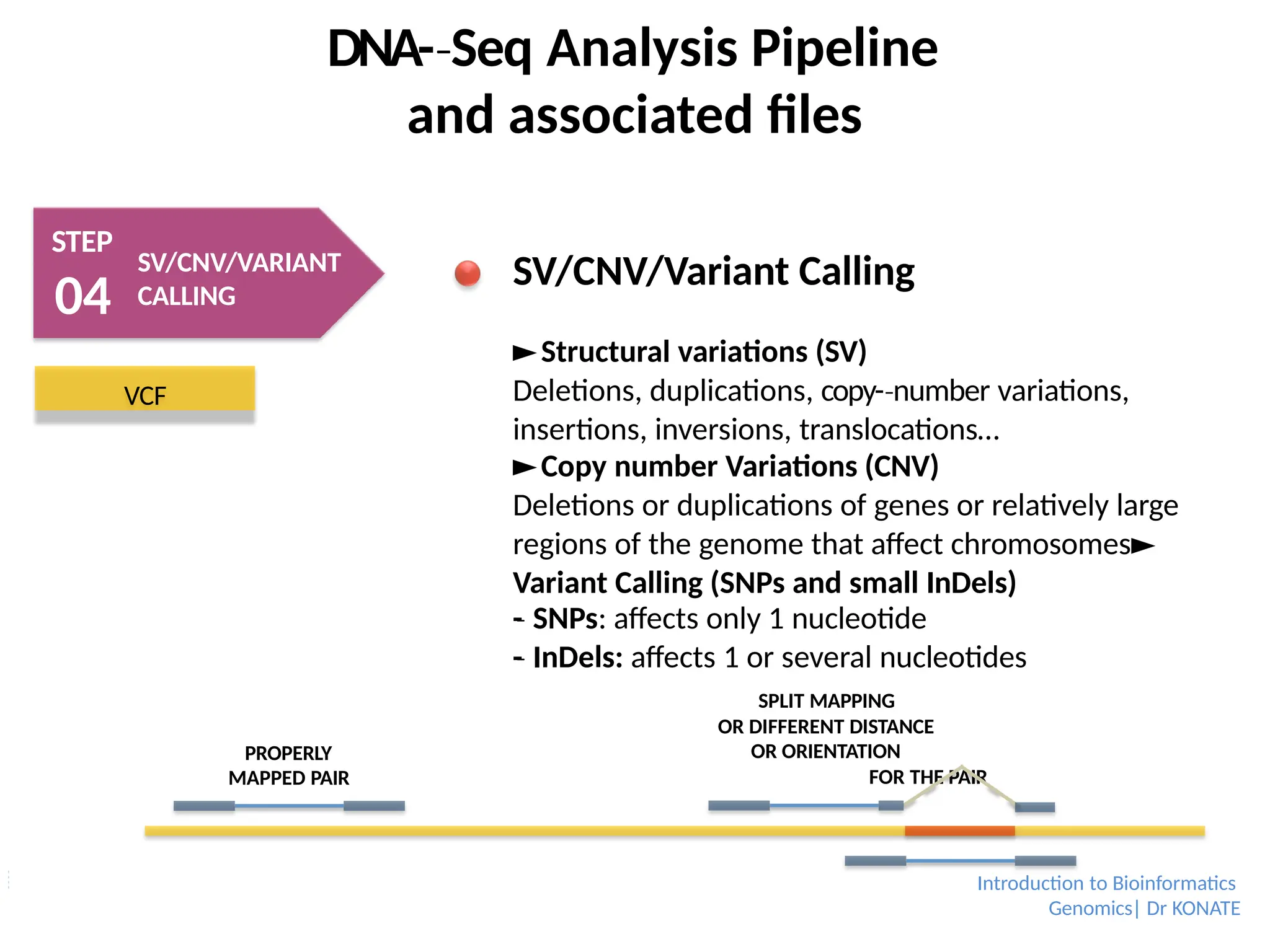
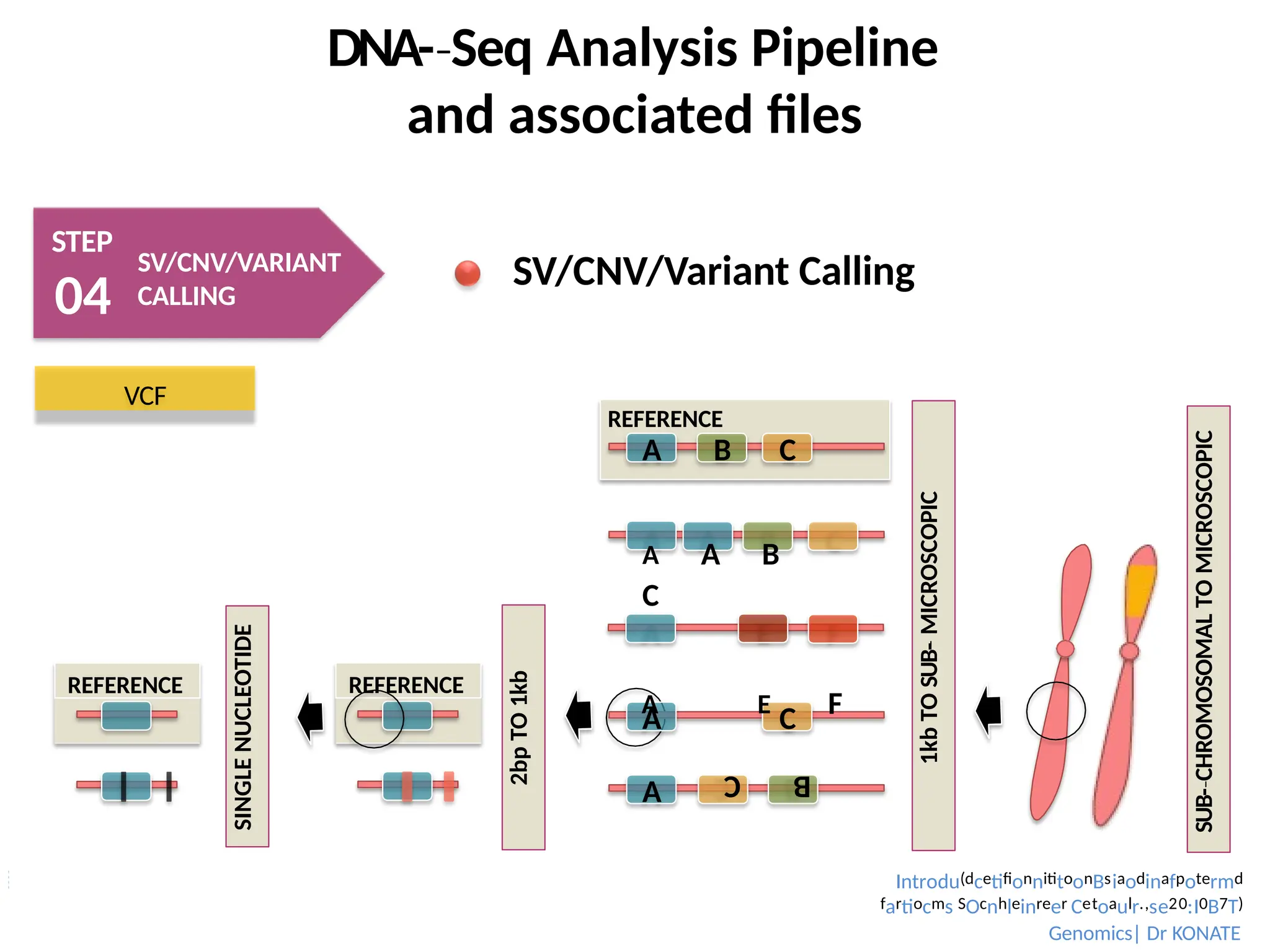
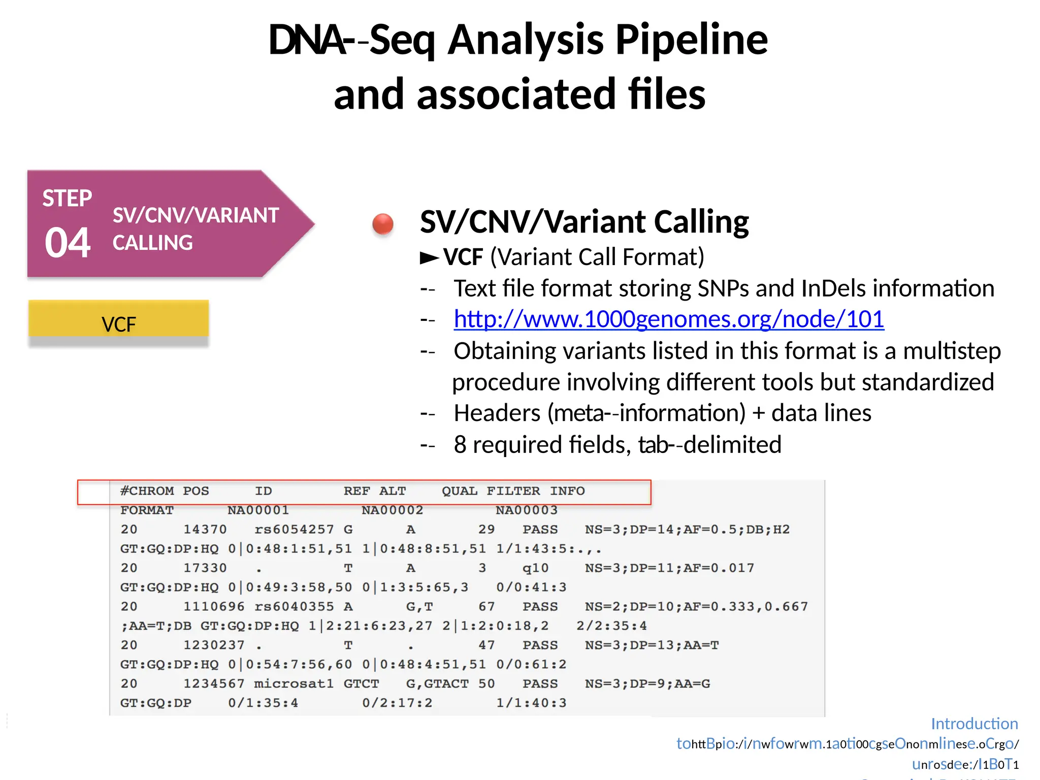
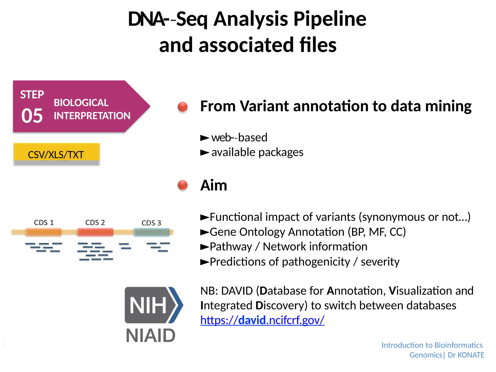
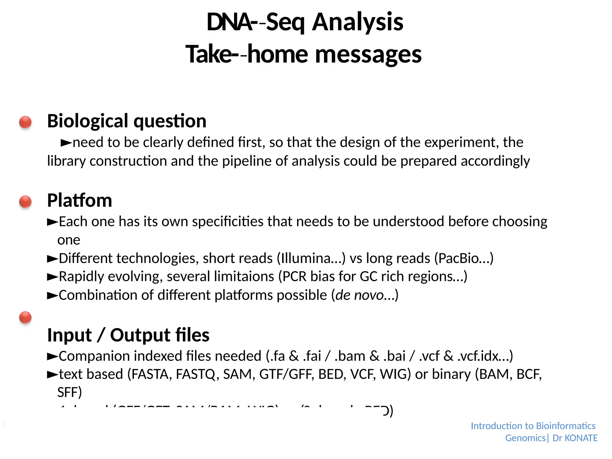
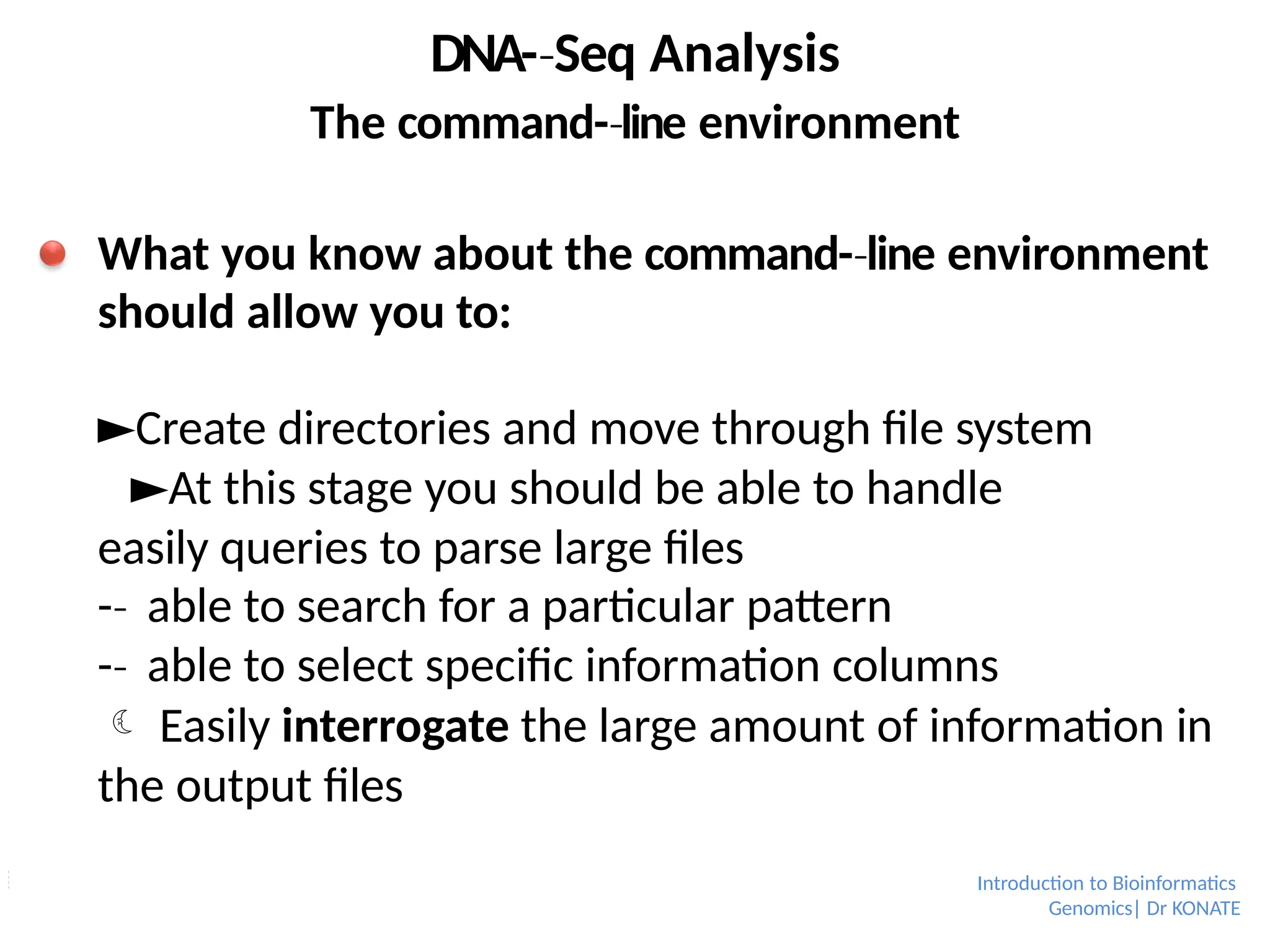
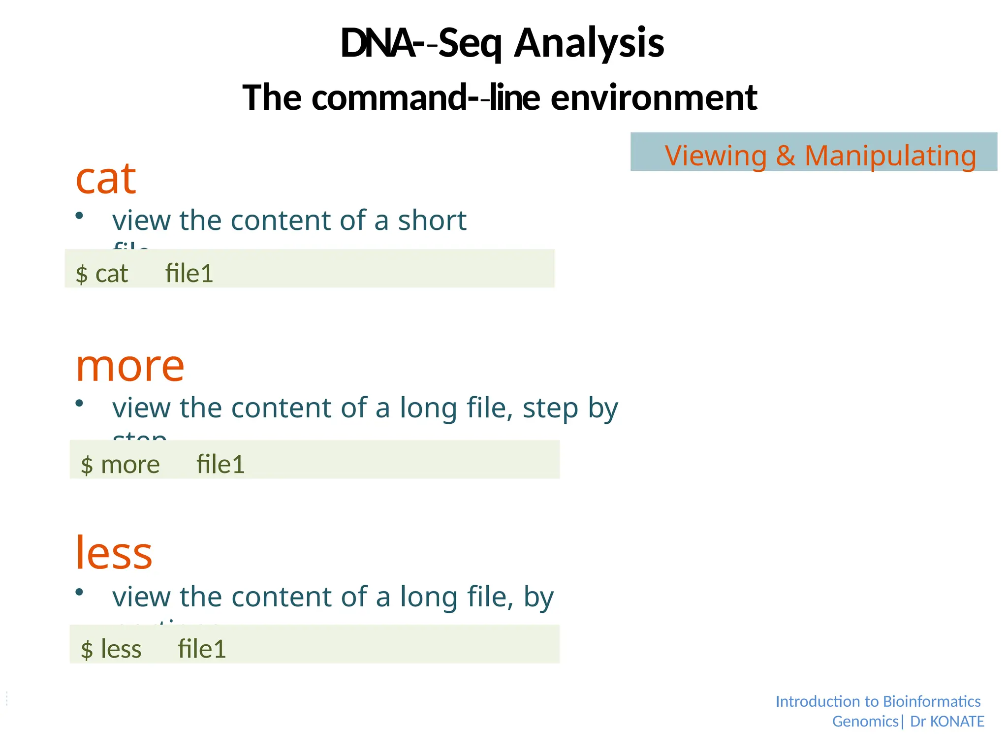
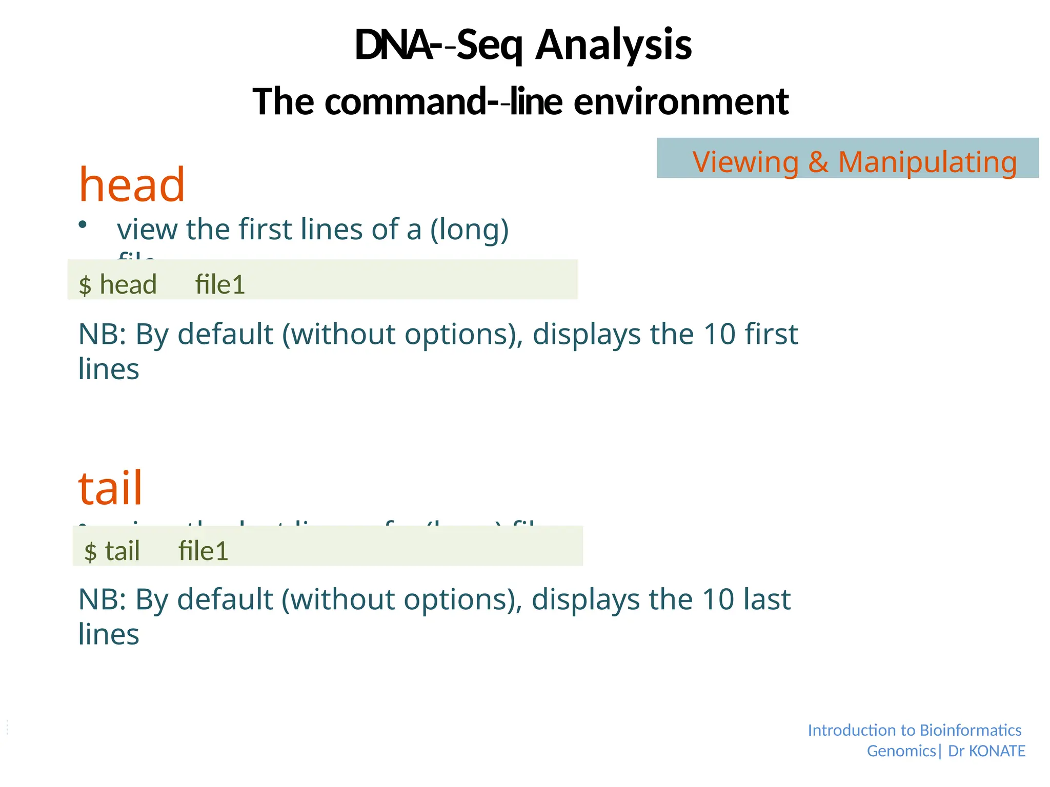
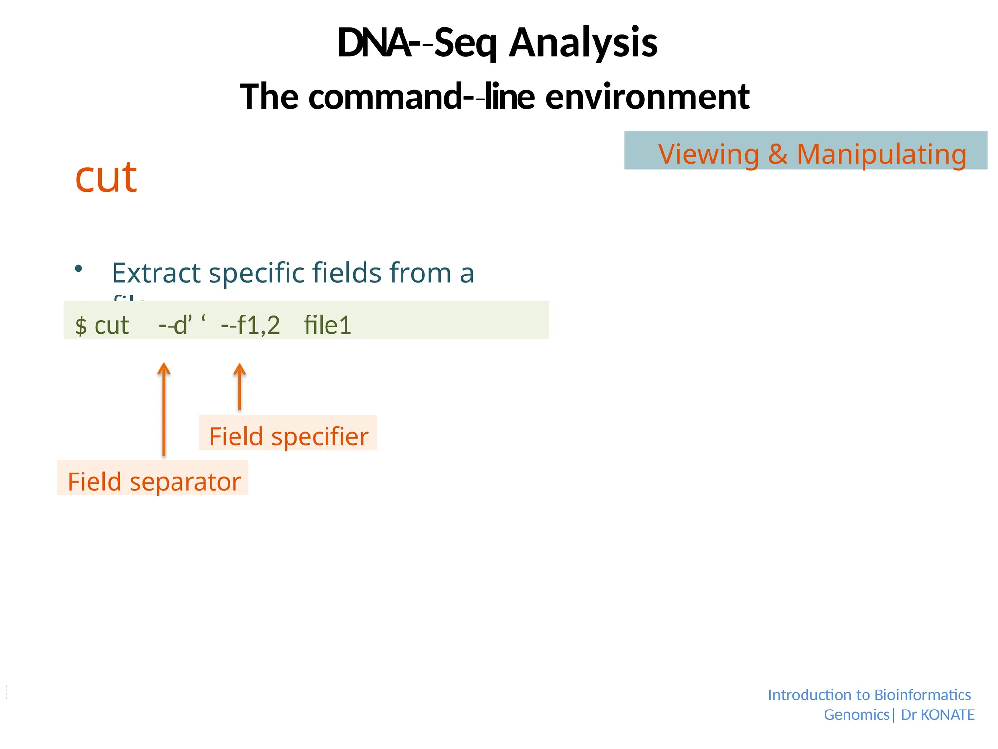
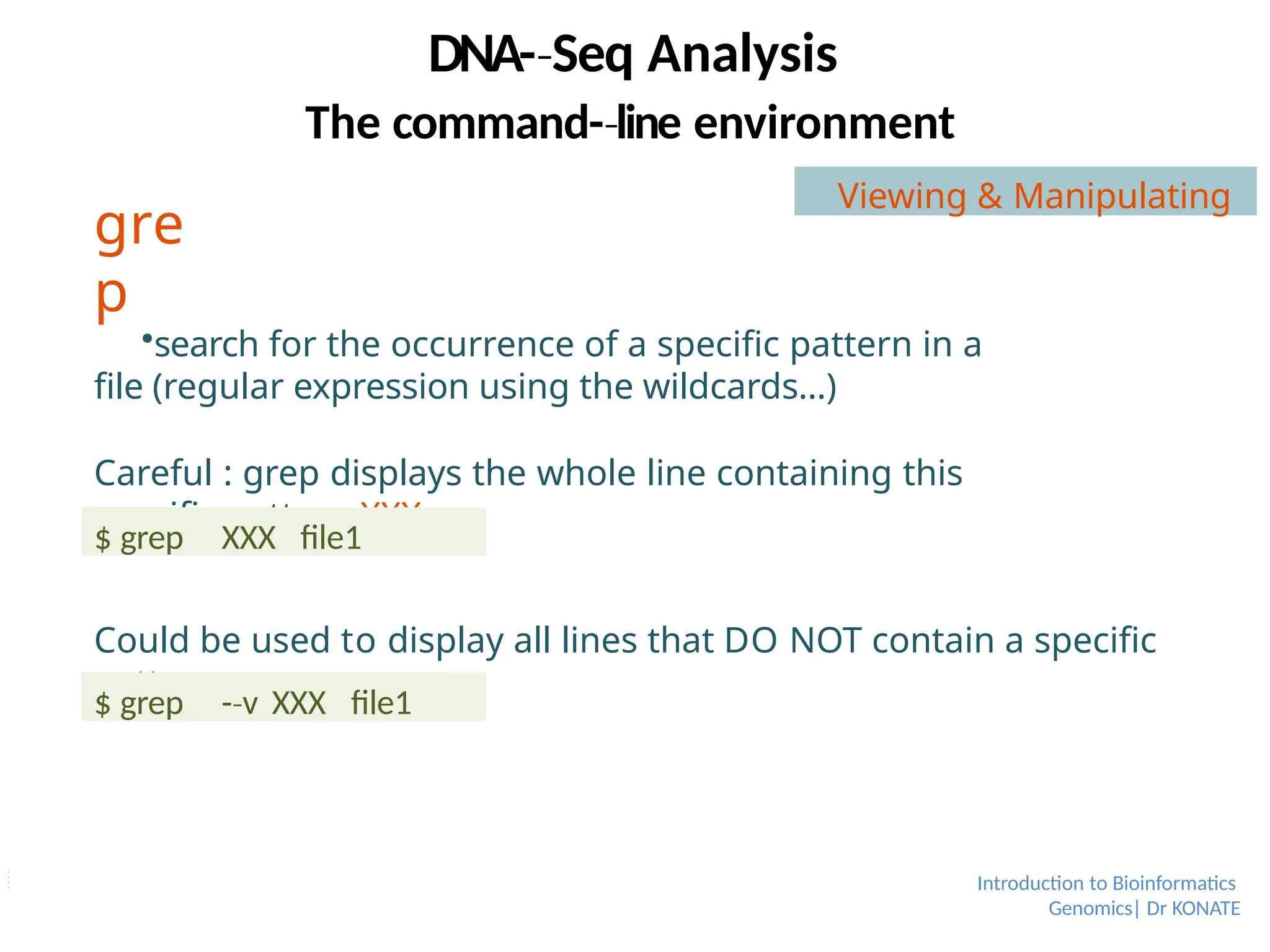
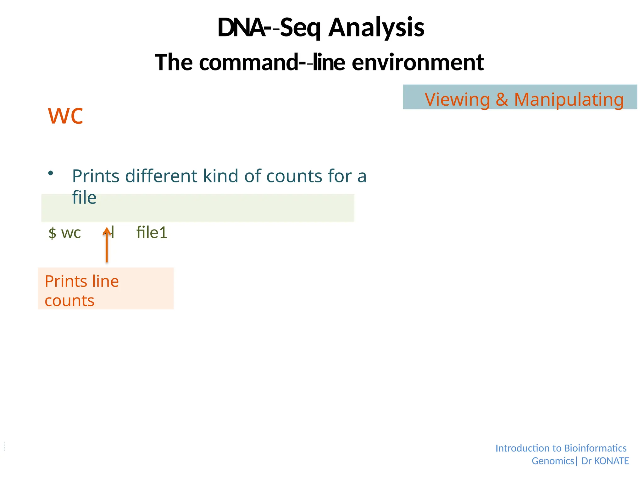
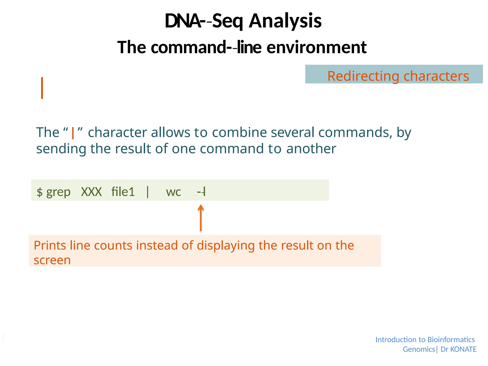
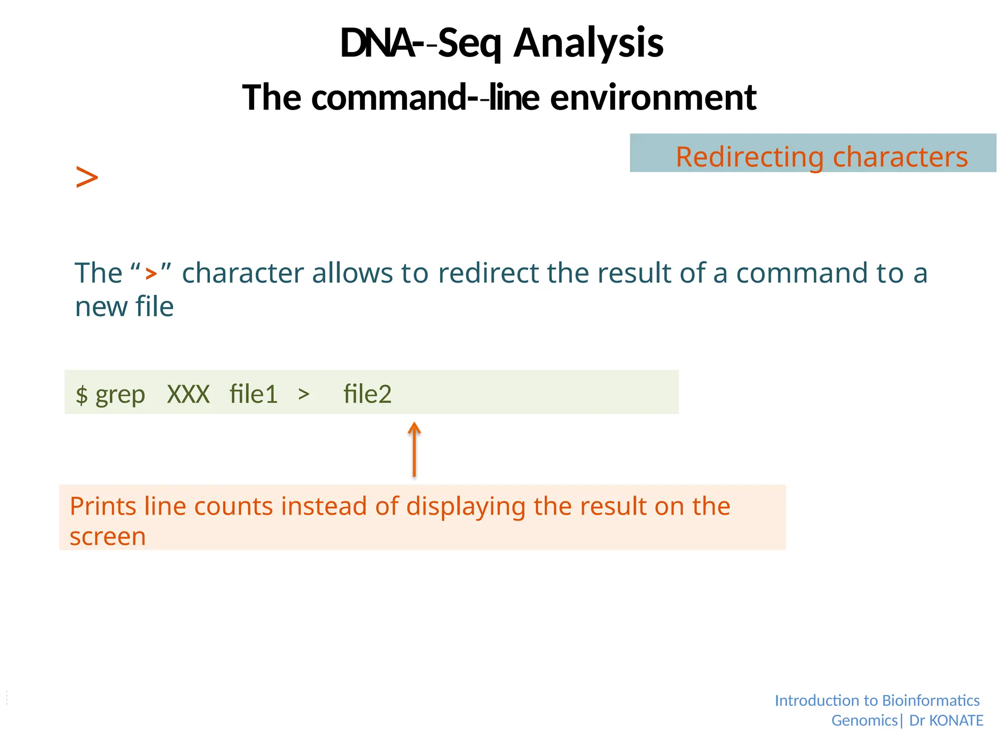
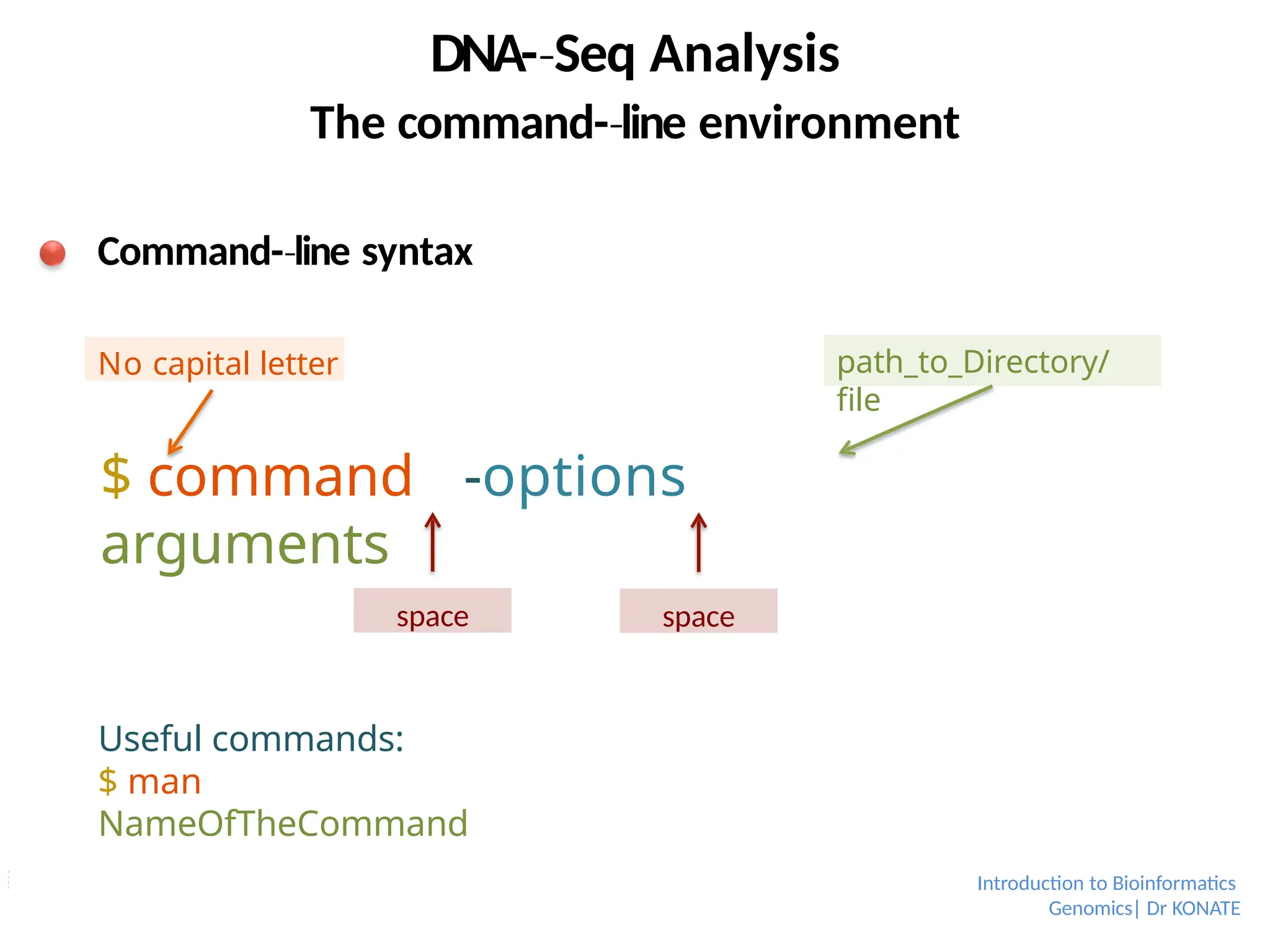
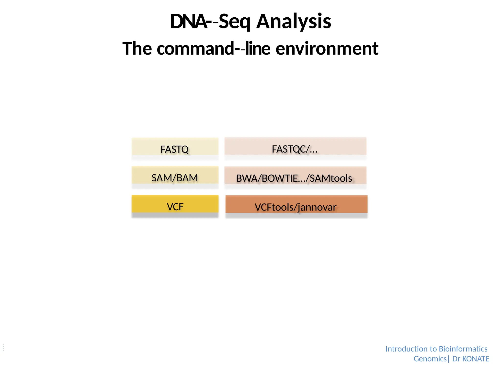
![To run FastQC (provided it is installed):
-
‐ specify the files you want to process on the command line
-
‐ FastQC will generate an HTML report for each file (embeded graphs)
FASTQ FASTQC/…
DNA-Seq
‐ Analysis
The command-line
‐ environment
fastqc seqfile1 seqfile2 .. seqfileN
fastqc [-o
‐ output dir] [--
‐(no)extract]
‐
fastqc --
‐ help
‐
-o
‐ –outdir
Create all output files in the specified
output directory (dir must already exist).
-
-
‐ extract
‐
Uncompress the zipped output
file in the same dir after being
created.
-
-
‐ noextract
‐
Do not uncompress the output file
after creating it.
Introduction to Bioinformatics
Genomics| Dr KONATE](https://image.slidesharecdn.com/module5session1-250516072911-3e48fda7/75/Module5-Genomics-sequencing-technologies-and-NGS-pptx-85-2048.jpg)