Download to read offline


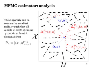


1) The document proposes a Model-Free Monte Carlo (MFMC) estimator to evaluate the performance of a policy in a discrete-time stochastic optimal control problem when the system model is unknown. 2) The MFMC estimator constructs simulated trajectories from a sample of one-step transitions to estimate the expected return, mimicking a standard Monte Carlo approach. 3) Analysis shows the bias and variance of the MFMC estimator converge to those of the Monte Carlo estimator as the number of transitions increases.