This document summarizes techniques for making deep learning models more efficient, including pruning, weight sharing, quantization, low-rank approximation, and Winograd transformations. It provides examples of applying these techniques to convolutional neural networks to reduce model size by up to 49x while maintaining accuracy. Specific techniques discussed include clustering weights to share values, quantizing weights to fewer bits, pruning low-impact connections, and iteratively retraining pruned models. Energy and computation reductions are achieved through smaller, lower-precision models with fewer operations.

2. 3
This image is licensed under CC-BY 2.0
This image is in the public domain
This image is in the public domain
This image is licensed under CC-BY 2.0

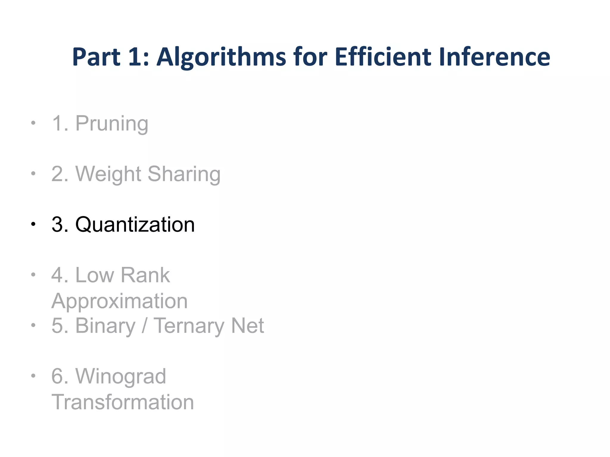
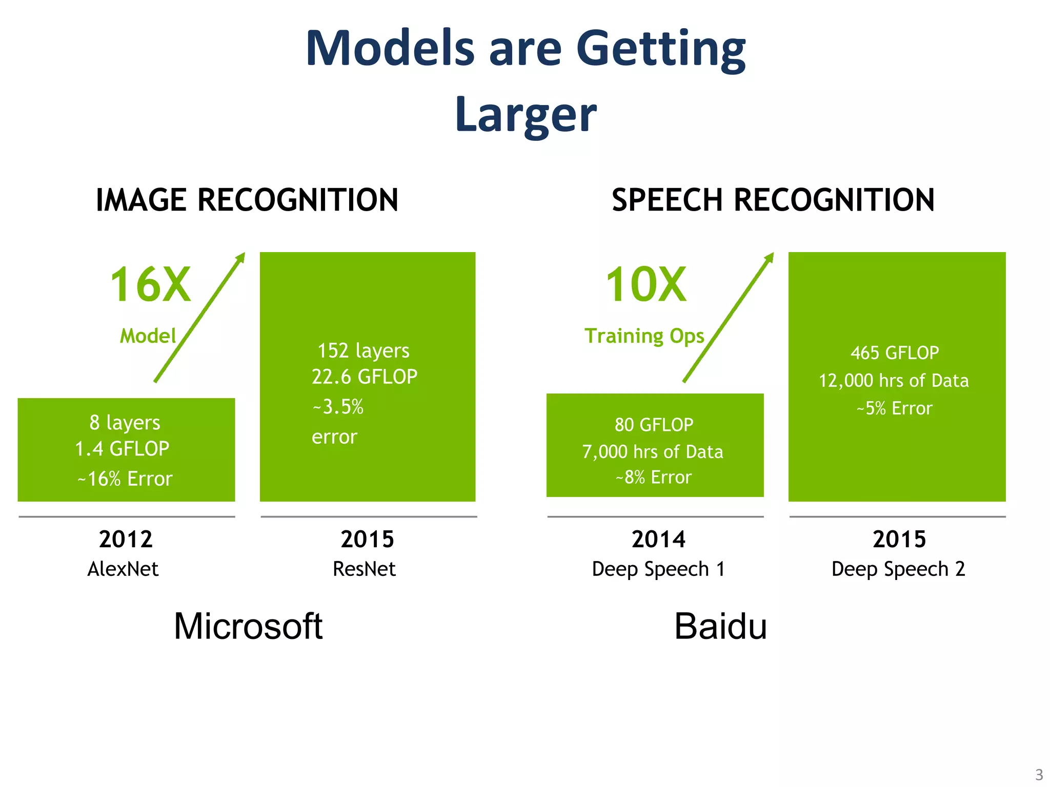
3. IMAGE RECOGNITION SPEECH RECOGNITION
2012
AlexNet
2015
ResNet
152 layers
22.6 GFLOP
~3.5%
error
8 layers
1.4 GFLOP
~16% Error
16X
Model
2014
Deep Speech 1
2015
Deep Speech 2
80 GFLOP
7,000 hrs of Data
~8% Error
10X
Training Ops
465 GFLOP
12,000 hrs of Data
~5% Error
Microsoft Baidu

4. Hard to distribute large models through over-the-air update
This image is licensed under CC-BY 2.0
App icon is in the public domain
Phone image is licensed under CC-BY 2.0

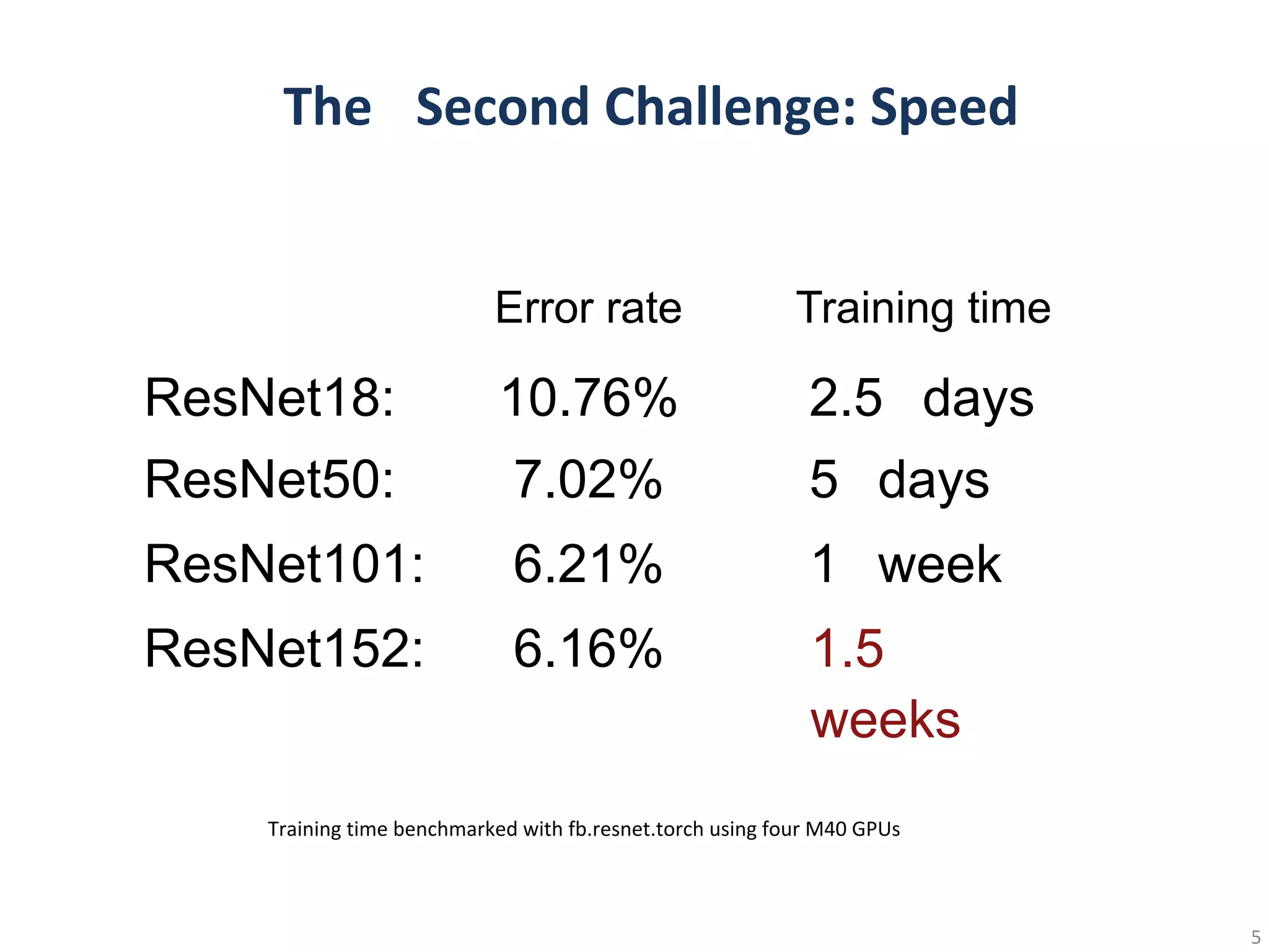
5. ResNet18: 10.76% 2.5 days
ResNet50: 7.02% 5 days
ResNet101: 6.21% 1 week
ResNet152: 6.16% 1.5
weeks
Error rate Training time

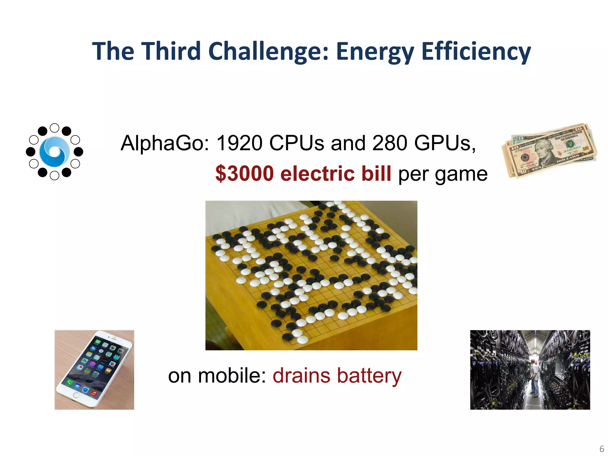
6. AlphaGo: 1920 CPUs and 280 GPUs,
$3000 electric bill per game
on mobile: drains battery

7. larger model => more memory reference => more energy

8. 1
Operatio
n
Energy [pJ]
32 bit int ADD 0.1
32 bit float ADD 0.9
32 bit Register File 1
32 bit int MULT 3.1
32 bit float MULT 3.7
32 bit SRAM Cache 5
32 bit DRAM Memory 640
Relative Energy Cost
1 10
=1000
100 1000
10000
larger model => more memory reference => more energy

9. Operation Energy[pJ
]
Relative Energy Cost
32 bit int AD 0.1
32 bit float ADD 0.9
32 bit Register File 1
32 bit int MULT 3.1
32 bit float MULT 3.7
32 bit SRAM Cache 5
32 bit DRAM Memory 640
1 10 100 1000 10000
how to make deep learning more efficient?
larger model => more memory reference => more energy

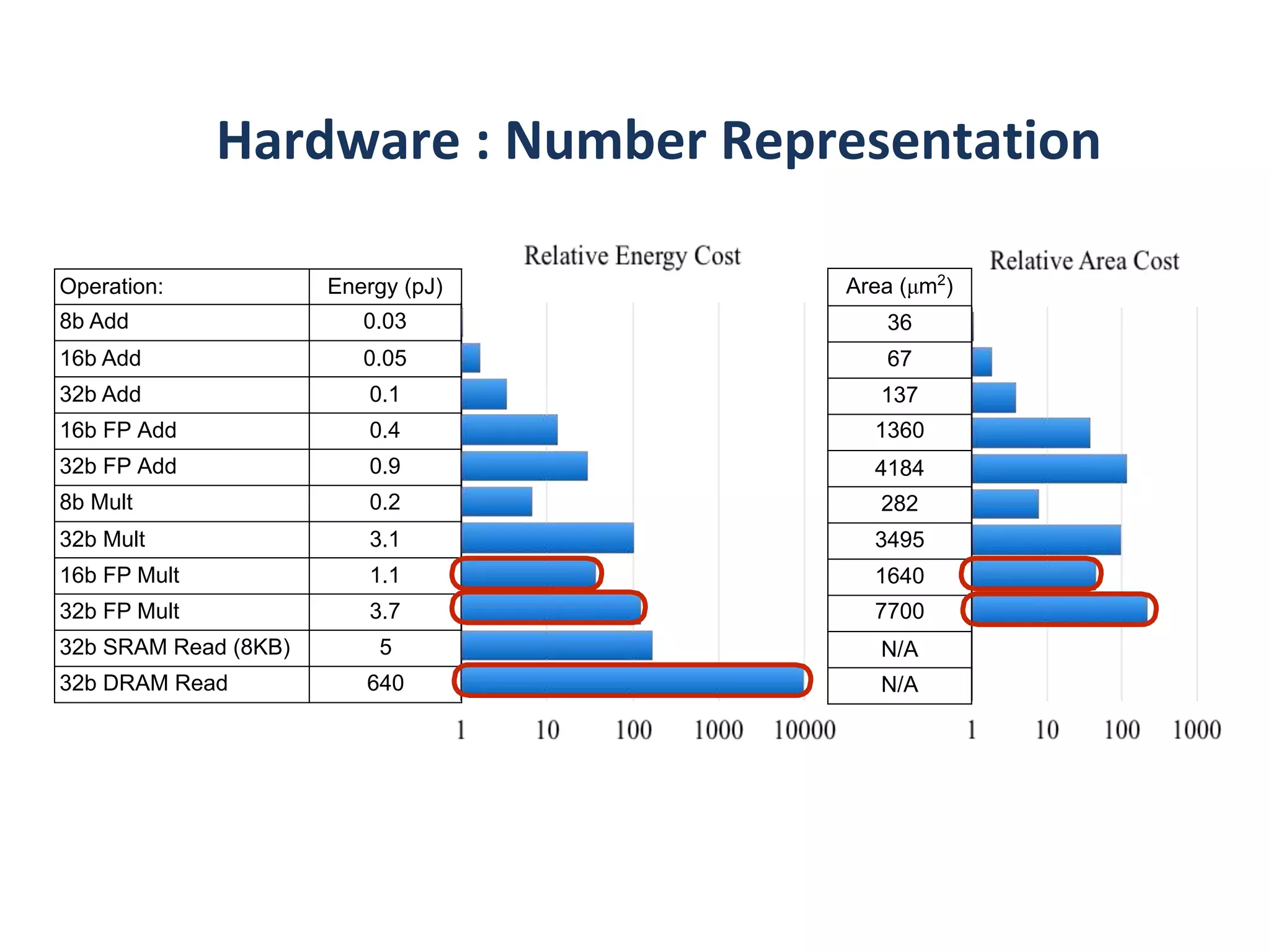
10. Operation: Energy (pJ)
8b Add 0.03
16b Add 0.05
32b Add 0.1
16b FP Add 0.4
32b FP Add 0.9
8b Mult 0.2
32b Mult 3.1
16b FP Mult 1.1
32b FP Mult 3.7
32b SRAM Read (8KB) 5
32b DRAM Read 640
Area (μm2
)
36
67
137
1360
4184
282
3495
1640
7700
N/A
N/A

11. •
6. Winograd
Transformation
•
1. Pruning
• 2. Weight Sharing
• 3. Quantization
• 4. Low Rank
Approximation
• 5. Binary / Ternary Net

12. 6. Winograd
Transformation
•
• 1. Pruning
• 2. Weight Sharing
• 3. Quantization
• 4. Low Rank
Approximation
• 5. Binary / Ternary Net

13. 13

14. 60 Million
6M
-0.01x2
+x+1
14

15. 15
AccuracyLoss
0.5%
0.0%
-0.5%
-1.0%
-1.5%
-2.0%
-2.5%
-3.0%
-3.5%
-4.0%
-4.5%
40% 50% 60% 70% 80%
Parameters Pruned Away
90% 100%

16. AccuracyLoss -0.5%
-1.0%
-1.5%
-2.0%
-2.5%
-3.0%
-3.5%
-4.0%
-4.5%
0.5%
0.0%
40% 50% 60% 70% 80%
Parameters Pruned Away
90% 100%
Pruning
16

17. AccuracyLoss
0.5%
0.0%
-0.5%
-1.0%
-1.5%
-2.0%
-2.5%
-3.0%
-3.5%
-4.0%
-4.5%
Parameters Pruned
Away
40% 50% 60% 70% 80% 90% 100%
Pruning Pruning+Retraining
17

18. AccuracyLoss
0.5%
0.0%
-0.5%
-1.0%
-1.5%
-2.0%
-2.5%
-3.0%
-3.5%
-4.0%
-4.5%
40% 50% 60% 70% 80%
Parameters Pruned Away
100%
Pruning Pruning+Retraining Iterative Pruning and Retraining
90%
18

19. Pruning RNNand LSTM
19

20. • Original:a basketball playerin a white uniform
is playing with a ball
• Pruned 90%: a basketball player in a white uniform
is playing with a basketball
• Original : a brown dog is running through a grassy
field
• Pruned 90%: a brown dog is running through a
grassy area
•
•
Original : a soccer player in red is running in the field
Pruned 95%: a man in a red shirt and black and
white black shirt is running through a field
•
•
Original : a man is riding a surfboard on a wave
Pruned 90%: a man in a wetsuit is riding a wave on a
beach
95%
20
90%
90%
90%

21. 50 Trillion
Synapses
500
Trillion
Synapses
1000
Trillion
Synapses
Newborn 1 year old Adolescent
This image is in the public domain This image is in the public domain This image is in the public domain
21

22. Before Pruning After Pruning After Retraining
22

23. • 1. Pruning
• 2. Weight Sharing
• 3. Quantization
• 4. Low Rank
Approximation
• 5. Binary / Ternary Net
• 6. Winograd
Transformation

24. ,
2.09, 2.12, 1.92,
1.87
2.0

25. Cluster the Weights
Generate Code Book
Quantize the Weights
with Code Book
Retrain Code Book
,
32 bit
4bit
2.09, 2.12, 1.92, 1.87
2.0

26. ,
2.09 -0.98 1.48 0.09
0.05 -0.14 -1.08 2.12
-0.91 1.92 0 -1.03
1.87 0 1.53 1.49
weights
(32 bit float)
gradient
-0.03 -0.01 0.03 0.02 -0.03 0.12 0.02 -0.07 0.04
-0.01 0.01 -0.02 0.12
group by
0.03 0.01
-0.02 reduce
0.02
-0.01 0.02 0.04 0.01 0.02 -0.01 0.01 0.04 -0.02 0.04
-0.07 -0.02 0.01 -0.02 -0.01 -0.02 -0.01 0.01 -0.03
lr
cluster index
(2 bit uint)
centroids
3 0 2 1
3:
2.00
cluster
1 1 0 3 2: 1.50
0 3 1 0
1:
0.00
3 1 2 2
0:
-1.00

27. 2.09 -0.98 1.48 0.09
0.05 -0.14 -1.08 2.12
-0.91 1.92 0 -1.03
1.87 0 1.53 1.49
cluster
cluster index
(2 bit uint)
3 0 2 1
1 1 0 3
0 3 1 0
3 1 2 2
gradient
-0.03 -0.01 0.03 0.02 -0.03 0.12 0.02 -0.07 0.04
-0.01 0.01 -0.02 0.12
group by
0.03 0.01
-0.02 reduce
0.02
-0.01 0.02 0.04 0.01 0.02 -0.01 0.01 0.04 -0.02 0.04
-0.07 -0.02 0.01 -0.02 -0.01 -0.02 -0.01 0.01 -0.03
1:
0:
2:
weights
(32 bit float)centroids
3: 2.00
1.50
0.00
-1.00
,

28. 2.09 -0.98 1.48 0.09
0.05 -0.14 -1.08 2.12
-0.91 1.92 0 -1.03
1.87 0 1.53 1.49
cluster
weights
(32 bit float) centroids
3 0 2 1
1 1 0 3
0 3 1 0
3 1 2 2
cluster index
(2 bit uint)
gradient
-0.03 -0.01 0.03 0.02 -0.03 0.12 0.02 -0.07 0.04
-0.01 0.01 -0.02 0.12
group by
0.03 0.01
-0.02 reduce
0.02
-0.01 0.02 0.04 0.01 0.02 -0.01 0.01 0.04 -0.02 0.04
-0.07 -0.02 0.01 -0.02 -0.01 -0.02 -0.01 0.01 -0.03
1:
0:
2:
3: 2.00
1.50
0.00
-1.00
,

29. 2.09 -0.98 1.48 0.09
0.05 -0.14 -1.08 2.12
-0.91 1.92 0 -1.03
1.87 0 1.53 1.49
-0.03 -0.01 0.03 0.02
-0.01 0.01 -0.02 0.12
-0.01 0.02 0.04 0.01
-0.07 -0.02 0.01 -0.02
cluster
weights
(32 bit float) centroids
gradient
3 0 2 1
1 1 0 3
0 3 1 0
3 1 2 2
cluster index
(2 bit uint)
-0.03 0.12 0.02 -0.07 0.04
group by
0.03 0.01
-0.02 reduce
0.02
0.02 -0.01 0.01 0.04 -0.02 0.04
-0.01 -0.02 -0.01 0.01 -0.03
1:
0:
2:
3: 2.00
1.50
0.00
-1.00
,

30. 2.09 -0.98 1.48 0.09
0.05 -0.14 -1.08 2.12
-0.91 1.92 0 -1.03
1.87 0 1.53 1.49
-0.03 -0.01 0.03 0.02
-0.01 0.01 -0.02 0.12
-0.01 0.02 0.04 0.01
-0.07 -0.02 0.01 -0.02
cluster
weights
(32 bit float) centroids
gradient
3 0 2 1
1 1 0 3
0 3 1 0
3 1 2 2
cluster index
(2 bit uint)
2.00
1.50
0.00
-1.00
group by
-0.03 0.12 0.02 -0.07
0.03 0.01 -0.02 r
0.02 -0.01 0.01 0.04 -0.02
-0.01 -0.02 -0.01 0.01
0.04
educe
0.02
0.04
-0.03
1:
0:
2:
3:
,

31. 2.09 -0.98 1.48 0.09
0.05 -0.14 -1.08 2.12
-0.91 1.92 0 -1.03
1.87 0 1.53 1.49
-0.03 -0.01 0.03 0.02
-0.01 0.01 -0.02 0.12
-0.01 0.02 0.04 0.01
-0.07 -0.02 0.01 -0.02
cluster
weights
(32 bit float) centroids
gradient
3 0 2 1
1 1 0 3
0 3 1 0
3 1 2 2
cluster index
(2 bit uint)
2.00
1.50
0.00
-1.00
group by
-0.03 0.12 0.02 -0.07
0.03 0.01 -0.02 r
0.02 -0.01 0.01 0.04 -0.02
-0.01 -0.02 -0.01 0.01
0.04
0.02
0.04
-0.03
educe
1:
lr0:
2:
3:

32. 2.09 -0.98 1.48 0.09
0.05 -0.14 -1.08 2.12
-0.91 1.92 0 -1.03
1.87 0 1.53 1.49
-0.03 -0.01 0.03 0.02
-0.01 0.01 -0.02 0.12
-0.01 0.02 0.04 0.01
-0.07 -0.02 0.01 -0.02
cluster
weights
(32 bit float) centroids
gradient
3 0 2 1
1 1 0 3
0 3 1 0
3 1 2 2
cluster index
(2 bit uint)
2.00
1.50
0.00
-1.00
group by
-0.03 0.12 0.02 -0.07
0.03 0.01 -0.02
0.02 -0.01 0.01 0.04 -0.02
-0.01 -0.02 -0.01 0.01
fine-tuned
centroids
reduce
1.96
1.48
-0.04
-0.97l
0.04
0.02
0.04
-0.03
1:
r0:
2:
3:
,

33. ,
Weight
Value
Count

34. ,
Weight
Value
Count

35. ,
Count
Weight

36. .

37. .

38. ,

39. AlexNet on ImageNet

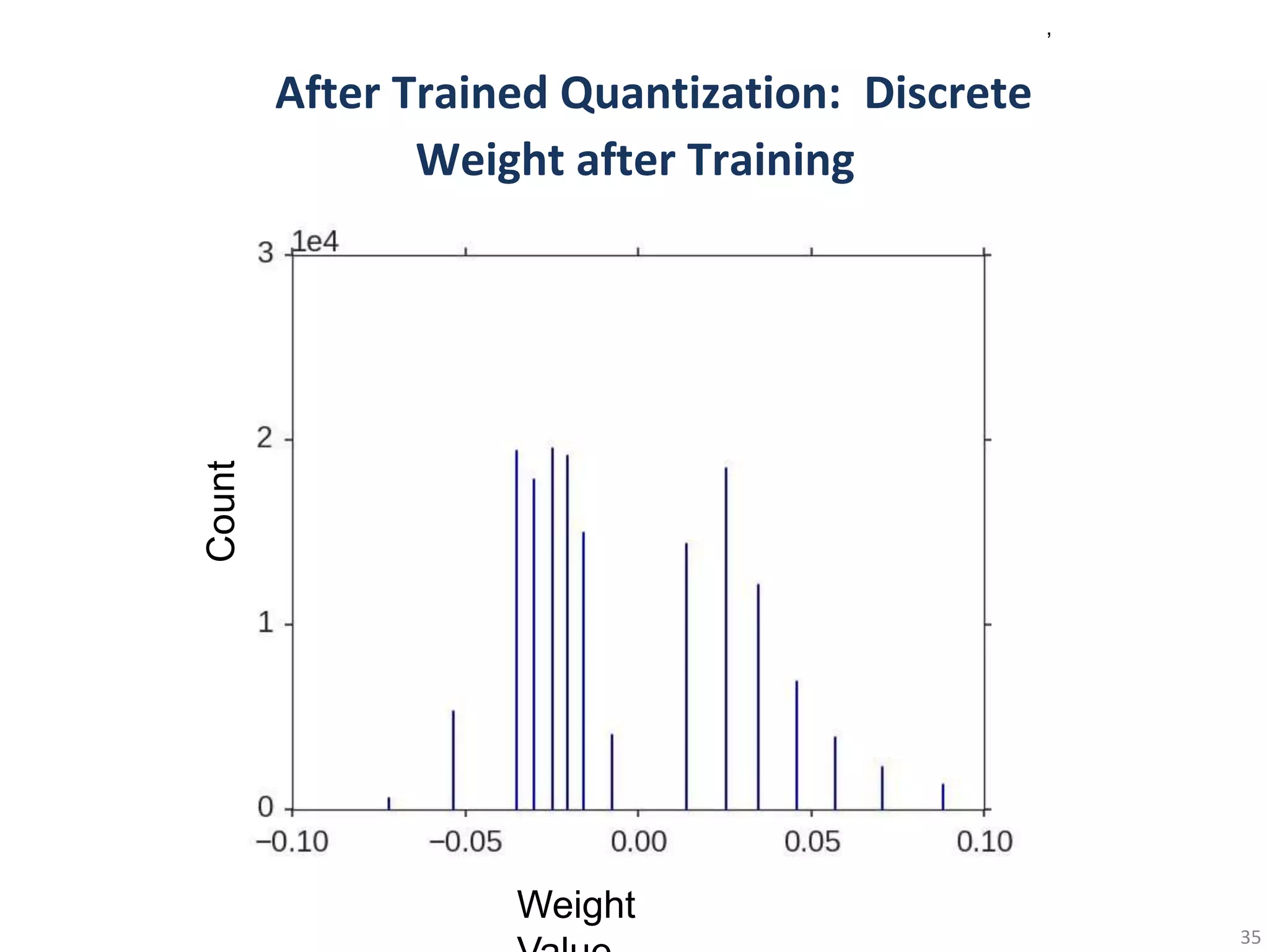
40. •In-frequent weights: use more bits to represent
•Frequent weights: use less bits to represent
,
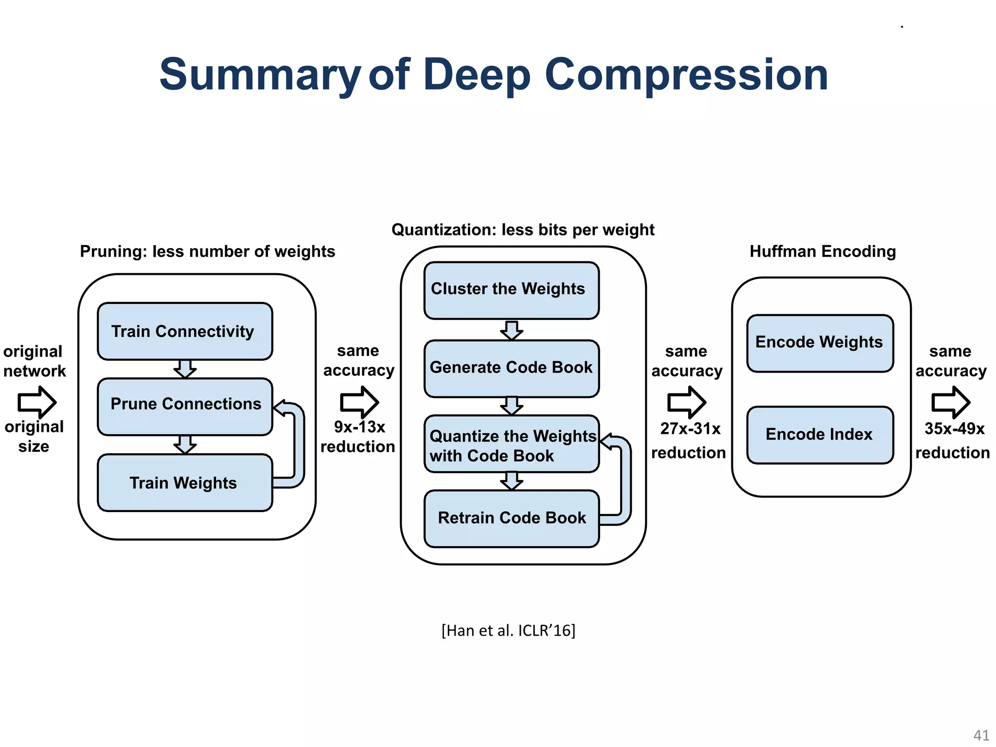
Encode Weights
Encode Index
Huffman Encoding

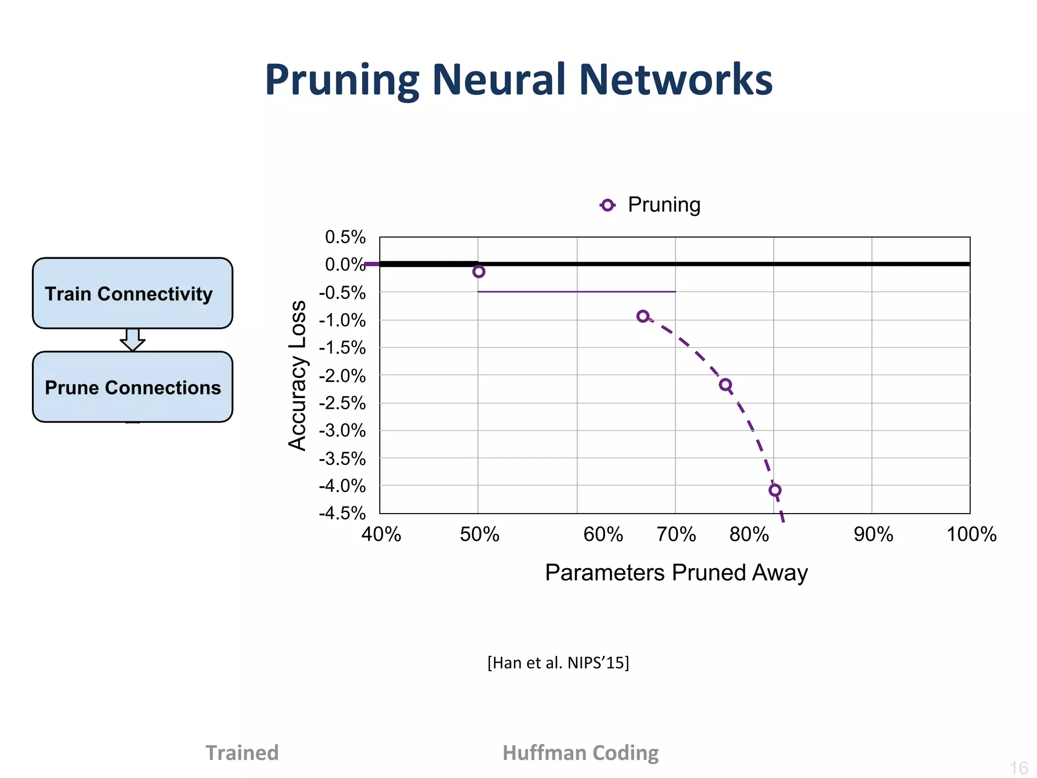
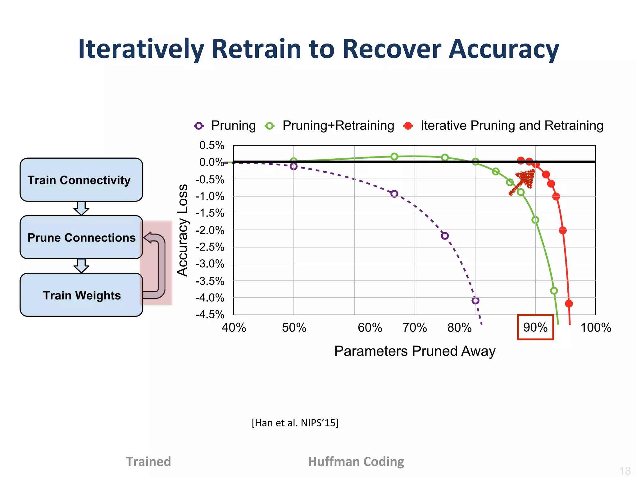
41. Train Connectivity
Prune Connections
Train Weights
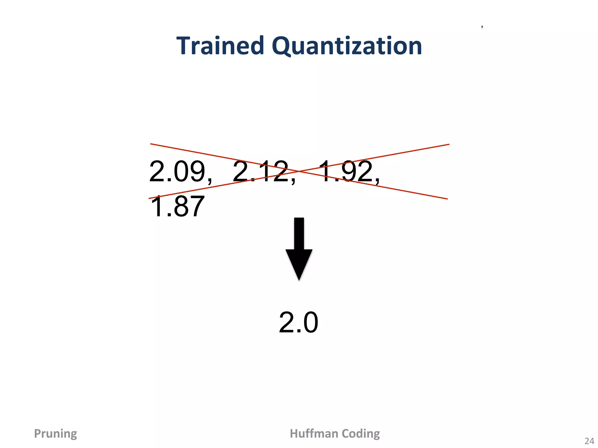
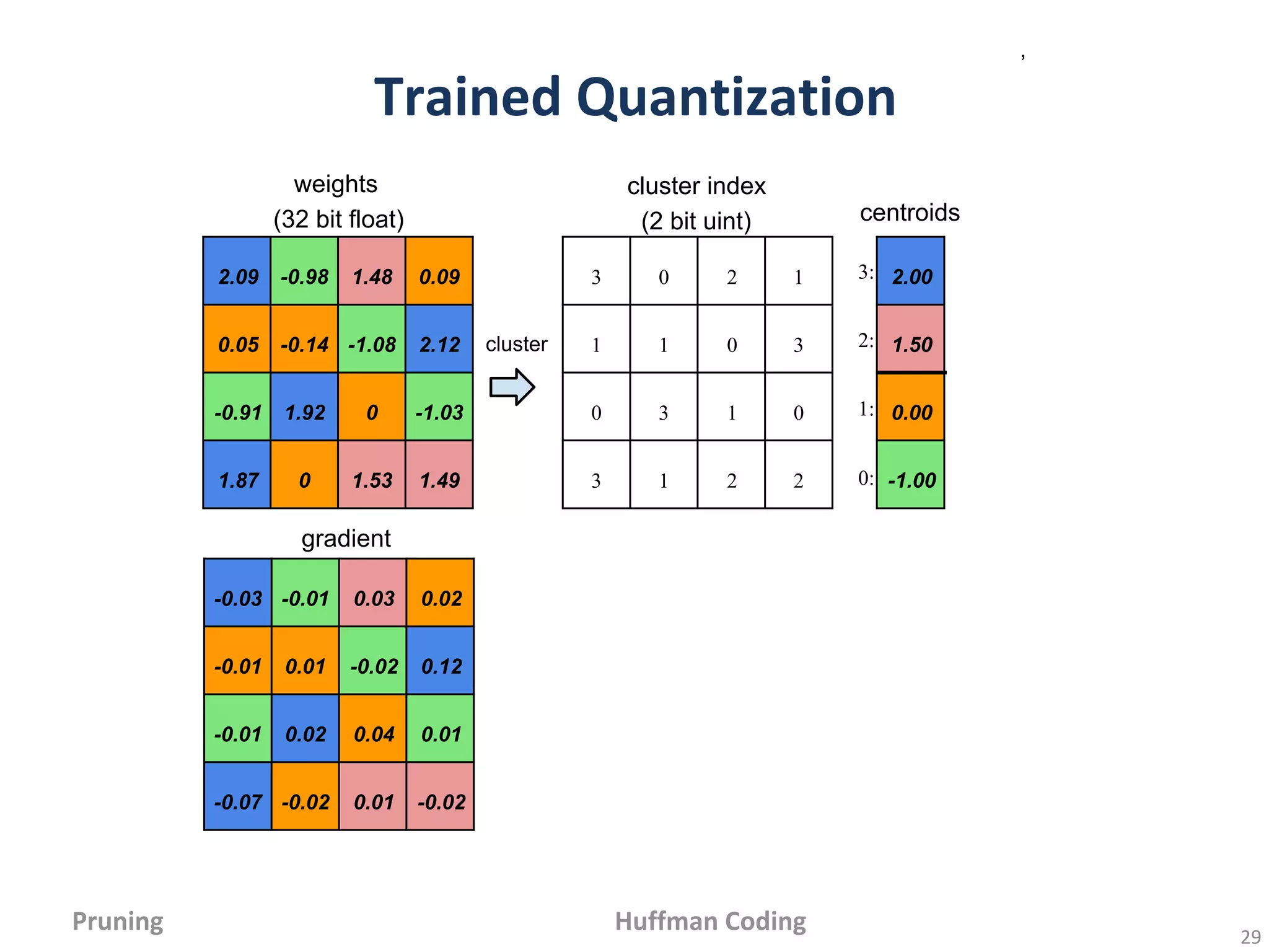
Cluster the Weights
Generate Code Book
Quantize the Weights
with Code Book
Retrain Code Book
Pruning: less number of weights
Quantization: less bits per weight
original
size
9x-13x
reduction
27x-31x
reduction
same
accuracy
same
accuracy
original
network
Encode Weights
Encode Index
Huffman Encoding
35x-49x
reduction
same
accuracy
Summaryof Deep Compression

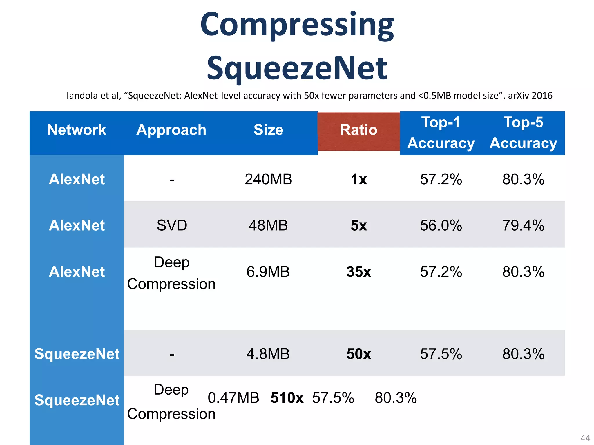
42. Network
Original
Size
Original
Accuracy
Compressed
Accuracy
LeNet-300 1070KB 98.36% 98.42%
LeNet-5 1720KB 99.20% 99.26%
AlexNet 240MB 80.27% 80.30%
VGGNet 550MB 88.68% 89.09%
GoogleNet 28MB 88.90% 88.92%
ResNet-18 44.6MB
Compressed
Compression Size
Ratio
27KB 40x
44KB 39x
6.9MB 35x
11.3MB 49x
2.8MB 10x
4.0MB 11x
89.24% 89.28%
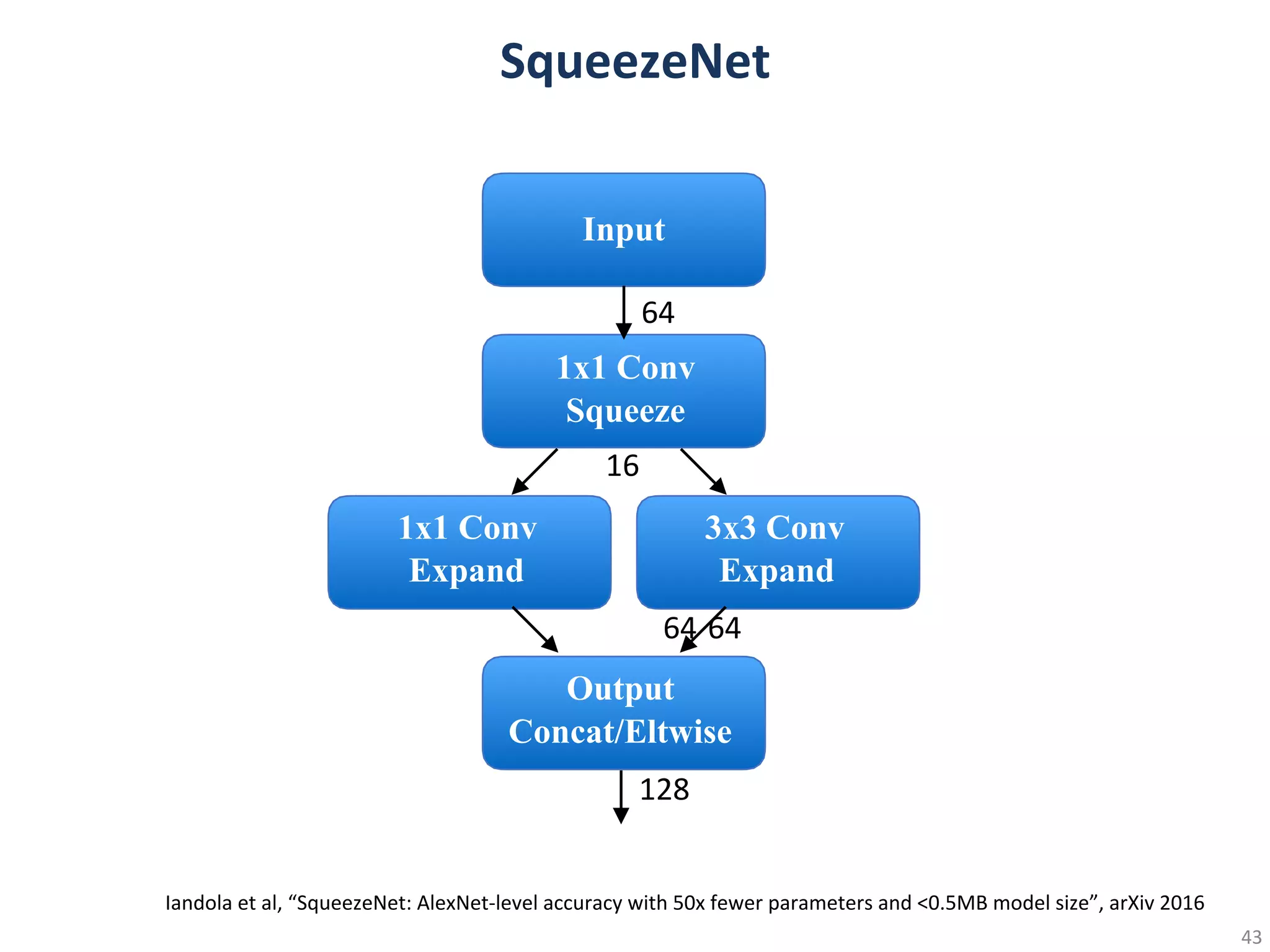
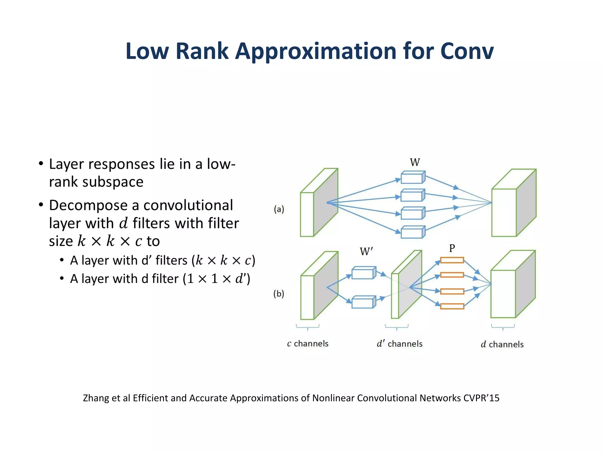
Can we make compact models to begin with?
.

43. 1x1 Conv
Expand
3x3 Conv
Expand
Input
1x1 Conv
Squeeze
Output
Concat/Eltwise

44. Accuracy Accuracy
AlexNet - 240MB 1x 57.2% 80.3%
AlexNet SVD 48MB 5x 56.0% 79.4%
AlexNet
Deep
Compression
6.9MB 35x 57.2% 80.3%
SqueezeNet - 4.8MB 50x 57.5% 80.3%
SqueezeNet
Deep
0.47MB 510x 57.5% 80.3%
Compression
Network Approach Size Ratio
Top-1 Top-5

45. Average
CPU GPU mGPU
0.6x

46. Average
CPU GPU mGPU

47. Deep
Compression
F
8

48. • 1. Pruning
• 2. Weight Sharing
• 3. Quantization
• 4. Low Rank
Approximation
• 5. Binary / Ternary Net
• 6. Winograd
Transformation

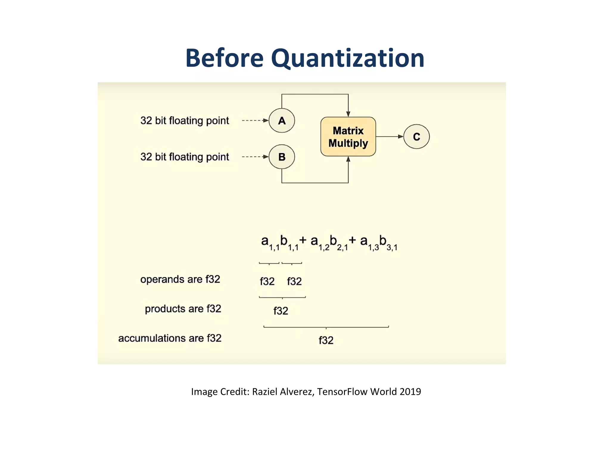
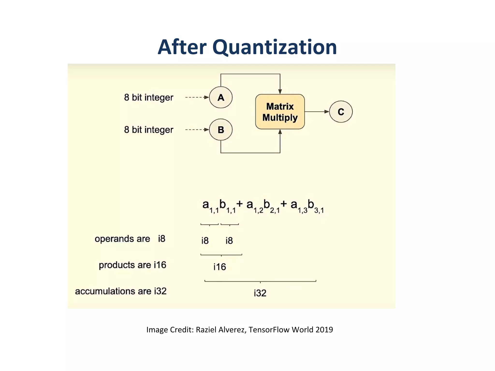
49. •Train with float
•Quantizing the weight and
activation:
• Gather the statistics for
weight and activation
• Choose proper radix point
position
•Fine-tune in float format
•Convert to fixed-point format

53. 1
O.
9
O.
8
O.
7
O.
6
O.
5
O.
4
O.
3
O.
2
O.
1
O
GoogleNet
fp32Fixed 16 Fixed 8 Fixed6
1
O.
9
O.
8
O.
7
O.
6
O.
5
O.
4
O.
3
O.
2
O.
1
O
VGG-16
fp32Fixed 16 Fixed 8 Fixed 6

54. • 1. Pruning
• 2. Weight Sharing
• 3. Quantization
• 4. Low Rank
Approximation
• 5. Binary / Ternary Net
• 6. Winograd
Transformation

57. • 1. Pruning
• 2. Weight Sharing
• 3. Quantization
• 4. Low Rank
Approximation
• 5. Binary / Ternary Net
• 6. Winograd
Transformation

58. -1 0 1−0.05 0.05
0
1600
3200
6400
4800
0
Weight Value
Count
=>

59. Normalize
-1 1
Quantize
-1 0 1 -1 0 1 Wp-t 0
t
Loss
Scale
Wn Wp
Feed Forward Back Propagate Inference Time
Trained
Quantization
-Wn 0
Full Precision Weight
Normalized
Full Precision Weight
Final Ternary WeightIntermediate Ternary Weight
gradient1 gradient2

60. TernaryWeightValue
3
2
1
0
-1
-2
-3
res1.0/conv1/Wn res1.0/conv1/Wp linear/Wn linear/Wpres3.2/conv2/Wn res3.2/conv2/Wp
TernaryWeight
Percentage
100%
75%
50%
25%
0%
0 50 100
Negatives Zeros Positives
Epochs
150 0 50 100
Negatives Zeros Positives
150 0 50 100 150
Negatives Zeros Positives
Ternary weights value (above) and distribution (below) with iterations for different
layers of ResNet-20 on CIFAR-10.

61. • 1. Pruning
• 2. Weight Sharing
• 3. Quantization
• 4. Low Rank
Approximation
• 5. Binary / Ternary Net
• 6. Winograd
Transformation

62. Compute Bound
8 7 6
5 4 3
2 1 0
Filter
0 1 2
3 4 5
6 7 8
Image
Tensor
6 2 8 07 1
0 8 1 7 2 6
4 4 5 33 5
9xC FMAs/Output: Math Intensive
4 0 4 1 4 2
4 3 4 4 4 5
4 6 4 7 4 8
9xK FMAs/Input: Good Data Reuse
∑
✽
Direct convolution: we need 9xCx4 = 36xC FMAs for 4 outputs

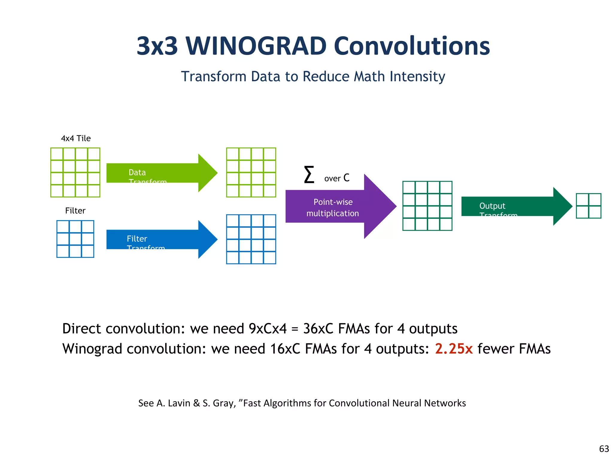
63. Transform Data to Reduce Math Intensity
4x4 Tile
Output
Transform
Filter
Data
Transform
Filter
Transform
∑ over C
Point-wise
multiplication
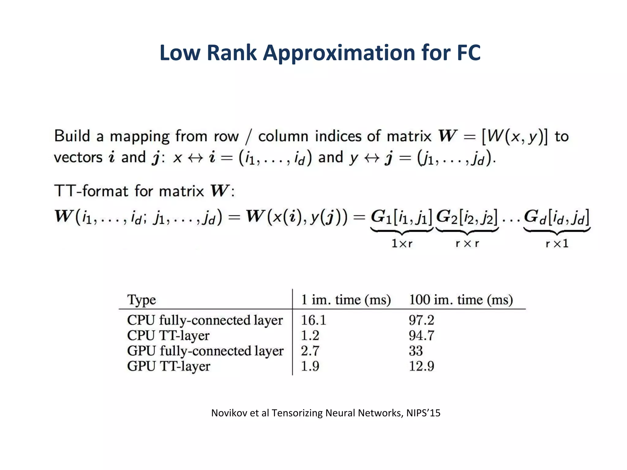
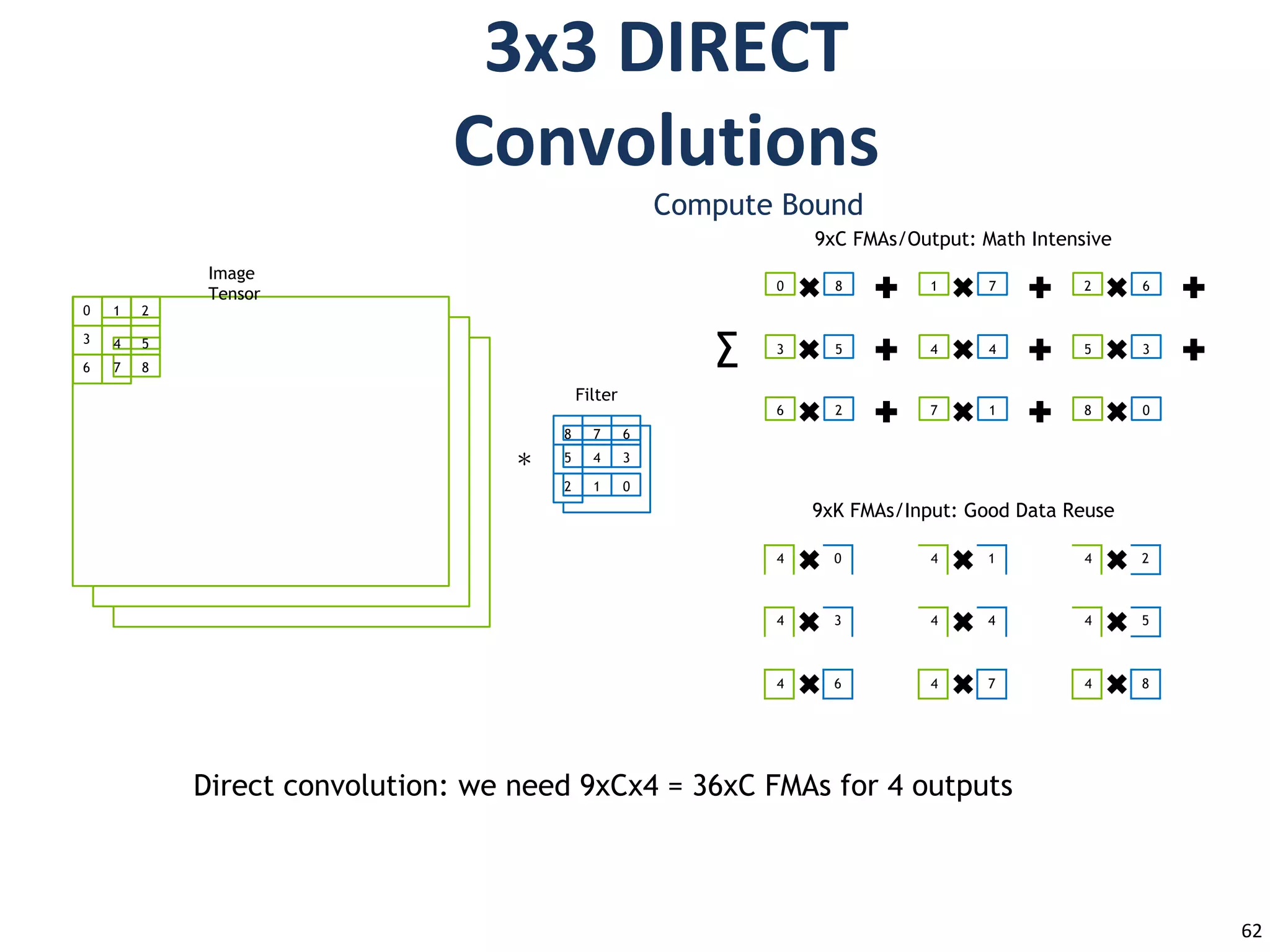
Direct convolution: we need 9xCx4 = 36xC FMAs for 4 outputs
Winograd convolution: we need 16xC FMAs for 4 outputs: 2.25x fewer FMAs

64. VGG16, Batch Size 1 – Relative
Performance
2.00
1.50
1.00
0.50
0.00 conv 1.1 conv 1.2 conv 2.1 conv 2.2 conv 3.1 conv 3.2 conv 4.1 conv 4.2 conv 5.0
cuDNN 3 cuDNN 5

65. •

71. 1.
2.
3.
4.
5.

72. •
1.
2.
•
1.
2.

74. 74

75. darshancganji12@gmal.com