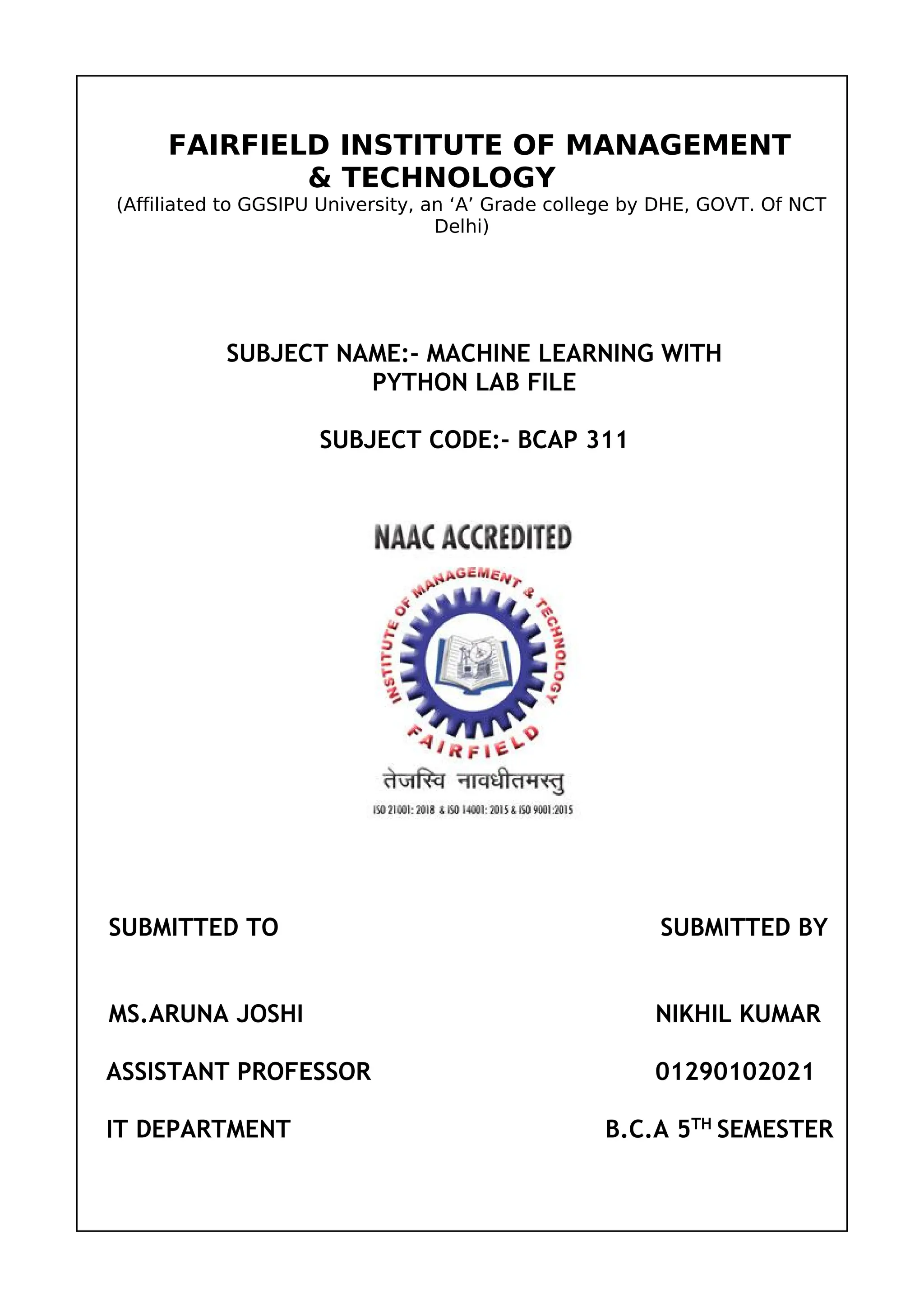
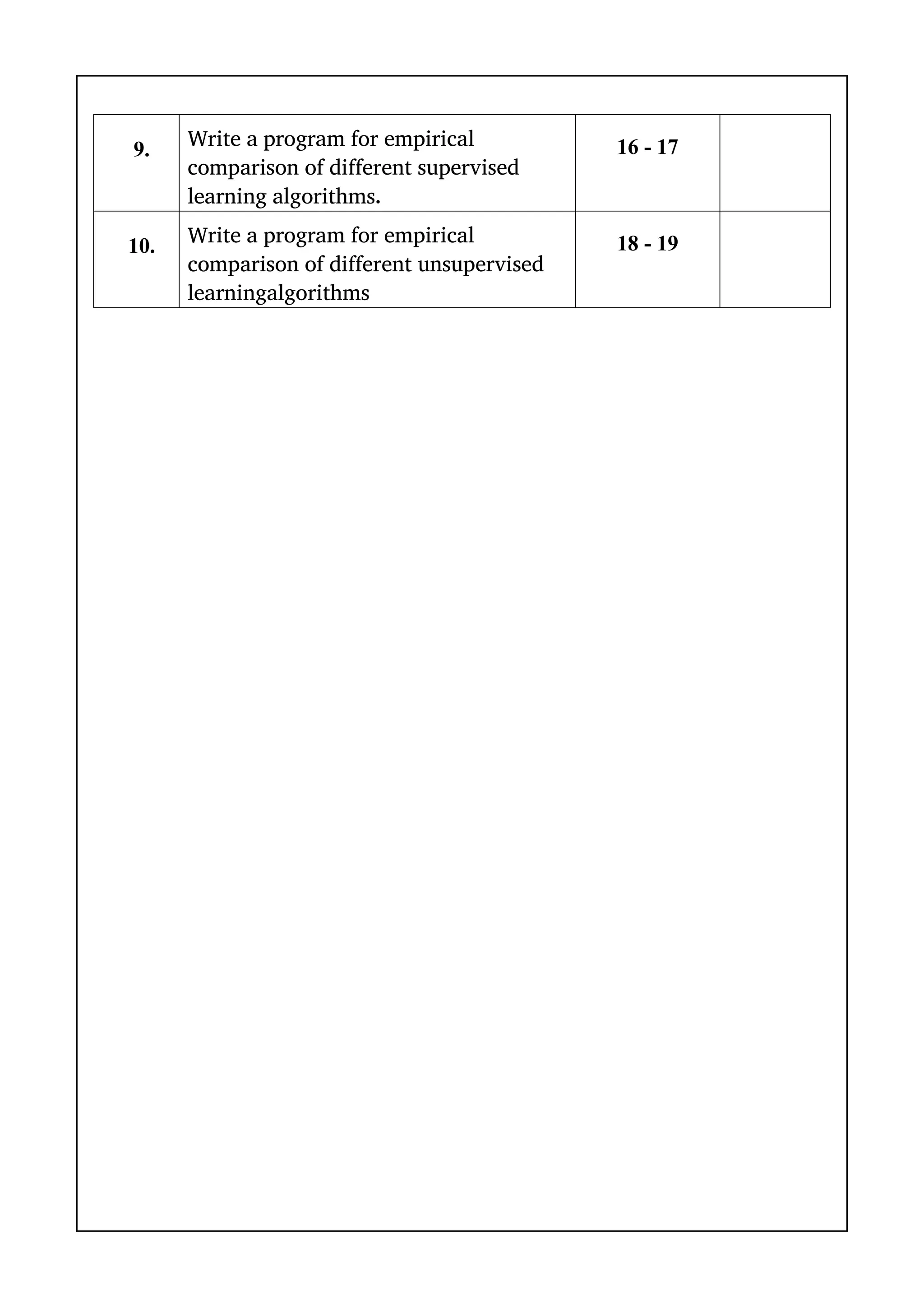
1) The document provides a list of 10 practical machine learning experiments to implement using Python. 2) The experiments include implementing algorithms such as linear regression, logistic regression, KNN, random forest, neural networks, K-means clustering, and comparing the performance of different supervised and unsupervised learning models. 3) The code snippets provided show how to apply these algorithms to sample datasets, calculate accuracy scores, and visualize the results.

1. FAIRFIELD INSTITUTE OF MANAGEMENT
& TECHNOLOGY
(Affiliated to GGSIPU University, an ‘A’ Grade college by DHE, GOVT. Of NCT
Delhi)
SUBJECT NAME:- MACHINE LEARNING WITH
PYTHON LAB FILE
SUBJECT CODE:- BCAP 311
SUBMITTED TO SUBMITTED BY
MS.ARUNA JOSHI NIKHIL KUMAR
ASSISTANT PROFESSOR 01290102021
IT DEPARTMENT B.C.A 5TH
SEMESTER

2. LIST OF PRACTICALS
S.NO PRACTICALS PAGE NO. T.SIGN
1. Extract the data from the database
using python.
1
2. Write a program to implement linear
and logistic regression.
2 - 4
3.
Write a program to implement the
naïve Bayesian classifier for a sample
training data set stored as a .CSV file.
Compute the accuracy of the classifier,
considering few test data sets.
5 - 6
4. Write a program to implement k-
nearest neighbors (KNN) and Support
Vector Machine (SVM) Algorithm for
classification.
7 - 8
5. Implement classification of a given
dataset using random forest.
9
6.
Build an Artificial Neural Network
(ANN) by implementing the Back
propagation algorithm and test the
same using appropriate data sets.
10 - 11
7.
Apply k-Means algorithm k-Means
algorithm to cluster a set of data stored
in a. CSV file. Use the same data set for
clustering using the k-Means
algorithm.
Compare the results of these two
algorithms and comment on the quality
of clustering. You can add Python ML
library classes in the program.
12 - 13
8. Write a program to implement Self -
Organizing Map (SOM).
14 - 15

3. 9. Write a program for empirical
comparison of different supervised
learning algorithms.
16 - 17
10. Write a program for empirical
comparison of different unsupervised
learningalgorithms
18 - 19

4. 1
1) Extract the data from the database using python.
this is our data in SampleDB database now we will write a code fro extract the data using python.
CODE:-
import mysql.connector
myconn = mysql.connector.connect(host = "localhost",
user = "root",passwd = "test",database="SampleDB")
cur = myconn.cursor()
cur.execute("select * from STUDENTS")
result = cur.fetchall()
print("Student Details are :")
for x in result:
print(x)
myconn.commit()
myconn.close()
OUTPUT:-

5. 2
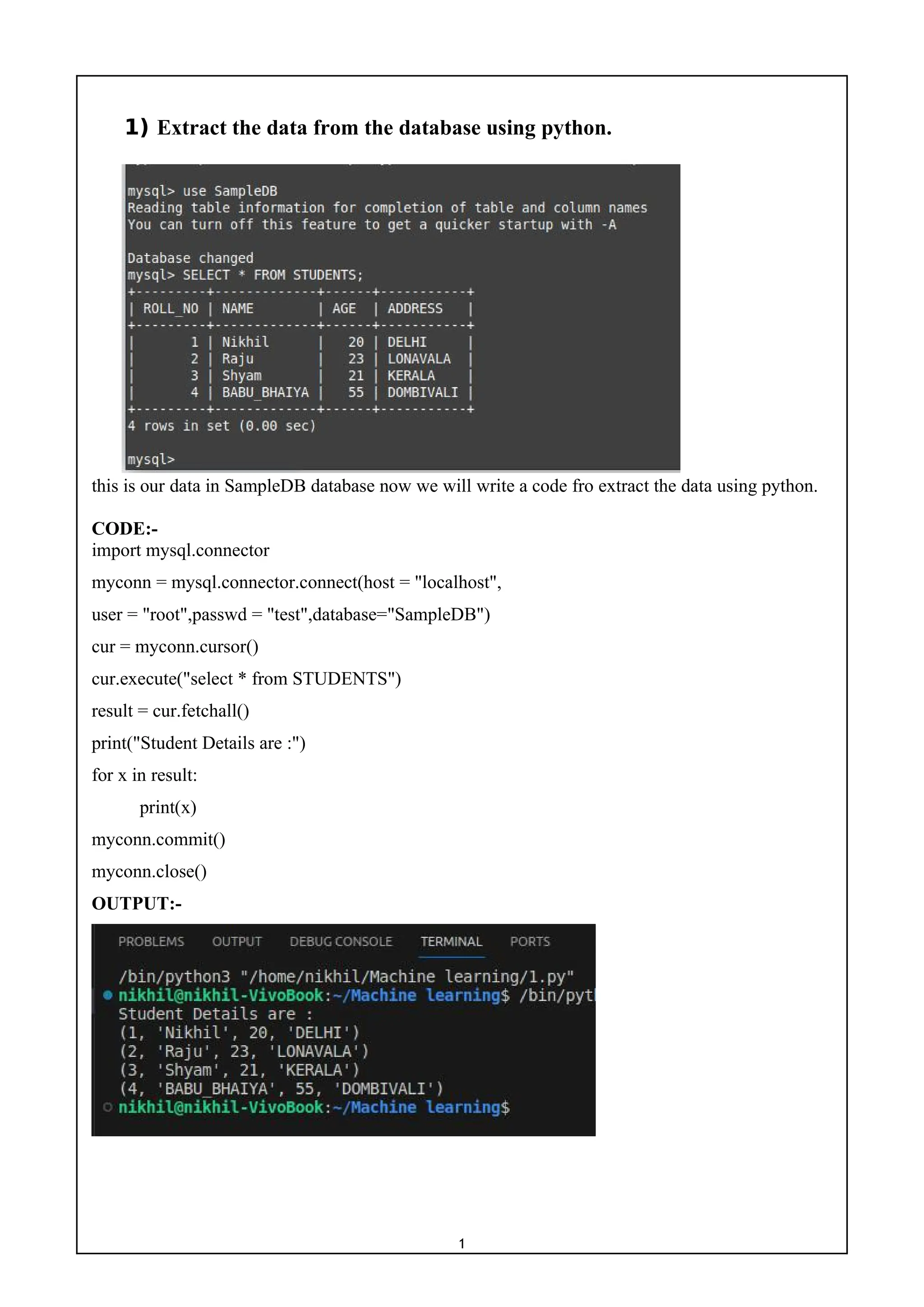
2) Write a program to implement linear and logistic regression.
a) Linear regression:-
import numpy as nmp
import matplotlib.pyplot as mtplt
def estimate_coeff(p, q):
n1 = nmp.size(p)
m_p = nmp.mean(p)
m_q = nmp.mean(q)
SS_pq = nmp.sum(q * p) - n1 * m_q * m_p
SS_pp = nmp.sum(p * p) - n1 * m_p * m_p
b_1 = SS_pq / SS_pp
b_0 = m_q - b_1 * m_p
return (b_0, b_1)
def plot_regression_line(p, q, b):
mtplt.scatter(p, q, color = "m",
marker = "o", s = 30)
q_pred = b[0] + b[1] * p
mtplt.plot(p, q_pred, color = "g")
mtplt.xlabel('p')
mtplt.ylabel('q')
mtplt.show()
def main():
p = nmp.array([10, 11, 12, 13, 14, 15, 16, 17, 18, 19])
q = nmp.array([11, 13, 12, 15, 17, 18, 18, 19, 20, 22])
b = estimate_coeff(p, q)
print("Estimated coefficients are :nb_0 = {}
nb_1 = {}".format(b[0], b[1]))
plot_regression_line(p, q, b)
if __name__ == "__main__":
main()

6. 3
OUTPUT:-

7. 4
b) Logistic regression:-
Now we have a logistic regression object that is ready to whether a tumor is cancerous
based on the tumor size:
CODE:-
import numpy
from sklearn import linear_model
X = numpy.array([3.78, 2.44, 2.09, 0.14, 1.72, 1.65, 4.92, 4.37, 4.96, 4.52, 3.69,
5.88]).reshape(-1,1)
y = numpy.array([0, 0, 0, 0, 0, 0, 1, 1, 1, 1, 1, 1])
logr = linear_model.LogisticRegression()
logr.fit(X,y)
print(predicted)
OUTPUT:-
We have predicted that a tumor with a size of 3.46mm will not be cancerous.

8. 5
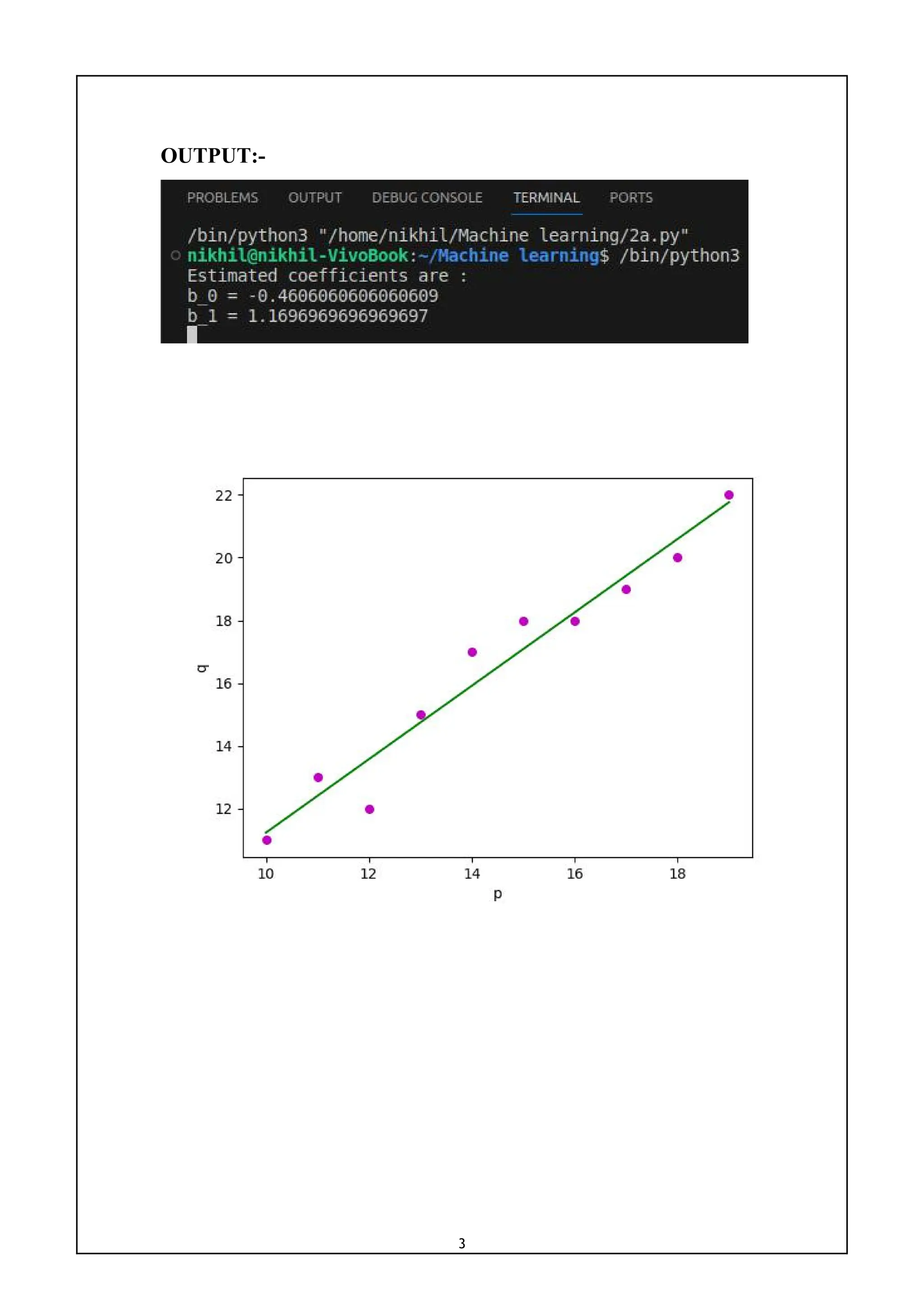
3) Write a program to implement the naïve Bayesian classifier for a sample
training data set stored as a .CSV file. Compute the accuracy of the classifier,
considering few test data sets.
CODE:-
import pandas as pd
from sklearn import tree
from sklearn.preprocessing import LabelEncoder
from sklearn.naive_bayes import GaussianNB
data = pd.read_csv('tennisdata.csv')
print("The first 5 values of data is :n",data.head())
X = data.iloc[:,:-1]
print("nThe First 5 values of train data isn",X.head())
y = data.iloc[:,-1]
print("nThe first 5 values of Train output isn",y.head())
le_outlook = LabelEncoder()
X.Outlook = le_outlook.fit_transform(X.Outlook)
le_Temperature = LabelEncoder()
X.Temperature = le_Temperature.fit_transform(X.Temperature)
le_Humidity = LabelEncoder()
X.Humidity = le_Humidity.fit_transform(X.Humidity)
le_Windy = LabelEncoder()
X.Windy = le_Windy.fit_transform(X.Windy)
print("nNow the Train data is :n",X.head())
le_PlayTennis = LabelEncoder()
y = le_PlayTennis.fit_transform(y)
print("nNow the Train output isn",y)
from sklearn.model_selection import train_test_split
X_train, X_test, y_train, y_test = train_test_split(X,y, test_size=0.20)
classifier = GaussianNB()
classifier.fit(X_train,y_train)
from sklearn.metrics import accuracy_score
print("Accuracy is:",accuracy_score(classifier.predict(X_test),y_test))

9. 6
OUTPUT:-

10. 7
4) Write a program to implement k-nearest neighbors (KNN) and Support
Vector Machine (SVM) Algorithm for classification.
CODE:-
from sklearn.model_selection import train_test_split
from sklearn.neighbors import KNeighborsClassifier
from sklearn import svm
from sklearn import datasets
from sklearn.metrics import accuracy_score
# Load the Iris dataset
iris = datasets.load_iris()
X = iris.data
y = iris.target
X_train, X_test, y_train, y_test = train_test_split(X, y, test_size=0.2, random_state=42)
# K-Nearest Neighbors (KNN) classifier
def knn_classifier(X_train, y_train, X_test, k):
knn = KNeighborsClassifier(n_neighbors=k)
knn.fit(X_train, y_train)
predictions = knn.predict(X_test)
return predictions
# Support Vector Machine (SVM) classifier
def svm_classifier(X_train, y_train, X_test):
svm_model = svm.SVC()
svm_model.fit(X_train, y_train)
predictions = svm_model.predict(X_test)
return predictions
k_value = 7
# Make predictions using KNN
knn_predictions = knn_classifier(X_train, y_train, X_test, k_value)
# Make predictions using SVM
svm_predictions = svm_classifier(X_train, y_train, X_test)
knn_accuracy = accuracy_score(y_test, knn_predictions)
svm_accuracy = accuracy_score(y_test, svm_predictions)
print(“ ”)
print(f"K-Nearest Neighbors (KNN) Accuracy: {knn_accuracy:.2f}")

11. 8
print(“ ”)
print(f"Support Vector Machine (SVM) Accuracy: {svm_accuracy:.2f}")
OUTPUT:-

12. 9
5) Implement classification of a given dataset using random forest.
CODE:-
from sklearn.model_selection import train_test_split
from sklearn.ensemble import RandomForestClassifier
from sklearn import datasets
from sklearn.metrics import accuracy_score
iris = datasets.load_iris()
X = iris.data
y = iris.target
X_train, X_test, y_train, y_test = train_test_split(X, y, test_size=0.2, random_state=42)
def random_forest_classifier(X_train, y_train, X_test, n_estimators):
rf_model = RandomForestClassifier(n_estimators=n_estimators, random_state=42)
rf_model.fit(X_train, y_train)
predictions = rf_model.predict(X_test)
return predictions
num_trees = 34
rf_predictions = random_forest_classifier(X_train, y_train, X_test, num_trees)
rf_accuracy = accuracy_score(y_test, rf_predictions)
print(f"Random Forest Accuracy: {rf_accuracy:.2f}")
OUTPUT:-

13. 10
6) Build an Artificial Neural Network (ANN) by implementing the Back
propagation algorithm and test the same using appropriate data sets.
CODE:-
import numpy as np
def sigmoid(x):
return 1 / (1 + np.exp(-x))
def sigmoid_derivative(x):
return x * (1 - x)
def initialize_weights(input_size, hidden_size, output_size):
input_hidden_weights = 2 * np.random.rand(input_size, hidden_size) - 1
hidden_output_weights = 2 * np.random.rand(hidden_size, output_size) - 1
return input_hidden_weights, hidden_output_weights
def train_neural_network(X, y, epochs, learning_rate):
input_size = X.shape[1]
hidden_size = 3
output_size = 1
input_hidden_weights, hidden_output_weights = initialize_weights(input_size, hidden_size,
output_size)
for epoch in range(epochs):
hidden_layer_input = np.dot(X, input_hidden_weights)
hidden_layer_output = sigmoid(hidden_layer_input)
output_layer_input = np.dot(hidden_layer_output, hidden_output_weights)
predicted_output = sigmoid(output_layer_input)
error = y - predicted_output
output_error = error * sigmoid_derivative(predicted_output)
hidden_layer_error = output_error.dot(hidden_output_weights.T) *
sigmoid_derivative(hidden_layer_output)
hidden_output_weights += hidden_layer_output.T.dot(output_error) * learning_rate
input_hidden_weights += X.T.dot(hidden_layer_error) * learning_rate
if epoch % 1000 == 0:
print(f'Epoch {epoch}, Loss: {np.mean(np.abs(error))}')

14. 11
return input_hidden_weights, hidden_output_weights
X = np.array([[0, 0], [0, 1], [1, 0], [1, 1]])
y = np.array([[0], [1], [1], [1]])
epochs = 10000
learning_rate = 0.1
trained_input_hidden_weights,trained_hidden_output_weights = train_neural_network(X, y,
epochs, learning_rate)
hidden_layer_output = sigmoid(np.dot(X, trained_input_hidden_weights))
predicted_output=sigmoid(np.dot(hidden_layer_output, trained_hidden_output_weights))
print("Predicted Output:")
print(predicted_output)
OUTPUT:-

15. 12
7) Apply k-Means algorithm k-Means algorithm to cluster a set of data
stored in a .CSV file. Use the same data set for clustering using the k-Means
algorithm. Compare the results of these two algorithms and comment on the
quality of clustering. You can add Python ML library classes in the program.
CODE:-
import matplotlib.pyplot as plt
from sklearn import datasets
from sklearn.cluster import KMeans
import sklearn.metrics as sm
import pandas as pd
import numpy as np
iris = datasets.load_iris()
X = pd.DataFrame(iris.data)
X.columns = ['Sepal_Length','Sepal_Width','Petal_Length','Petal_Width']
y = pd.DataFrame(iris.target)
y.columns = ['Targets']
model = KMeans(n_clusters=3)
model.fit(X)
plt.figure(figsize=(14,7))
colormap = np.array(['red', 'lime', 'black'])
plt.subplot(1, 2, 1)
plt.scatter(X.Petal_Length, X.Petal_Width, c=colormap[y.Targets], s=40)
plt.title('Real Classification')
plt.xlabel('Petal Length')
plt.ylabel('Petal Width')
# Plot the Models Classifications
plt.subplot(1, 2, 2)
plt.scatter(X.Petal_Length, X.Petal_Width, c=colormap[model.labels_], s=40)
plt.title('K Mean Classification')
plt.xlabel('Petal Length')
plt.ylabel('Petal Width')
print(“ ”)
print('The accuracy score of K-Mean: ',sm.accuracy_score(y, model.labels_))

16. 13
print('The Confusion matrixof K-Mean: ',sm.confusion_matrix(y, model.labels_))
from sklearn import preprocessing
scaler = preprocessing.StandardScaler()
scaler.fit(X)
xsa = scaler.transform(X)
xs = pd.DataFrame(xsa, columns = X.columns)
from sklearn.mixture import GaussianMixture
gmm = GaussianMixture(n_components=3)
gmm.fit(xs)
y_gmm = gmm.predict(xs)
#y_cluster_gmm
plt.subplot(2, 2, 3)
plt.scatter(X.Petal_Length, X.Petal_Width, c=colormap[y_gmm], s=40)
plt.title('GMM Classification')
plt.xlabel('Petal Length')
plt.ylabel('Petal Width')
print("")
print('The accuracy score of EM: ',sm.accuracy_score(y, y_gmm))
print('The Confusion matrix of EM: ',sm.confusion_matrix(y, y_gmm))
OUTPUT:-

17. 14
8) Write a program to implement Self - Organizing Map (SOM).
CODE:-
import numpy as np
import matplotlib.pyplot as plt
class SelfOrganizingMap:
def __init__(self, input_size, map_size):
self.input_size = input_size
self.map_size = map_size
self.weights = np.random.rand(map_size[0], map_size[1], input_size)
def find_best_matching_unit(self, input_vector):
distances = np.linalg.norm(self.weights - input_vector, axis=-1)
bmu_index = np.unravel_index(np.argmin(distances), distances.shape)
return bmu_index
def update_weights(self, input_vector, bmu_index, learning_rate, radius):
for i in range(self.map_size[0]):
for j in range(self.map_size[1]):
distance = np.linalg.norm(np.array([i, j]) - np.array(bmu_index))
if distance <= radius:
influence = np.exp(-(distance ** 2) / (2 * radius ** 2))
self.weights[i, j, :] += learning_rate * influence * (input_vector - self.weights[i, j, :])
def train(self, data, epochs=100, initial_learning_rate=0.1, initial_radius=None):
if initial_radius is None:
initial_radius = max(self.map_size) / 2
for epoch in range(epochs):
for input_vector in data:
bmu_index = self.find_best_matching_unit(input_vector)
learning_rate = initial_learning_rate * (1 - epoch/epochs)
radius = initial_radius * np.exp(-epoch/epochs)
self.update_weights(input_vector, bmu_index, learning_rate, radius)
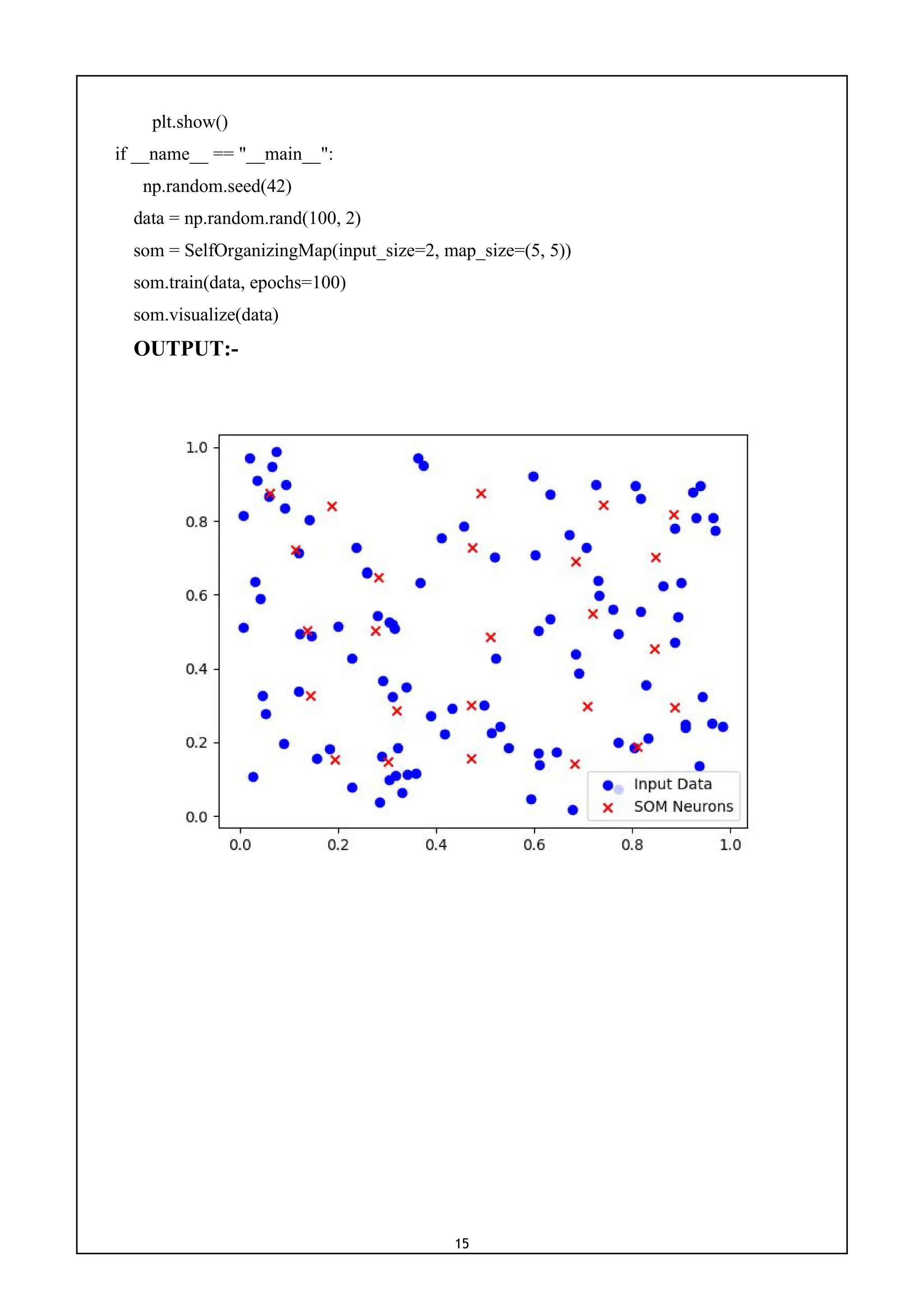
def visualize(self, data):
plt.scatter(data[:, 0], data[:, 1], c='b', marker='o', label='Input Data')
plt.scatter(self.weights[:, :, 0], self.weights[:, :, 1], c='r', marker='x', label='SOM Neurons')
plt.legend()

18. 15
plt.show()
if __name__ == "__main__":
np.random.seed(42)
data = np.random.rand(100, 2)
som = SelfOrganizingMap(input_size=2, map_size=(5, 5))
som.train(data, epochs=100)
som.visualize(data)
OUTPUT:-

19. 16
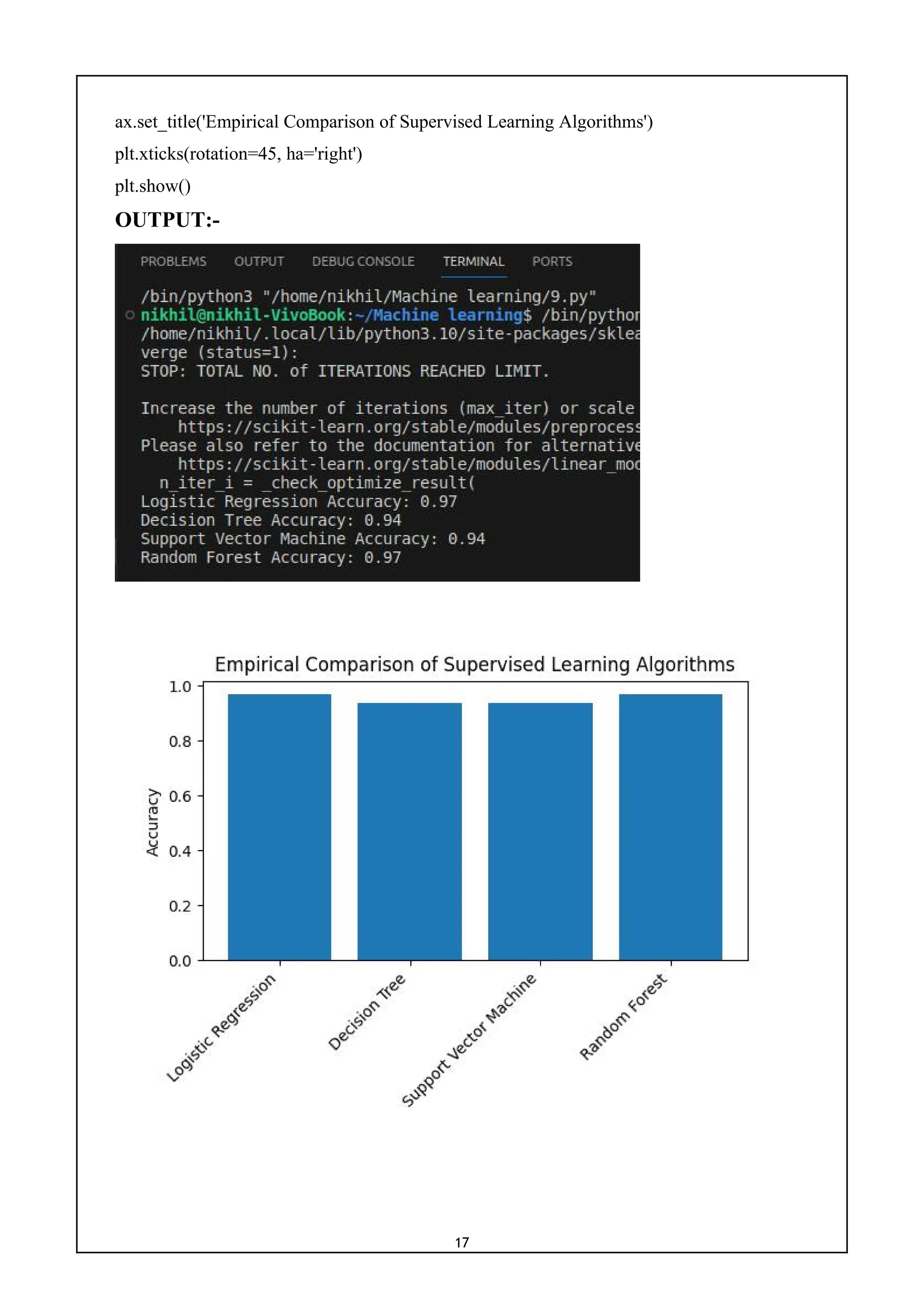
9) Write a program for empirical comparison of different supervised
learning algorithms.
CODE:-
import numpy as np
import matplotlib.pyplot as plt
from sklearn.datasets import load_breast_cancer
from sklearn.model_selection import train_test_split
from sklearn.linear_model import LogisticRegression
from sklearn.tree import DecisionTreeClassifier
from sklearn.svm import SVC
from sklearn.ensemble import RandomForestClassifier
from sklearn.metrics import accuracy_score
cancer = load_breast_cancer()
X, y = cancer.data, cancer.target
X_train, X_test, y_train, y_test = train_test_split(X, y, test_size=0.3, random_state=42)
classifiers = {
'Logistic Regression': LogisticRegression(),
'Decision Tree': DecisionTreeClassifier(),
'Support Vector Machine': SVC(),
'Random Forest': RandomForestClassifier()
}
results = {}
for name, clf in classifiers.items():
clf.fit(X_train, y_train)
y_pred = clf.predict(X_test)
accuracy = accuracy_score(y_test, y_pred)
results[name] = accuracy
print(f'{name} Accuracy: {accuracy:.2f}')
names = list(results.keys())
values = list(results.values())
fig, ax = plt.subplots()
ax.bar(names, values)
ax.set_ylabel('Accuracy')

20. 17
ax.set_title('Empirical Comparison of Supervised Learning Algorithms')
plt.xticks(rotation=45, ha='right')
plt.show()
OUTPUT:-

21. 18
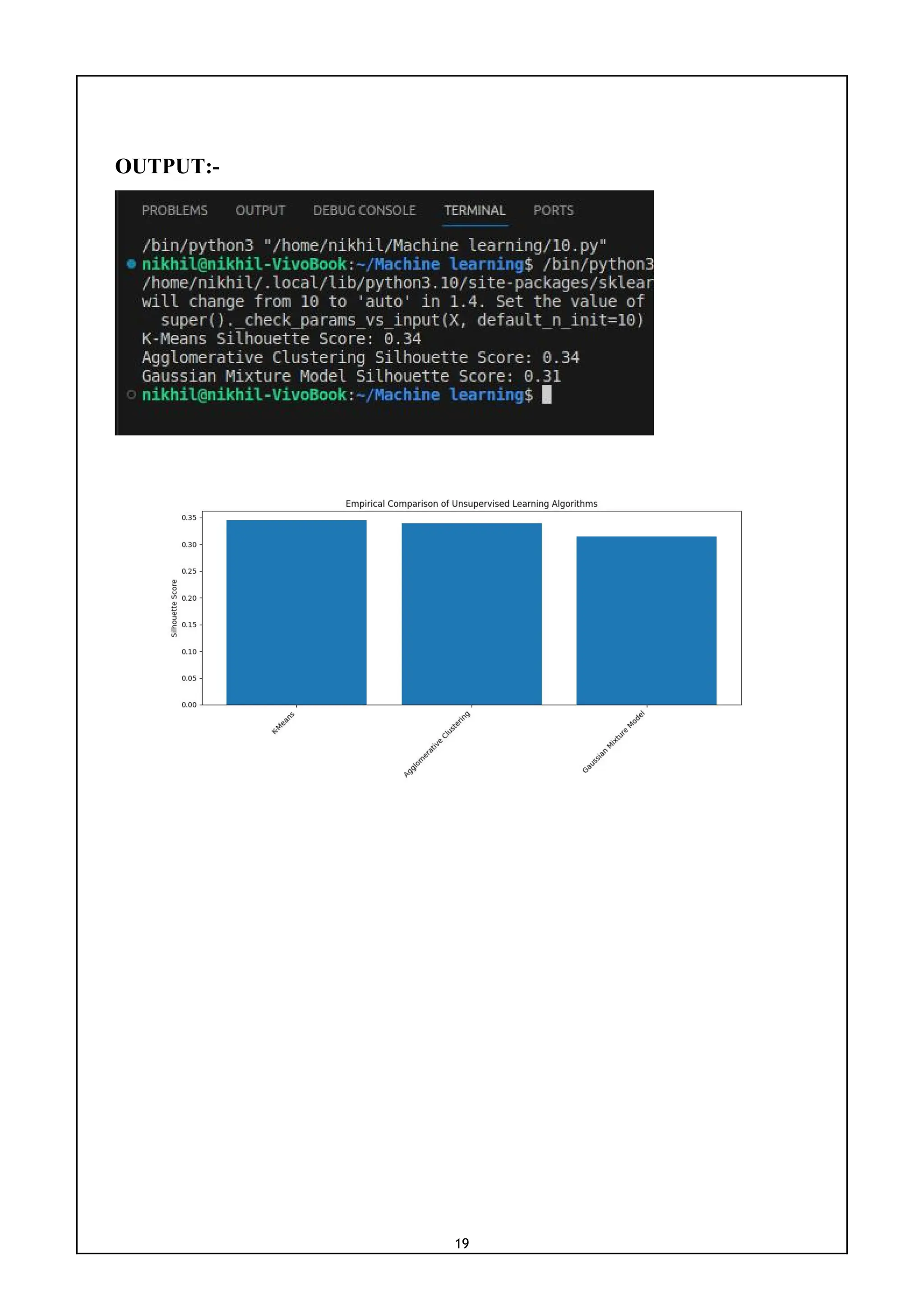
10) Write a program for empirical comparison of different unsupervised
learning algorithms.
CODE:-
import numpy as np
import matplotlib.pyplot as plt
from sklearn.datasets import load_breast_cancer
from sklearn.preprocessing import StandardScaler
from sklearn.cluster import KMeans, AgglomerativeClustering
from sklearn.mixture import GaussianMixture
from sklearn.metrics import silhouette_score
cancer = load_breast_cancer()
X, y = cancer.data, cancer.target
scaler = StandardScaler()
X_scaled = scaler.fit_transform(X)
algorithms = {
'K-Means': KMeans(n_clusters=2),
'Agglomerative Clustering': AgglomerativeClustering(n_clusters=2),
'Gaussian Mixture Model': GaussianMixture(n_components=2)
}
results = {}
for name, algorithm in algorithms.items():
labels = algorithm.fit_predict(X_scaled)
silhouette_avg = silhouette_score(X_scaled, labels)
results[name] = silhouette_avg
print(f'{name} Silhouette Score: {silhouette_avg:.2f}')
names = list(results.keys())
values = list(results.values())
fig, ax = plt.subplots()
ax.bar(names, values)
ax.set_ylabel('Silhouette Score')
ax.set_title('Empirical Comparison of Unsupervised Learning Algorithms')
plt.xticks(rotation=45, ha='right')
plt.show()

22. 19
OUTPUT:-