NAÏVE BAYES
Dr. Amanpreet Kaur​
Associate Professor,
Chitkara University, Punjab
AGENDA - TYPES OF NAÏVE BAYES
CLASSIFIERS
There are three types of classifiers.
They are
• Gaussian Naïve Bayes
• Multinomial Naïve Bayes
• Bernoulli Naïve Bayes
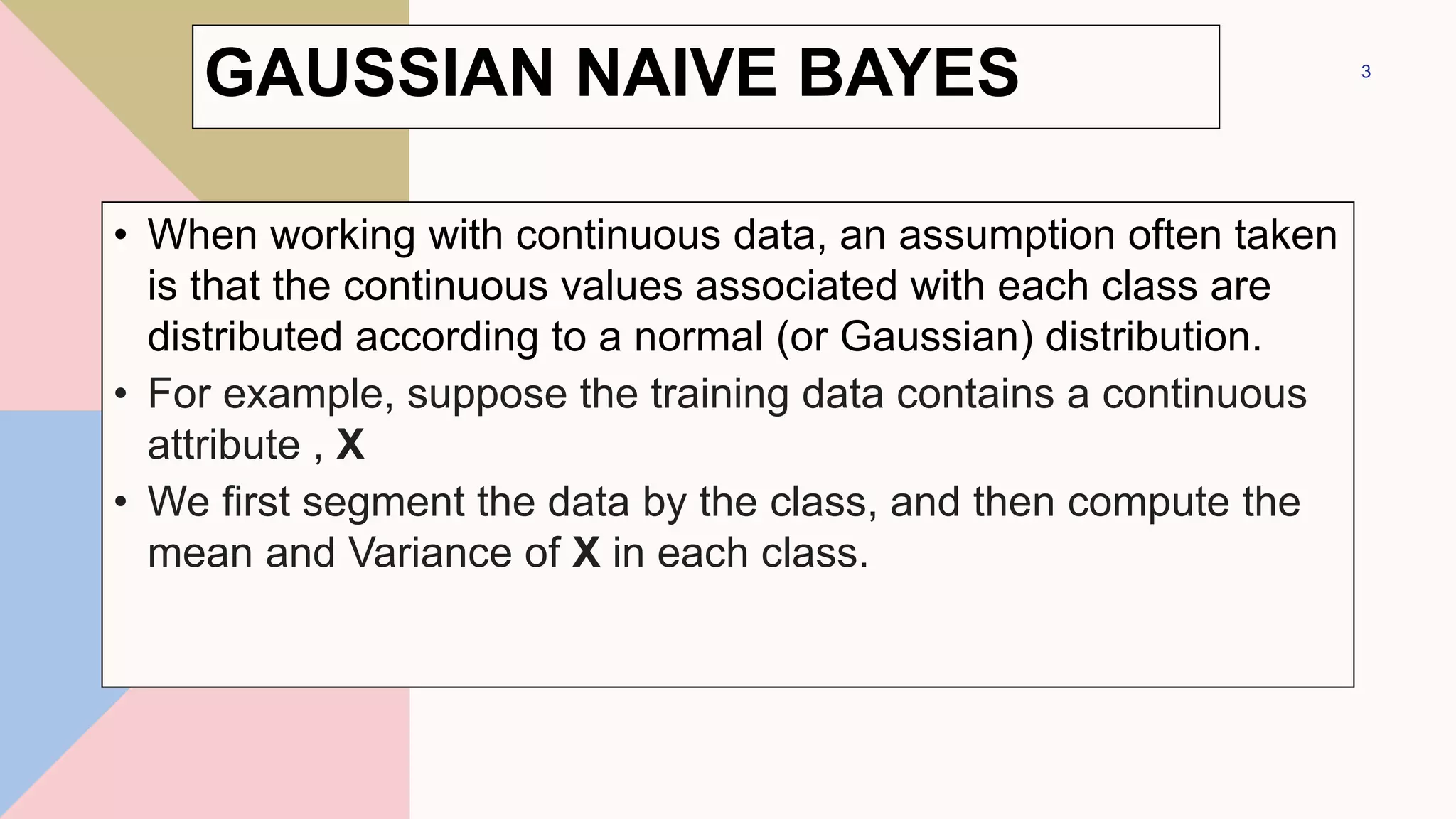
• When working with continuous data, an assumption often taken
is that the continuous values associated with each class are
distributed according to a normal (or Gaussian) distribution.
• For example, suppose the training data contains a continuous
attribute , X
• We first segment the data by the class, and then compute the
mean and Variance of X in each class.
3
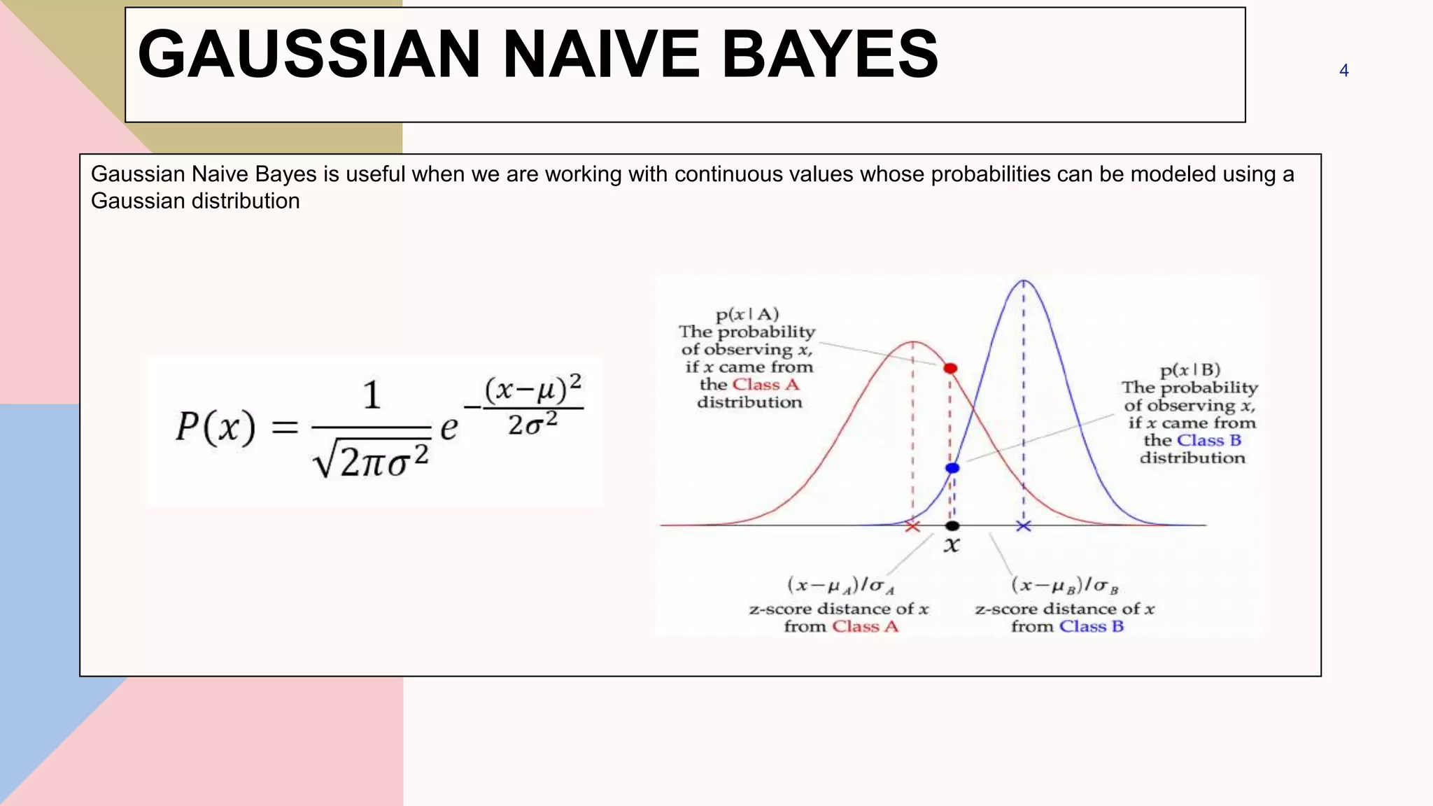
GAUSSIAN NAIVE BAYES
Gaussian Naive Bayes is useful when we are working with continuous values whose probabilities can be modeled using a
Gaussian distribution
4
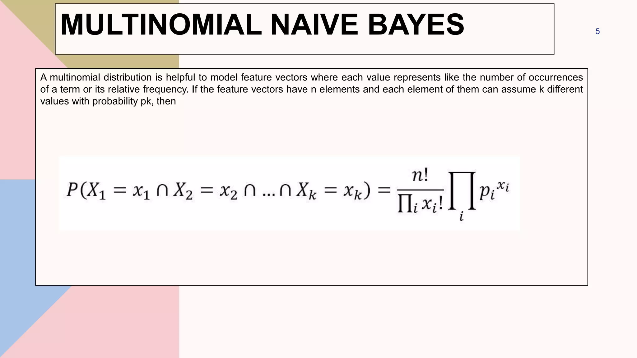
MULTINOMIAL NAIVE BAYES
A multinomial distribution is helpful to model feature vectors where each value represents like the number of occurrences
of a term or its relative frequency. If the feature vectors have n elements and each element of them can assume k different
values with probability pk, then
5
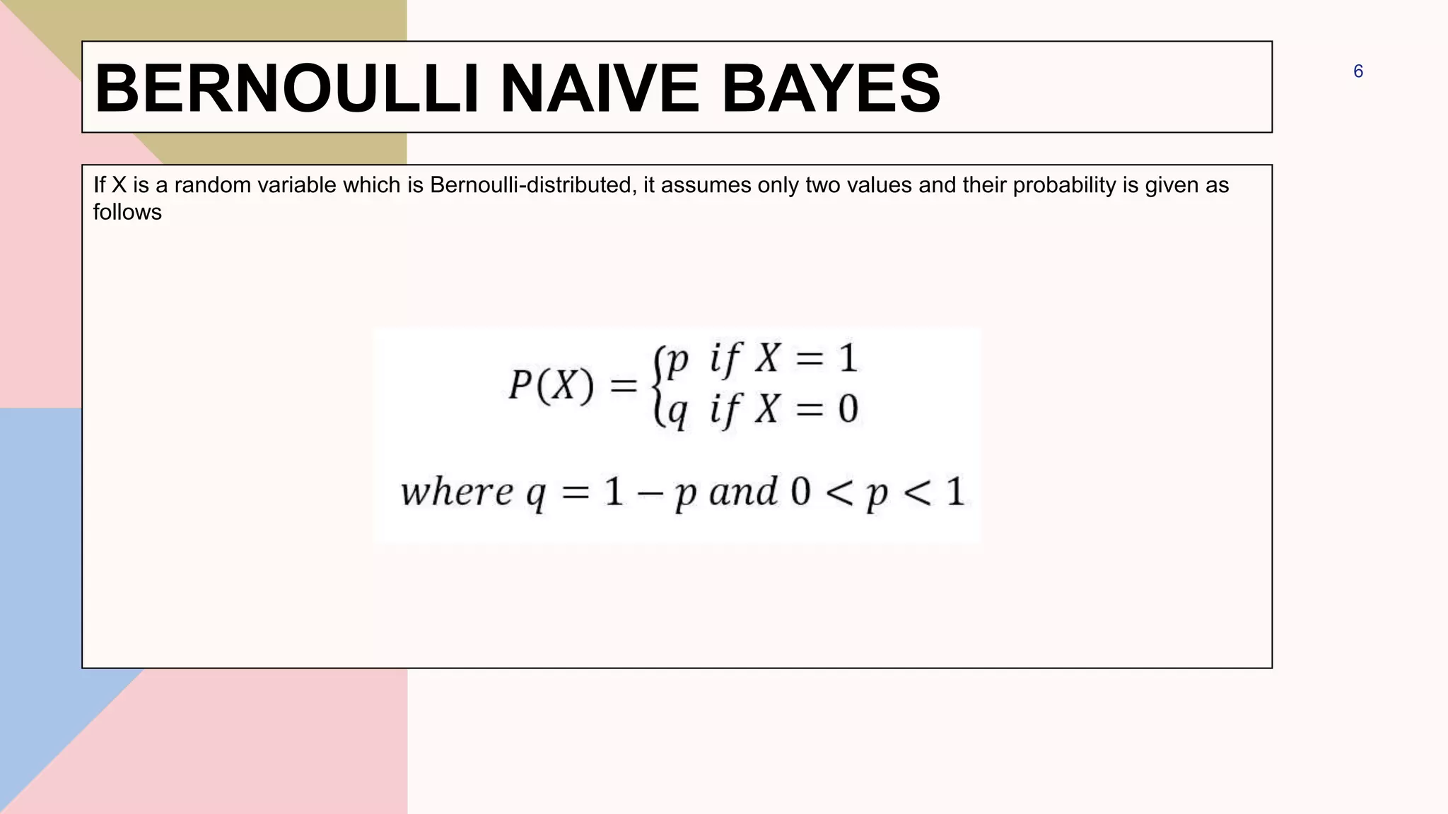
BERNOULLI NAIVE BAYES
If X is a random variable which is Bernoulli-distributed, it assumes only two values and their probability is given as
follows
6
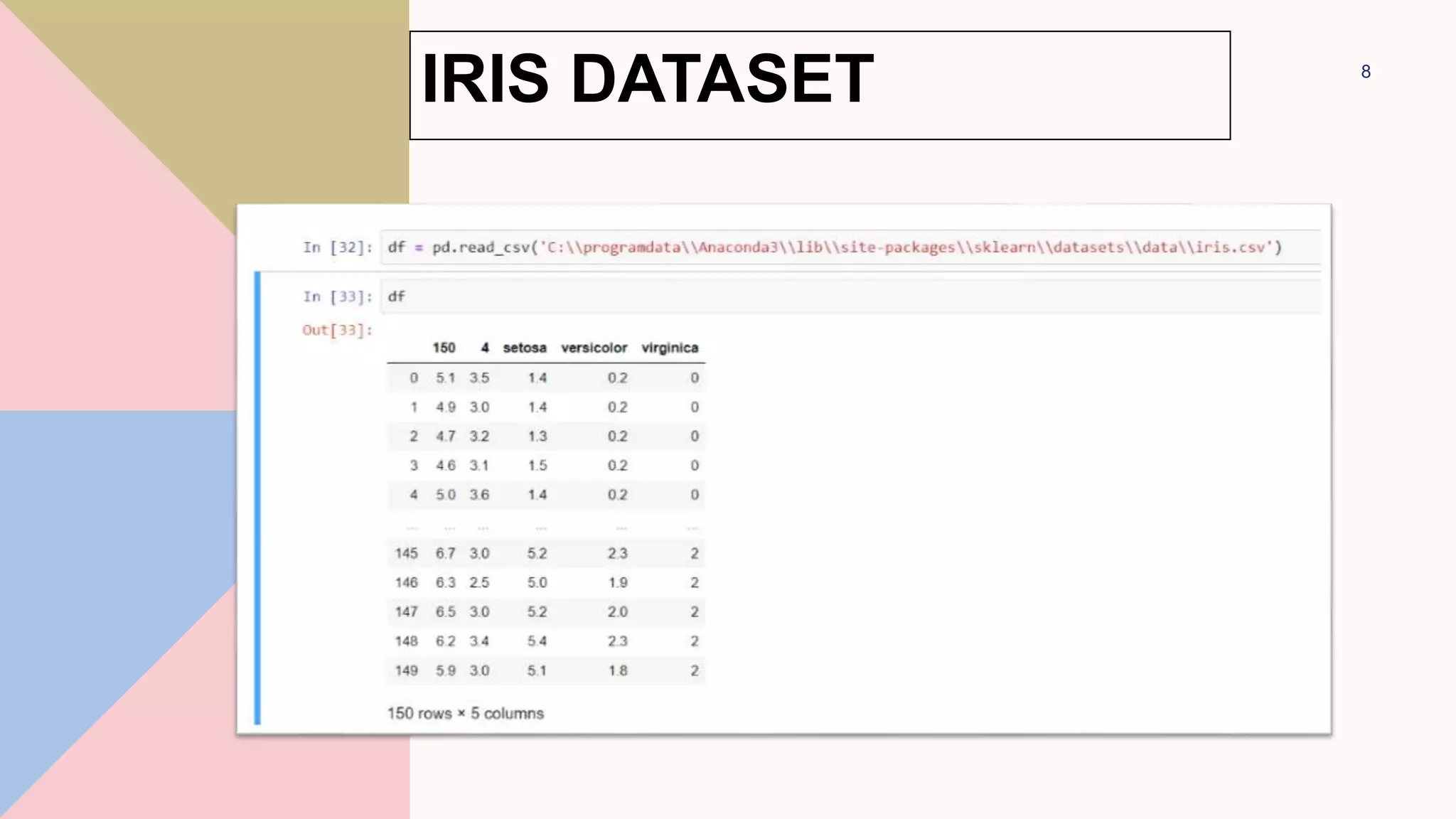
IRIS DATASET
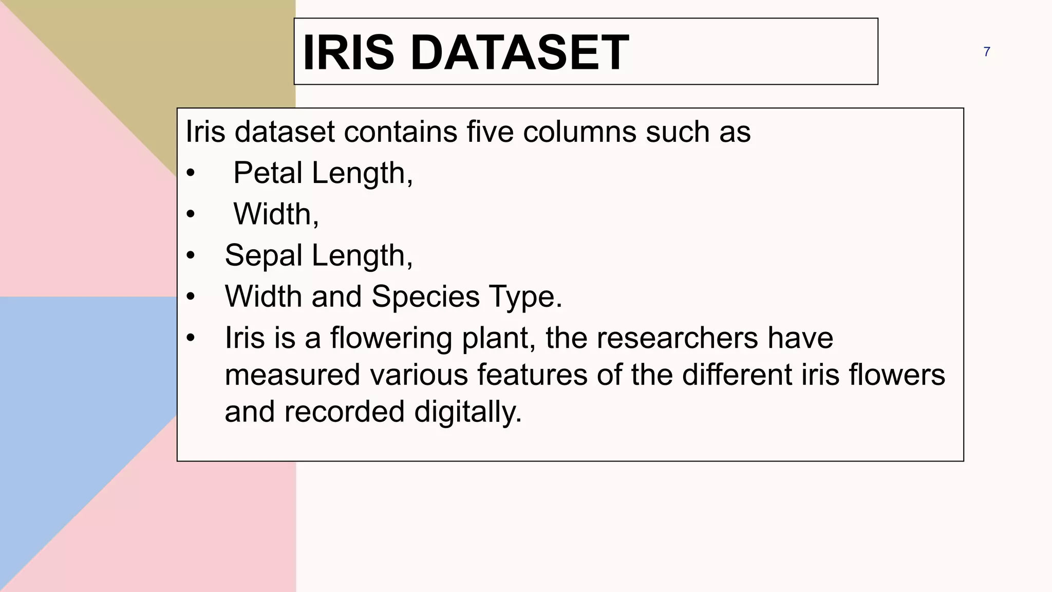
Iris dataset contains five columns such as
• Petal Length,
• Width,
• Sepal Length,
• Width and Species Type.
• Iris is a flowering plant, the researchers have
measured various features of the different iris flowers
and recorded digitally.
7
8
IRIS DATASET
9
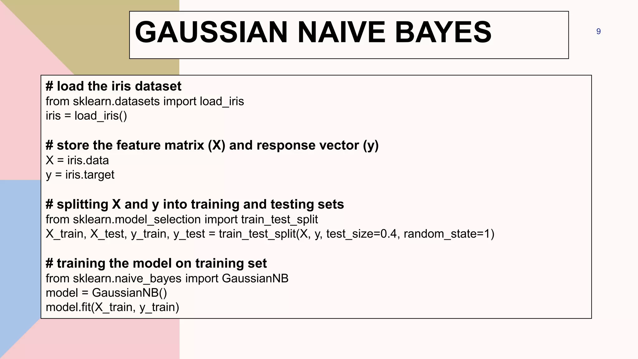
# load the iris dataset
from sklearn.datasets import load_iris
iris = load_iris()
# store the feature matrix (X) and response vector (y)
X = iris.data
y = iris.target
# splitting X and y into training and testing sets
from sklearn.model_selection import train_test_split
X_train, X_test, y_train, y_test = train_test_split(X, y, test_size=0.4, random_state=1)
# training the model on training set
from sklearn.naive_bayes import GaussianNB
model = GaussianNB()
model.fit(X_train, y_train)
GAUSSIAN NAIVE BAYES
# making predictions on the testing set
y_pred = model.predict(X_test)
# comparing actual response values (y_test) with predicted response
values (y_pred)
from sklearn.metrics import accuracy_score
print(f'Gaussian Naive Bayes model accuracy(in %):={accuracy_score(y_test,
y_pred)*100} %')
res = model.predict([[6.5,3.0,5.2,2.0]])
print(f'Result = {iris.target_names[res[0]]}')
10
GAUSSIAN NAIVE BAYES
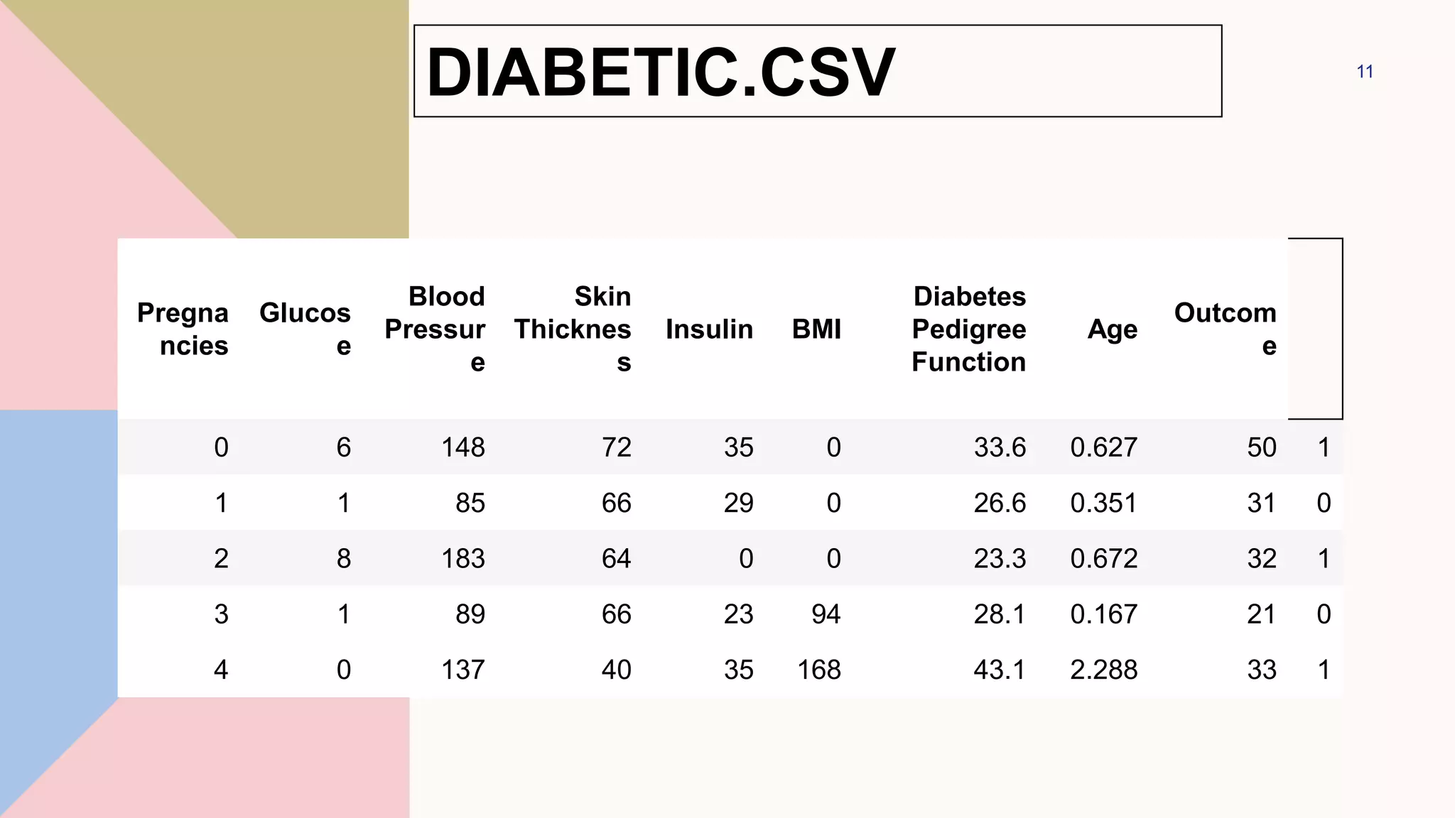
DIABETIC.CSV
Pregna
ncies
Glucos
e
Blood
Pressur
e
Skin
Thicknes
s
Insulin BMI
Diabetes
Pedigree
Function
Age
Outcom
e
0 6 148 72 35 0 33.6 0.627 50 1
1 1 85 66 29 0 26.6 0.351 31 0
2 8 183 64 0 0 23.3 0.672 32 1
3 1 89 66 23 94 28.1 0.167 21 0
4 0 137 40 35 168 43.1 2.288 33 1
11
diabetes = pd.read_csv("diabetes.csv")
diabetes.columns
Output-
12
Index(['Pregnancies', 'Glucose', 'BloodPressure',
'SkinThickness', 'Insulin', 'BMI',
'DiabetesPedigreeFunction', 'Age', 'Outcome'],
dtype='object')
DIABETIC.CSV
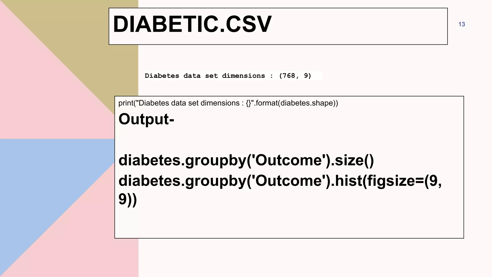
print("Diabetes data set dimensions : {}".format(diabetes.shape))
Output-
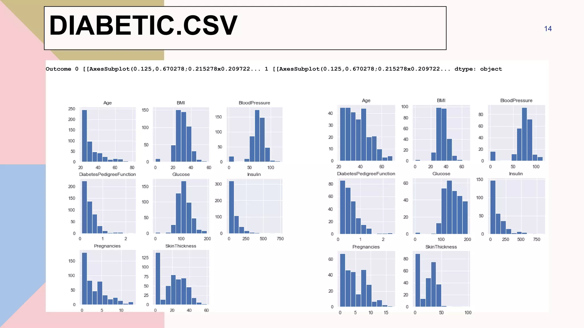
diabetes.groupby('Outcome').size()
diabetes.groupby('Outcome').hist(figsize=(9,
9))
13
Diabetes data set dimensions : (768, 9)
DIABETIC.CSV
14
Outcome 0 [[AxesSubplot(0.125,0.670278;0.215278x0.209722... 1 [[AxesSubplot(0.125,0.670278;0.215278x0.209722... dtype: object
DIABETIC.CSV
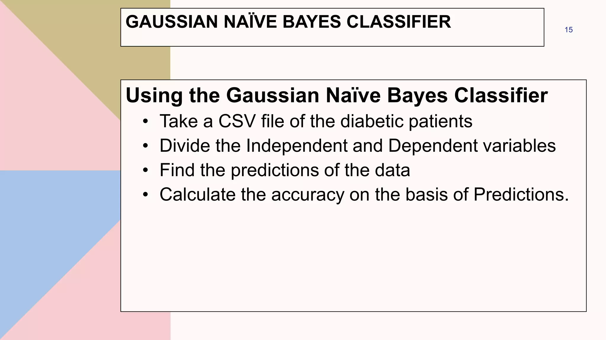
GAUSSIAN NAÏVE BAYES CLASSIFIER
Using the Gaussian Naïve Bayes Classifier
• Take a CSV file of the diabetic patients
• Divide the Independent and Dependent variables
• Find the predictions of the data
• Calculate the accuracy on the basis of Predictions.
15
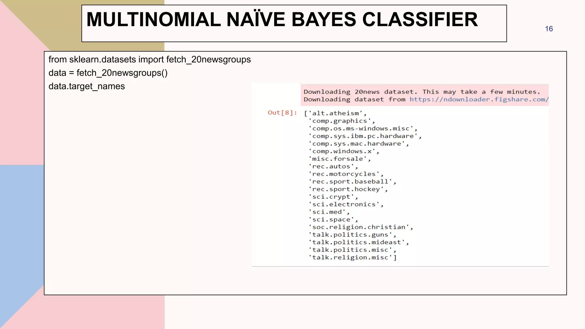
MULTINOMIAL NAÏVE BAYES CLASSIFIER
from sklearn.datasets import fetch_20newsgroups
data = fetch_20newsgroups()
data.target_names
16
categories = ['talk.religion.misc', 'soc.religion.christian’,
'sci.space', 'comp.graphics']
train = fetch_20newsgroups(subset='train', categories=categories)
test = fetch_20newsgroups(subset='test', categories=categories)
17
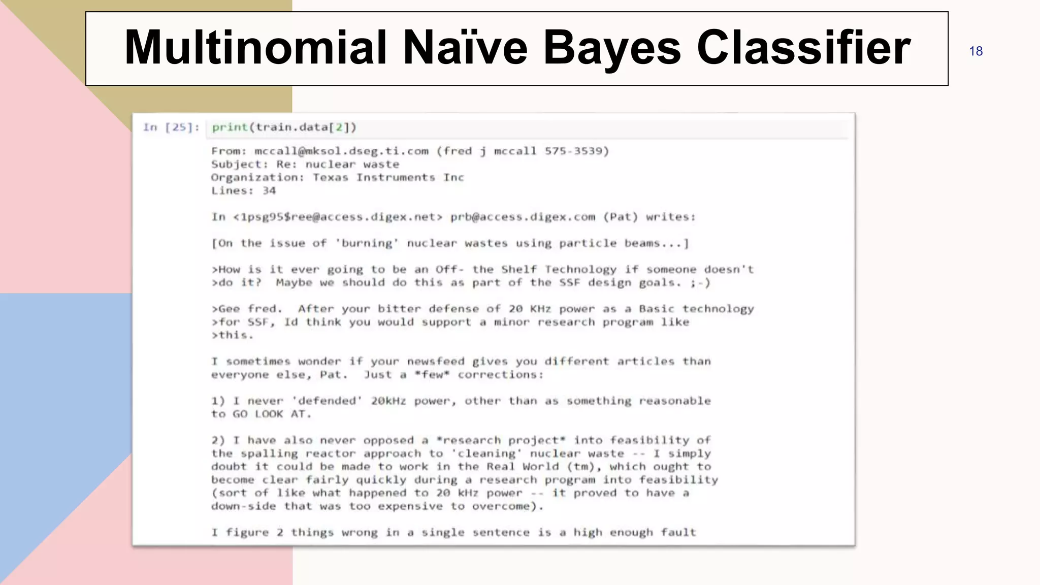
Multinomial Naïve Bayes Classifier
18
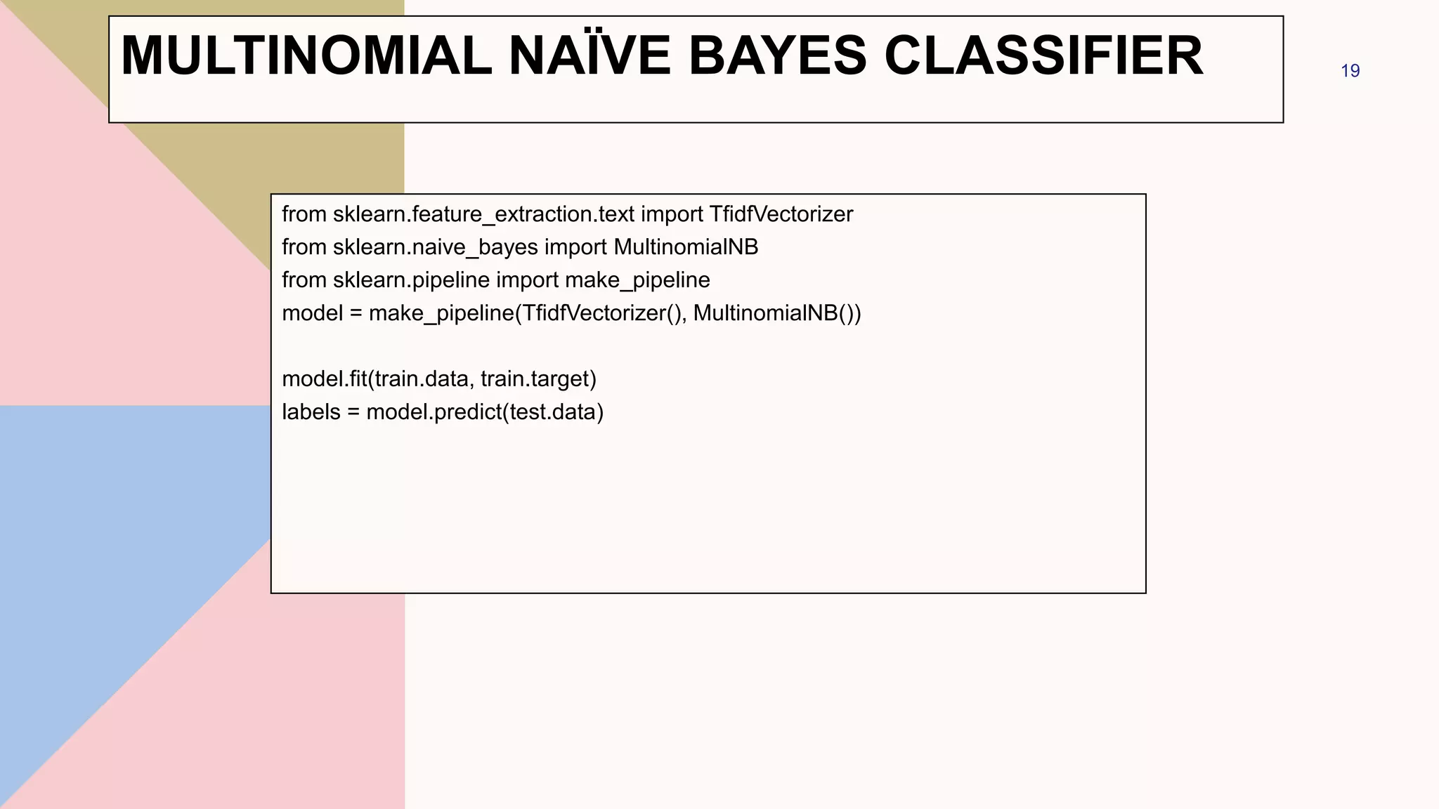
Multinomial Naïve Bayes Classifier
from sklearn.feature_extraction.text import TfidfVectorizer
from sklearn.naive_bayes import MultinomialNB
from sklearn.pipeline import make_pipeline
model = make_pipeline(TfidfVectorizer(), MultinomialNB())
model.fit(train.data, train.target)
labels = model.predict(test.data)
19
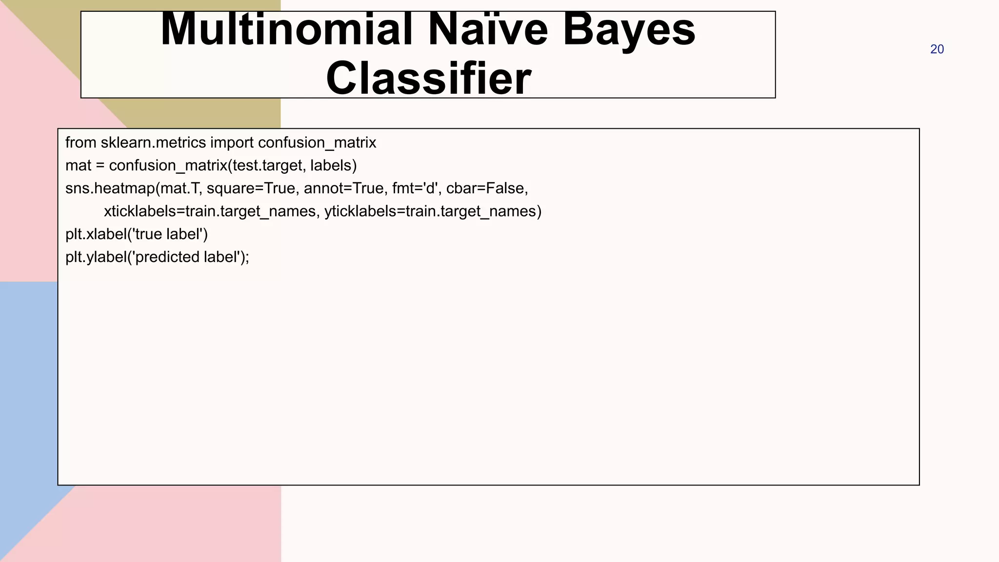
MULTINOMIAL NAÏVE BAYES CLASSIFIER
from sklearn.metrics import confusion_matrix
mat = confusion_matrix(test.target, labels)
sns.heatmap(mat.T, square=True, annot=True, fmt='d', cbar=False,
xticklabels=train.target_names, yticklabels=train.target_names)
plt.xlabel('true label')
plt.ylabel('predicted label');
20
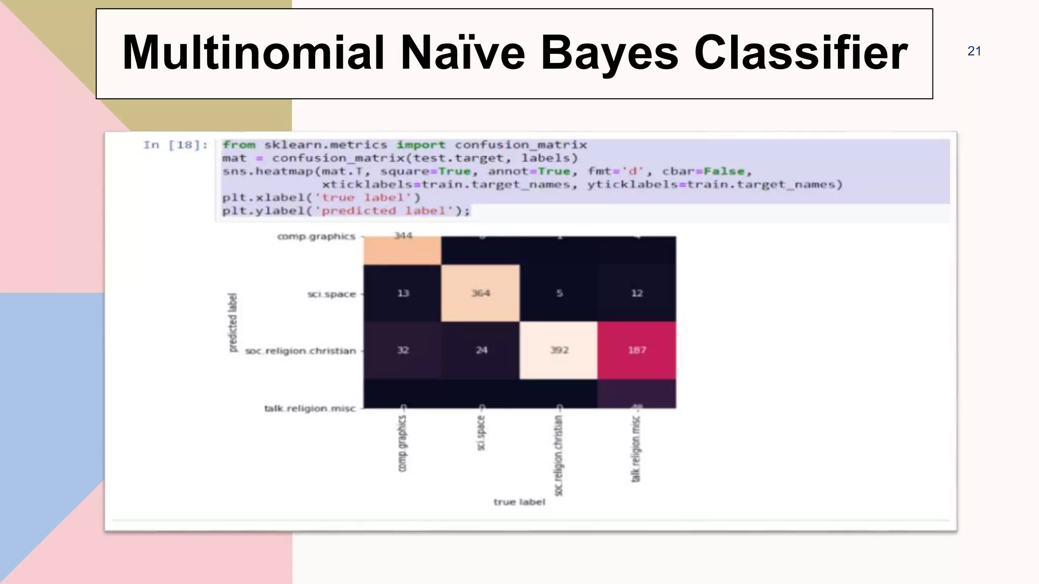
Multinomial Naïve Bayes
Classifier
21
Multinomial Naïve Bayes Classifier
def predict_category(s, train=train, model=model):
pred = model.predict([s])
return train.target_names[pred[0]]
predict_category('sending a payload to the ISS’)
Output-
22
'sci.space'
Multinomial Naïve Bayes Classifier
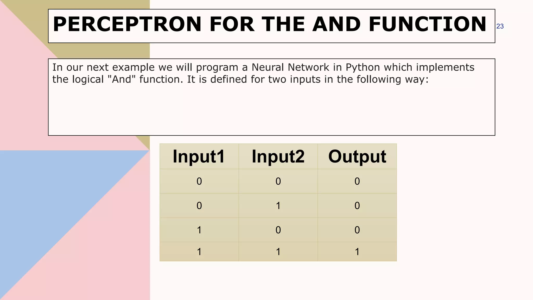
PERCEPTRON FOR THE AND FUNCTION
Input1 Input2 Output
0 0 0
0 1 0
1 0 0
1 1 1
23
In our next example we will program a Neural Network in Python which implements
the logical "And" function. It is defined for two inputs in the following way:
import matplotlib.pyplot as plt
import numpy as np
fig, ax = plt.subplots()
xmin, xmax = -0.2, 1.4
X = np.arange(xmin, xmax, 0.1)
ax.scatter(0, 0, color="r")
ax.scatter(0, 1, color="r")
ax.scatter(1, 0, color="r")
ax.scatter(1, 1, color="g")
ax.set_xlim([xmin, xmax])
ax.set_ylim([-0.1, 1.1])
m = -1
#ax.plot(X, m * X + 1.2, label="decision boundary")
plt.plot()
24
PERCEPTRON FOR THE AND FUNCTION
fig, ax = plt.subplots()
xmin, xmax = -0.2, 1.4
X = np.arange(xmin, xmax, 0.1)
ax.set_xlim([xmin, xmax])
ax.set_ylim([-0.1, 1.1])
m = -1
for m in np.arange(0, 6, 0.1):
ax.plot(X, m * X )
ax.scatter(0, 0, color="r")
ax.scatter(0, 1, color="r")
ax.scatter(1, 0, color="r")
ax.scatter(1, 1, color="g")
plt.plot()
25
PERCEPTRON FOR THE AND FUNCTION
fig, ax = plt.subplots()
xmin, xmax = -0.2, 1.4
X = np.arange(xmin, xmax, 0.1)
ax.scatter(0, 0, color="r")
ax.scatter(0, 1, color="r")
ax.scatter(1, 0, color="r")
ax.scatter(1, 1, color="g")
ax.set_xlim([xmin, xmax])
ax.set_ylim([-0.1, 1.1])
m, c = -1, 1.2
ax.plot(X, m * X + c )
plt.plot()
26
PERCEPTRON FOR THE AND FUNCTION
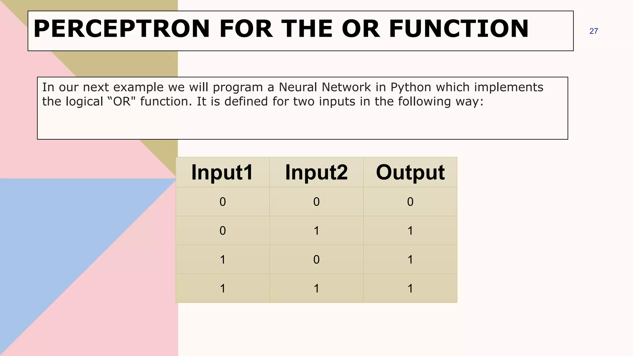
PERCEPTRON FOR THE OR FUNCTION
Input1 Input2 Output
0 0 0
0 1 1
1 0 1
1 1 1
27
In our next example we will program a Neural Network in Python which implements
the logical “OR" function. It is defined for two inputs in the following way:
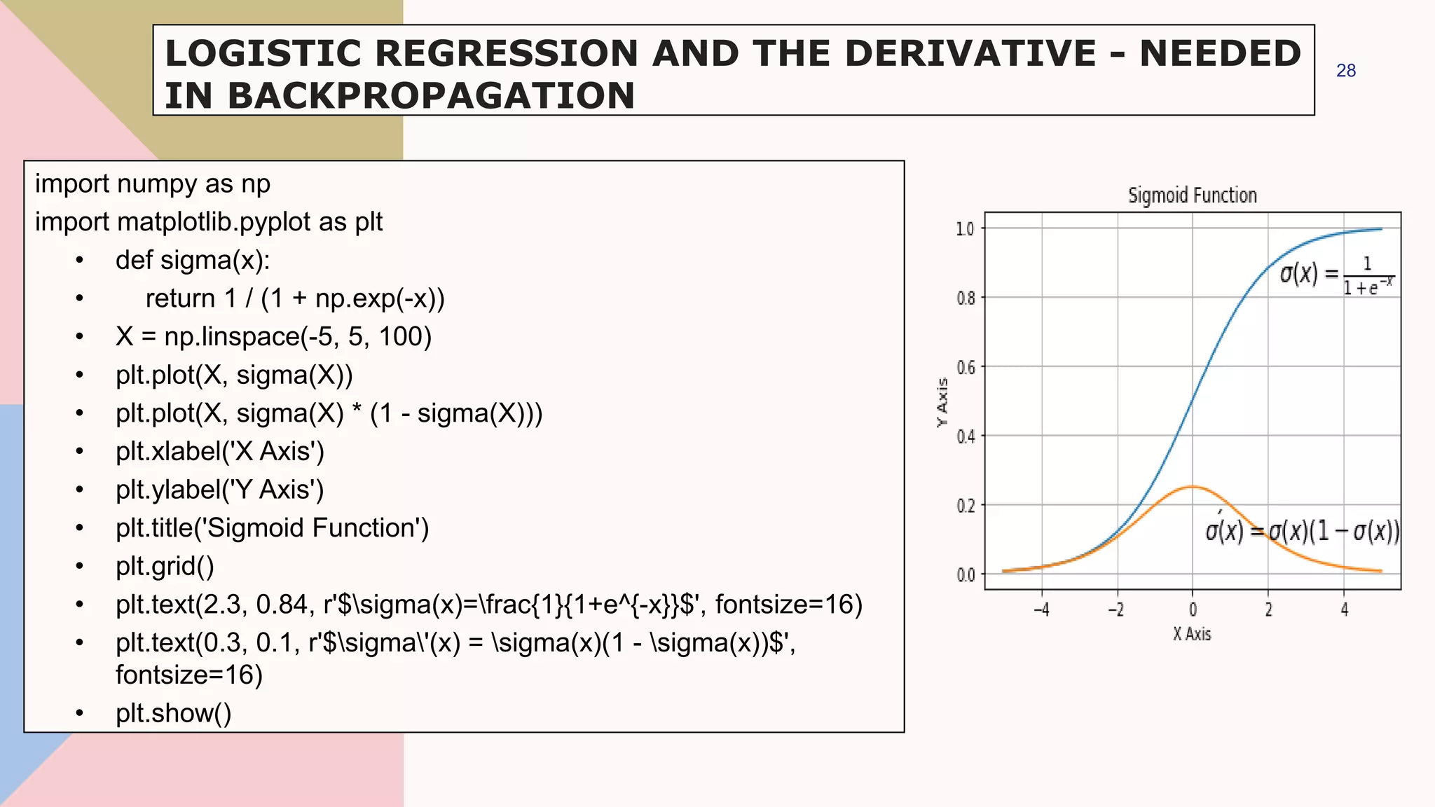
LOGISTIC REGRESSION AND THE DERIVATIVE - NEEDED
IN BACKPROPAGATION
import numpy as np
import matplotlib.pyplot as plt
• def sigma(x):
• return 1 / (1 + np.exp(-x))
• X = np.linspace(-5, 5, 100)
• plt.plot(X, sigma(X))
• plt.plot(X, sigma(X) * (1 - sigma(X)))
• plt.xlabel('X Axis')
• plt.ylabel('Y Axis')
• plt.title('Sigmoid Function')
• plt.grid()
• plt.text(2.3, 0.84, r'$sigma(x)=frac{1}{1+e^{-x}}$', fontsize=16)
• plt.text(0.3, 0.1, r'$sigma'(x) = sigma(x)(1 - sigma(x))$',
fontsize=16)
• plt.show()
28
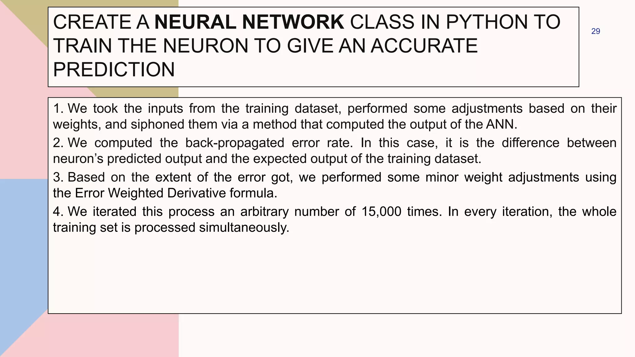
1. We took the inputs from the training dataset, performed some adjustments based on their
weights, and siphoned them via a method that computed the output of the ANN.
2. We computed the back-propagated error rate. In this case, it is the difference between
neuron’s predicted output and the expected output of the training dataset.
3. Based on the extent of the error got, we performed some minor weight adjustments using
the Error Weighted Derivative formula.
4. We iterated this process an arbitrary number of 15,000 times. In every iteration, the whole
training set is processed simultaneously.
29
CREATE A NEURAL NETWORK CLASS IN PYTHON TO
TRAIN THE NEURON TO GIVE AN ACCURATE
PREDICTION
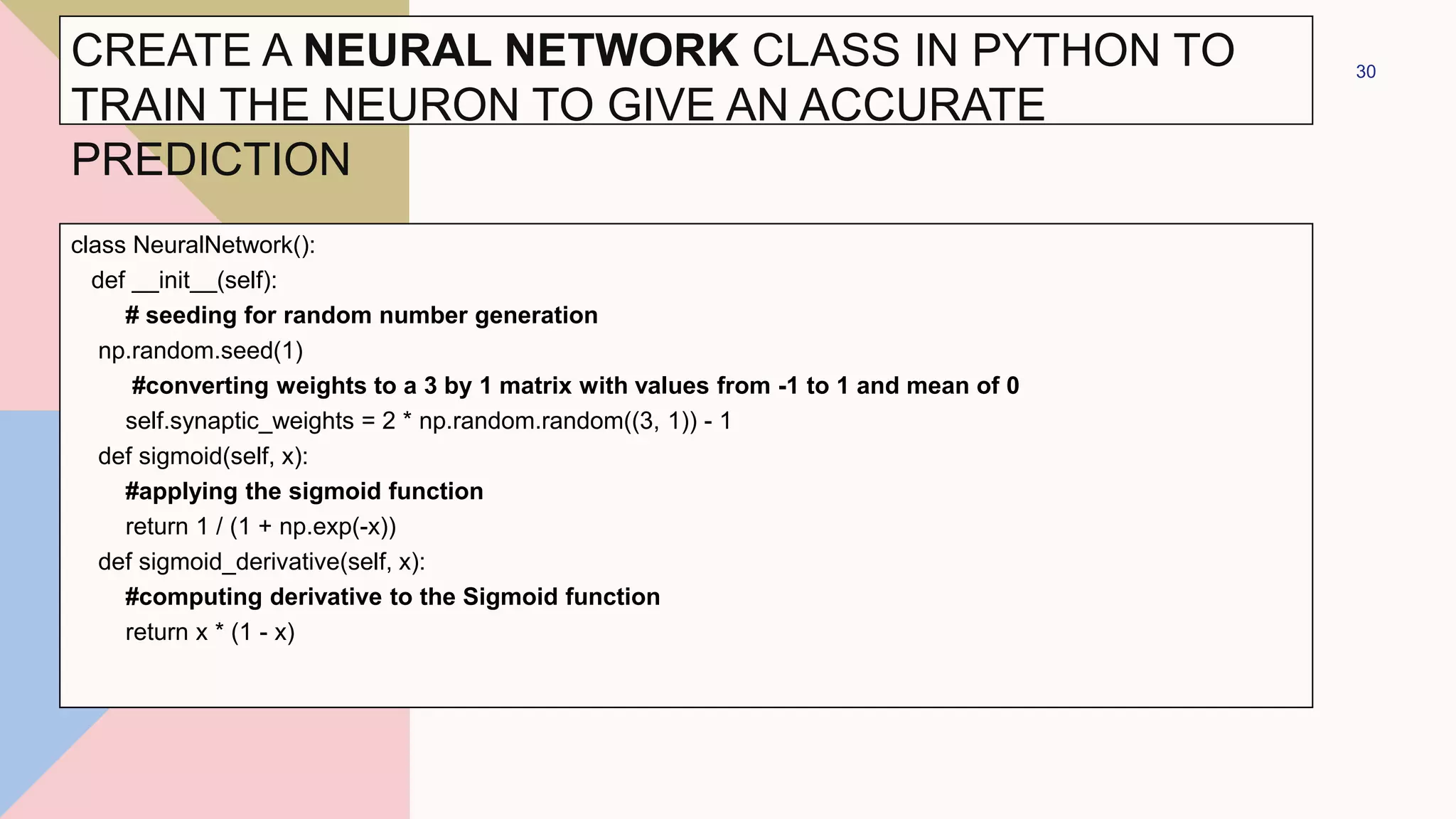
class NeuralNetwork():
def __init__(self):
# seeding for random number generation
np.random.seed(1)
#converting weights to a 3 by 1 matrix with values from -1 to 1 and mean of 0
self.synaptic_weights = 2 * np.random.random((3, 1)) - 1
def sigmoid(self, x):
#applying the sigmoid function
return 1 / (1 + np.exp(-x))
def sigmoid_derivative(self, x):
#computing derivative to the Sigmoid function
return x * (1 - x)
30
CREATE A NEURAL NETWORK CLASS IN PYTHON TO
TRAIN THE NEURON TO GIVE AN ACCURATE
PREDICTION
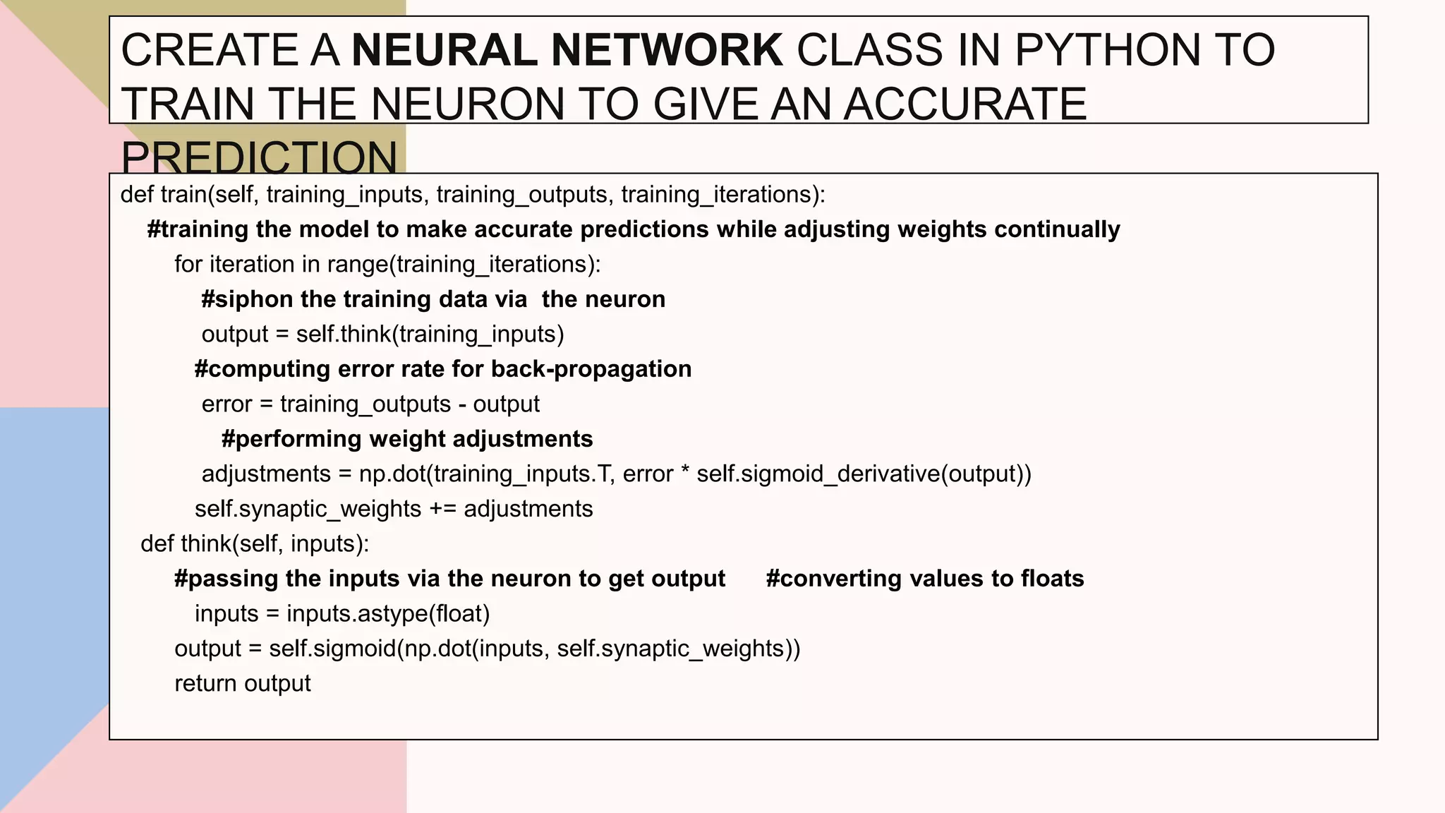
def train(self, training_inputs, training_outputs, training_iterations):
#training the model to make accurate predictions while adjusting weights continually
for iteration in range(training_iterations):
#siphon the training data via the neuron
output = self.think(training_inputs)
#computing error rate for back-propagation
error = training_outputs - output
#performing weight adjustments
adjustments = np.dot(training_inputs.T, error * self.sigmoid_derivative(output))
self.synaptic_weights += adjustments
def think(self, inputs):
#passing the inputs via the neuron to get output #converting values to floats
inputs = inputs.astype(float)
output = self.sigmoid(np.dot(inputs, self.synaptic_weights))
return output
31
CREATE A NEURAL NETWORK CLASS IN PYTHON TO
TRAIN THE NEURON TO GIVE AN ACCURATE
PREDICTION
CREATE A NEURAL NETWORK CLASS IN PYTHON TO
TRAIN THE NEURON TO GIVE AN ACCURATE
PREDICTION
training_inputs = np.array([[0,0,1],
[1,1,1],
[1,0,1],
[0,1,1]])
training_outputs = np.array([[0,1,1,0]]).T
#training taking place
neural_network.train(training_inputs, training_outputs, 15000)
print("Ending Weights After Training: ")
print(neural_network.synaptic_weights)
32
PYTHON PROGRAMMING-ANACONDA
• Anaconda is a free and open source distribution of the Python and R
programming languages for large-scale data processing, predictive analytics, and
scientific computing.
• The advantage of Anaconda is that you have access to over 720 packages that
can easily be installed with Anaconda's Conda, a package, dependency, and
environment manager.
• Anaconda distribution is available for installation
at https://www.anaconda.com/download/. For installation on Windows, 32 and 64
bit binaries are available −
33
PYTHON PROGRAMMING
Online Compiler:-
https://dataplatform.cloud.ibm.com/
https://jupyter.org/
https://colab.research.google.com/
34
THANK YOU
aman_preet_k@yahoo.co.in

Naïve Bayes.pptx

  • 1.
    NAÏVE BAYES Dr. AmanpreetKaur​ Associate Professor, Chitkara University, Punjab
  • 2.
    AGENDA - TYPESOF NAÏVE BAYES CLASSIFIERS There are three types of classifiers. They are • Gaussian Naïve Bayes • Multinomial Naïve Bayes • Bernoulli Naïve Bayes
  • 3.
    • When workingwith continuous data, an assumption often taken is that the continuous values associated with each class are distributed according to a normal (or Gaussian) distribution. • For example, suppose the training data contains a continuous attribute , X • We first segment the data by the class, and then compute the mean and Variance of X in each class. 3 GAUSSIAN NAIVE BAYES
  • 4.
    GAUSSIAN NAIVE BAYES GaussianNaive Bayes is useful when we are working with continuous values whose probabilities can be modeled using a Gaussian distribution 4
  • 5.
    MULTINOMIAL NAIVE BAYES Amultinomial distribution is helpful to model feature vectors where each value represents like the number of occurrences of a term or its relative frequency. If the feature vectors have n elements and each element of them can assume k different values with probability pk, then 5
  • 6.
    BERNOULLI NAIVE BAYES IfX is a random variable which is Bernoulli-distributed, it assumes only two values and their probability is given as follows 6
  • 7.
    IRIS DATASET Iris datasetcontains five columns such as • Petal Length, • Width, • Sepal Length, • Width and Species Type. • Iris is a flowering plant, the researchers have measured various features of the different iris flowers and recorded digitally. 7
  • 8.
  • 9.
    9 # load theiris dataset from sklearn.datasets import load_iris iris = load_iris() # store the feature matrix (X) and response vector (y) X = iris.data y = iris.target # splitting X and y into training and testing sets from sklearn.model_selection import train_test_split X_train, X_test, y_train, y_test = train_test_split(X, y, test_size=0.4, random_state=1) # training the model on training set from sklearn.naive_bayes import GaussianNB model = GaussianNB() model.fit(X_train, y_train) GAUSSIAN NAIVE BAYES
  • 10.
    # making predictionson the testing set y_pred = model.predict(X_test) # comparing actual response values (y_test) with predicted response values (y_pred) from sklearn.metrics import accuracy_score print(f'Gaussian Naive Bayes model accuracy(in %):={accuracy_score(y_test, y_pred)*100} %') res = model.predict([[6.5,3.0,5.2,2.0]]) print(f'Result = {iris.target_names[res[0]]}') 10 GAUSSIAN NAIVE BAYES
  • 11.
    DIABETIC.CSV Pregna ncies Glucos e Blood Pressur e Skin Thicknes s Insulin BMI Diabetes Pedigree Function Age Outcom e 0 6148 72 35 0 33.6 0.627 50 1 1 1 85 66 29 0 26.6 0.351 31 0 2 8 183 64 0 0 23.3 0.672 32 1 3 1 89 66 23 94 28.1 0.167 21 0 4 0 137 40 35 168 43.1 2.288 33 1 11
  • 12.
    diabetes = pd.read_csv("diabetes.csv") diabetes.columns Output- 12 Index(['Pregnancies','Glucose', 'BloodPressure', 'SkinThickness', 'Insulin', 'BMI', 'DiabetesPedigreeFunction', 'Age', 'Outcome'], dtype='object') DIABETIC.CSV
  • 13.
    print("Diabetes data setdimensions : {}".format(diabetes.shape)) Output- diabetes.groupby('Outcome').size() diabetes.groupby('Outcome').hist(figsize=(9, 9)) 13 Diabetes data set dimensions : (768, 9) DIABETIC.CSV
  • 14.
    14 Outcome 0 [[AxesSubplot(0.125,0.670278;0.215278x0.209722...1 [[AxesSubplot(0.125,0.670278;0.215278x0.209722... dtype: object DIABETIC.CSV
  • 15.
    GAUSSIAN NAÏVE BAYESCLASSIFIER Using the Gaussian Naïve Bayes Classifier • Take a CSV file of the diabetic patients • Divide the Independent and Dependent variables • Find the predictions of the data • Calculate the accuracy on the basis of Predictions. 15
  • 16.
    MULTINOMIAL NAÏVE BAYESCLASSIFIER from sklearn.datasets import fetch_20newsgroups data = fetch_20newsgroups() data.target_names 16
  • 17.
    categories = ['talk.religion.misc','soc.religion.christian’, 'sci.space', 'comp.graphics'] train = fetch_20newsgroups(subset='train', categories=categories) test = fetch_20newsgroups(subset='test', categories=categories) 17 Multinomial Naïve Bayes Classifier
  • 18.
  • 19.
    from sklearn.feature_extraction.text importTfidfVectorizer from sklearn.naive_bayes import MultinomialNB from sklearn.pipeline import make_pipeline model = make_pipeline(TfidfVectorizer(), MultinomialNB()) model.fit(train.data, train.target) labels = model.predict(test.data) 19 MULTINOMIAL NAÏVE BAYES CLASSIFIER
  • 20.
    from sklearn.metrics importconfusion_matrix mat = confusion_matrix(test.target, labels) sns.heatmap(mat.T, square=True, annot=True, fmt='d', cbar=False, xticklabels=train.target_names, yticklabels=train.target_names) plt.xlabel('true label') plt.ylabel('predicted label'); 20 Multinomial Naïve Bayes Classifier
  • 21.
  • 22.
    def predict_category(s, train=train,model=model): pred = model.predict([s]) return train.target_names[pred[0]] predict_category('sending a payload to the ISS’) Output- 22 'sci.space' Multinomial Naïve Bayes Classifier
  • 23.
    PERCEPTRON FOR THEAND FUNCTION Input1 Input2 Output 0 0 0 0 1 0 1 0 0 1 1 1 23 In our next example we will program a Neural Network in Python which implements the logical "And" function. It is defined for two inputs in the following way:
  • 24.
    import matplotlib.pyplot asplt import numpy as np fig, ax = plt.subplots() xmin, xmax = -0.2, 1.4 X = np.arange(xmin, xmax, 0.1) ax.scatter(0, 0, color="r") ax.scatter(0, 1, color="r") ax.scatter(1, 0, color="r") ax.scatter(1, 1, color="g") ax.set_xlim([xmin, xmax]) ax.set_ylim([-0.1, 1.1]) m = -1 #ax.plot(X, m * X + 1.2, label="decision boundary") plt.plot() 24 PERCEPTRON FOR THE AND FUNCTION
  • 25.
    fig, ax =plt.subplots() xmin, xmax = -0.2, 1.4 X = np.arange(xmin, xmax, 0.1) ax.set_xlim([xmin, xmax]) ax.set_ylim([-0.1, 1.1]) m = -1 for m in np.arange(0, 6, 0.1): ax.plot(X, m * X ) ax.scatter(0, 0, color="r") ax.scatter(0, 1, color="r") ax.scatter(1, 0, color="r") ax.scatter(1, 1, color="g") plt.plot() 25 PERCEPTRON FOR THE AND FUNCTION
  • 26.
    fig, ax =plt.subplots() xmin, xmax = -0.2, 1.4 X = np.arange(xmin, xmax, 0.1) ax.scatter(0, 0, color="r") ax.scatter(0, 1, color="r") ax.scatter(1, 0, color="r") ax.scatter(1, 1, color="g") ax.set_xlim([xmin, xmax]) ax.set_ylim([-0.1, 1.1]) m, c = -1, 1.2 ax.plot(X, m * X + c ) plt.plot() 26 PERCEPTRON FOR THE AND FUNCTION
  • 27.
    PERCEPTRON FOR THEOR FUNCTION Input1 Input2 Output 0 0 0 0 1 1 1 0 1 1 1 1 27 In our next example we will program a Neural Network in Python which implements the logical “OR" function. It is defined for two inputs in the following way:
  • 28.
    LOGISTIC REGRESSION ANDTHE DERIVATIVE - NEEDED IN BACKPROPAGATION import numpy as np import matplotlib.pyplot as plt • def sigma(x): • return 1 / (1 + np.exp(-x)) • X = np.linspace(-5, 5, 100) • plt.plot(X, sigma(X)) • plt.plot(X, sigma(X) * (1 - sigma(X))) • plt.xlabel('X Axis') • plt.ylabel('Y Axis') • plt.title('Sigmoid Function') • plt.grid() • plt.text(2.3, 0.84, r'$sigma(x)=frac{1}{1+e^{-x}}$', fontsize=16) • plt.text(0.3, 0.1, r'$sigma'(x) = sigma(x)(1 - sigma(x))$', fontsize=16) • plt.show() 28
  • 29.
    1. We tookthe inputs from the training dataset, performed some adjustments based on their weights, and siphoned them via a method that computed the output of the ANN. 2. We computed the back-propagated error rate. In this case, it is the difference between neuron’s predicted output and the expected output of the training dataset. 3. Based on the extent of the error got, we performed some minor weight adjustments using the Error Weighted Derivative formula. 4. We iterated this process an arbitrary number of 15,000 times. In every iteration, the whole training set is processed simultaneously. 29 CREATE A NEURAL NETWORK CLASS IN PYTHON TO TRAIN THE NEURON TO GIVE AN ACCURATE PREDICTION
  • 30.
    class NeuralNetwork(): def __init__(self): #seeding for random number generation np.random.seed(1) #converting weights to a 3 by 1 matrix with values from -1 to 1 and mean of 0 self.synaptic_weights = 2 * np.random.random((3, 1)) - 1 def sigmoid(self, x): #applying the sigmoid function return 1 / (1 + np.exp(-x)) def sigmoid_derivative(self, x): #computing derivative to the Sigmoid function return x * (1 - x) 30 CREATE A NEURAL NETWORK CLASS IN PYTHON TO TRAIN THE NEURON TO GIVE AN ACCURATE PREDICTION
  • 31.
    def train(self, training_inputs,training_outputs, training_iterations): #training the model to make accurate predictions while adjusting weights continually for iteration in range(training_iterations): #siphon the training data via the neuron output = self.think(training_inputs) #computing error rate for back-propagation error = training_outputs - output #performing weight adjustments adjustments = np.dot(training_inputs.T, error * self.sigmoid_derivative(output)) self.synaptic_weights += adjustments def think(self, inputs): #passing the inputs via the neuron to get output #converting values to floats inputs = inputs.astype(float) output = self.sigmoid(np.dot(inputs, self.synaptic_weights)) return output 31 CREATE A NEURAL NETWORK CLASS IN PYTHON TO TRAIN THE NEURON TO GIVE AN ACCURATE PREDICTION
  • 32.
    CREATE A NEURALNETWORK CLASS IN PYTHON TO TRAIN THE NEURON TO GIVE AN ACCURATE PREDICTION training_inputs = np.array([[0,0,1], [1,1,1], [1,0,1], [0,1,1]]) training_outputs = np.array([[0,1,1,0]]).T #training taking place neural_network.train(training_inputs, training_outputs, 15000) print("Ending Weights After Training: ") print(neural_network.synaptic_weights) 32
  • 33.
    PYTHON PROGRAMMING-ANACONDA • Anacondais a free and open source distribution of the Python and R programming languages for large-scale data processing, predictive analytics, and scientific computing. • The advantage of Anaconda is that you have access to over 720 packages that can easily be installed with Anaconda's Conda, a package, dependency, and environment manager. • Anaconda distribution is available for installation at https://www.anaconda.com/download/. For installation on Windows, 32 and 64 bit binaries are available − 33
  • 34.
  • 35.