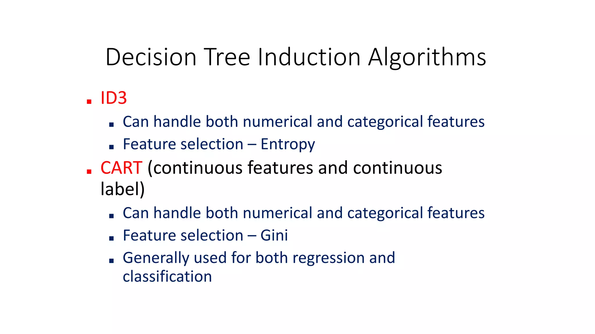
BCSE209L Machine Learning
Module- : Decision Trees
Dr. R. Jothi
Decision Tree Induction Algorithms
■ ID3
■ Can handle both numerical and categorical features
■ Feature selection – Entropy
■ CART (continuous features and continuous
label)
■ Can handle both numerical and categorical features
■ Feature selection – Gini
■ Generally used for both regression and
classification
Measure of Impurity: GINI
• The Gini Index is the probability that a variable will not
be classified correctly if it was chosen randomly.
• Gini Index for a given node t with classes j
NOTE: p( j | t) is computed as the relative frequency of class j at
node t



j
t
j
p
t
GINI 2
)]
|
(
[
1
)
(
3
GINI Index : Example
• Example: Two classes C1 & C2 and node t has 5 C1 and
5 C2 examples. Compute Gini(t)
• 1 – [p(C1|t) + p(C2|t)] = 1 – [(5/10)2 + [(5/10)2 ]
• 1 – [¼ + ¼] = ½.



j
t
j
p
t
GINI 2
)]
|
(
[
1
)
(
4
The Gini index will always be between [0, 0.5], where 0 is
a selection that perfectly splits each class in your dataset
(pure), and 0.5 means that neither of the classes was
correctly classified (impure).
More on Gini
• Worst Gini corresponds to probabilities of 1/nc, where nc is the number of
classes.
• For 2-class problems the worst Gini will be ½
• How do we get the best Gini? Come up with an example for node t with 10
examples for classes C1 and C2
• 10 C1 and 0 C2
• Now what is the Gini?
• 1 – [(10/10)2 + (0/10)2 = 1 – [1 + 0] = 0
• So 0 is the best Gini
• So for 2-class problems:
• Gini varies from 0 (best) to ½ (worst).
5
Some More Examples
• Below we see the Gini values for 4 nodes with
different distributions. They are ordered from best to
worst. See next slide for details
• Note that thus far we are only computing GINI for one node.
We need to compute it for a split and then compute the
change in Gini from the parent node.
C1 0
C2 6
Gini=0.000
C1 2
C2 4
Gini=0.444
C1 3
C2 3
Gini=0.500
C1 1
C2 5
Gini=0.278
6
Examples for computing GINI
C1 0
C2 6
C1 2
C2 4
C1 1
C2 5
P(C1) = 0/6 = 0 P(C2) = 6/6 = 1
Gini = 1 – P(C1)2 – P(C2)2 = 1 – 0 – 1 = 0



j
t
j
p
t
GINI 2
)]
|
(
[
1
)
(
P(C1) = 1/6 P(C2) = 5/6
Gini = 1 – (1/6)2 – (5/6)2 = 0.278
P(C1) = 2/6 P(C2) = 4/6
Gini = 1 – (2/6)2 – (4/6)2 = 0.444
Examples for Computing Error
C1 0
C2 6
C1 2
C2 4
C1 1
C2 5
P(C1) = 0/6 = 0 P(C2) = 6/6 = 1
Error = 1 – max (0, 1) = 1 – 1 = 0
P(C1) = 1/6 P(C2) = 5/6
Error = 1 – max (1/6, 5/6) = 1 – 5/6 = 1/6
P(C1) = 2/6 P(C2) = 4/6
Error = 1 – max (2/6, 4/6) = 1 – 4/6 = 1/3
)
|
(
max
1
)
( t
i
P
t
Error i


8
CSEDIU
Comparison among Splitting Criteria
For a 2-class problem:
9
CSEDIU
Example: Construct Decision tree using Gini
index
Example: Construct Decision tree using Gini
index
Therefore, attribute B will be chosen to split the node.
Gini vs Entropy
•Computationally, entropy is more complex since it makes use
of logarithms and consequently, the calculation of the Gini Index
will be faster.
• Accuracy using the entropy criterion are slightly better (not
always).
Table 11.6
Algorithm Splitting Criteria Remark
ID3 Information Gain
𝛼 𝐴, 𝐷 = 𝐸 𝐷 − 𝐸𝐴(D)
Where
𝐸 𝐷 = Entropy of D (a
measure of uncertainty) =
− 𝑖=1
𝑘
𝑝𝑖 log 2𝑝𝑖
where D is with set of k classes
𝑐1, 𝑐2, … , 𝑐𝑘 and 𝑝𝑖 =
|𝐶𝑖,𝐷|
|𝐷|
;
Here, 𝐶𝑖,𝐷 is the set of tuples
with class 𝑐𝑖 in D.
𝐸𝐴 (D) = Weighted average
entropy when D is partitioned
on the values of attribute A =
𝑗=1
𝑚 |𝐷𝑗|
|𝐷|
𝐸(𝐷𝑗)
Here, m denotes the distinct
values of attribute A.
• The algorithm calculates
𝛼(𝐴𝑖,D) for all 𝐴𝑖 in D
and choose that attribute
which has maximum
𝛼(𝐴𝑖,D).
• The algorithm can handle
both categorical and
numerical attributes.
• It favors splitting those
attributes, which has a
large number of distinct
values.
13
Algorithm Splitting Criteria Remark
CART Gini Index
𝛾 𝐴, 𝐷 = 𝐺 𝐷 − 𝐺𝐴(D)
where
𝐺 𝐷 = Gini index (a measure of
impurity)
= 1 − 𝑖=1
𝑘
𝑝𝑖
2
Here, 𝑝𝑖 =
|𝐶𝑖,𝐷|
|𝐷|
and D is with k
number of classes and
GA(D) =
|𝐷1|
|𝐷|
𝐺(𝐷1) +
|𝐷2|
|𝐷|
𝐺(𝐷2),
when D is partitioned into two
data sets 𝐷1 and 𝐷2 based on
some values of attribute A.
• The algorithm calculates
all binary partitions for
all possible values of
attribute A and choose
that binary partition
which has the maximum
𝛾 𝐴, 𝐷 .
• The algorithm is
computationally very
expensive when the
attribute A has a large
number of values.
14
Algorithm Splitting Criteria Remark
C4.5 Gain Ratio
𝛽 𝐴, 𝐷 =
𝛼 𝐴, 𝐷
𝐸𝐴
∗
(D)
where
𝛼 𝐴, 𝐷 = Information gain of
D (same as in ID3, and
𝐸𝐴
∗
(D) = splitting information
= − 𝑗=1
𝑚 |𝐷𝑗|
|𝐷|
𝑙𝑜𝑔2
|𝐷𝑗|
|𝐷|
when D is partitioned into 𝐷1,
𝐷2, … , 𝐷𝑚 partitions
corresponding to m distinct
attribute values of A.
• The attribute A with
maximum value of
𝛽 𝐴, 𝐷 is selected for
splitting.
• Splitting information is a
kind of normalization, so
that it can check the
biasness of information
gain towards the
choosing attributes with a
large number of distinct
values.
In addition to this, we also highlight few important characteristics
of decision tree induction algorithms in the following.
15

ML Decision Tree_2.pptx

  • 1.
    BCSE209L Machine Learning Module-: Decision Trees Dr. R. Jothi
  • 2.
    Decision Tree InductionAlgorithms ■ ID3 ■ Can handle both numerical and categorical features ■ Feature selection – Entropy ■ CART (continuous features and continuous label) ■ Can handle both numerical and categorical features ■ Feature selection – Gini ■ Generally used for both regression and classification
  • 3.
    Measure of Impurity:GINI • The Gini Index is the probability that a variable will not be classified correctly if it was chosen randomly. • Gini Index for a given node t with classes j NOTE: p( j | t) is computed as the relative frequency of class j at node t    j t j p t GINI 2 )] | ( [ 1 ) ( 3
  • 4.
    GINI Index :Example • Example: Two classes C1 & C2 and node t has 5 C1 and 5 C2 examples. Compute Gini(t) • 1 – [p(C1|t) + p(C2|t)] = 1 – [(5/10)2 + [(5/10)2 ] • 1 – [¼ + ¼] = ½.    j t j p t GINI 2 )] | ( [ 1 ) ( 4 The Gini index will always be between [0, 0.5], where 0 is a selection that perfectly splits each class in your dataset (pure), and 0.5 means that neither of the classes was correctly classified (impure).
  • 5.
    More on Gini •Worst Gini corresponds to probabilities of 1/nc, where nc is the number of classes. • For 2-class problems the worst Gini will be ½ • How do we get the best Gini? Come up with an example for node t with 10 examples for classes C1 and C2 • 10 C1 and 0 C2 • Now what is the Gini? • 1 – [(10/10)2 + (0/10)2 = 1 – [1 + 0] = 0 • So 0 is the best Gini • So for 2-class problems: • Gini varies from 0 (best) to ½ (worst). 5
  • 6.
    Some More Examples •Below we see the Gini values for 4 nodes with different distributions. They are ordered from best to worst. See next slide for details • Note that thus far we are only computing GINI for one node. We need to compute it for a split and then compute the change in Gini from the parent node. C1 0 C2 6 Gini=0.000 C1 2 C2 4 Gini=0.444 C1 3 C2 3 Gini=0.500 C1 1 C2 5 Gini=0.278 6
  • 7.
    Examples for computingGINI C1 0 C2 6 C1 2 C2 4 C1 1 C2 5 P(C1) = 0/6 = 0 P(C2) = 6/6 = 1 Gini = 1 – P(C1)2 – P(C2)2 = 1 – 0 – 1 = 0    j t j p t GINI 2 )] | ( [ 1 ) ( P(C1) = 1/6 P(C2) = 5/6 Gini = 1 – (1/6)2 – (5/6)2 = 0.278 P(C1) = 2/6 P(C2) = 4/6 Gini = 1 – (2/6)2 – (4/6)2 = 0.444
  • 8.
    Examples for ComputingError C1 0 C2 6 C1 2 C2 4 C1 1 C2 5 P(C1) = 0/6 = 0 P(C2) = 6/6 = 1 Error = 1 – max (0, 1) = 1 – 1 = 0 P(C1) = 1/6 P(C2) = 5/6 Error = 1 – max (1/6, 5/6) = 1 – 5/6 = 1/6 P(C1) = 2/6 P(C2) = 4/6 Error = 1 – max (2/6, 4/6) = 1 – 4/6 = 1/3 ) | ( max 1 ) ( t i P t Error i   8 CSEDIU
  • 9.
    Comparison among SplittingCriteria For a 2-class problem: 9 CSEDIU
  • 10.
    Example: Construct Decisiontree using Gini index
  • 11.
    Example: Construct Decisiontree using Gini index Therefore, attribute B will be chosen to split the node.
  • 12.
    Gini vs Entropy •Computationally,entropy is more complex since it makes use of logarithms and consequently, the calculation of the Gini Index will be faster. • Accuracy using the entropy criterion are slightly better (not always).
  • 13.
    Table 11.6 Algorithm SplittingCriteria Remark ID3 Information Gain 𝛼 𝐴, 𝐷 = 𝐸 𝐷 − 𝐸𝐴(D) Where 𝐸 𝐷 = Entropy of D (a measure of uncertainty) = − 𝑖=1 𝑘 𝑝𝑖 log 2𝑝𝑖 where D is with set of k classes 𝑐1, 𝑐2, … , 𝑐𝑘 and 𝑝𝑖 = |𝐶𝑖,𝐷| |𝐷| ; Here, 𝐶𝑖,𝐷 is the set of tuples with class 𝑐𝑖 in D. 𝐸𝐴 (D) = Weighted average entropy when D is partitioned on the values of attribute A = 𝑗=1 𝑚 |𝐷𝑗| |𝐷| 𝐸(𝐷𝑗) Here, m denotes the distinct values of attribute A. • The algorithm calculates 𝛼(𝐴𝑖,D) for all 𝐴𝑖 in D and choose that attribute which has maximum 𝛼(𝐴𝑖,D). • The algorithm can handle both categorical and numerical attributes. • It favors splitting those attributes, which has a large number of distinct values. 13
  • 14.
    Algorithm Splitting CriteriaRemark CART Gini Index 𝛾 𝐴, 𝐷 = 𝐺 𝐷 − 𝐺𝐴(D) where 𝐺 𝐷 = Gini index (a measure of impurity) = 1 − 𝑖=1 𝑘 𝑝𝑖 2 Here, 𝑝𝑖 = |𝐶𝑖,𝐷| |𝐷| and D is with k number of classes and GA(D) = |𝐷1| |𝐷| 𝐺(𝐷1) + |𝐷2| |𝐷| 𝐺(𝐷2), when D is partitioned into two data sets 𝐷1 and 𝐷2 based on some values of attribute A. • The algorithm calculates all binary partitions for all possible values of attribute A and choose that binary partition which has the maximum 𝛾 𝐴, 𝐷 . • The algorithm is computationally very expensive when the attribute A has a large number of values. 14
  • 15.
    Algorithm Splitting CriteriaRemark C4.5 Gain Ratio 𝛽 𝐴, 𝐷 = 𝛼 𝐴, 𝐷 𝐸𝐴 ∗ (D) where 𝛼 𝐴, 𝐷 = Information gain of D (same as in ID3, and 𝐸𝐴 ∗ (D) = splitting information = − 𝑗=1 𝑚 |𝐷𝑗| |𝐷| 𝑙𝑜𝑔2 |𝐷𝑗| |𝐷| when D is partitioned into 𝐷1, 𝐷2, … , 𝐷𝑚 partitions corresponding to m distinct attribute values of A. • The attribute A with maximum value of 𝛽 𝐴, 𝐷 is selected for splitting. • Splitting information is a kind of normalization, so that it can check the biasness of information gain towards the choosing attributes with a large number of distinct values. In addition to this, we also highlight few important characteristics of decision tree induction algorithms in the following. 15