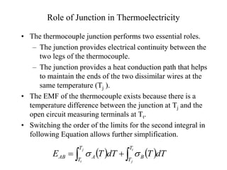
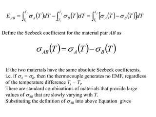
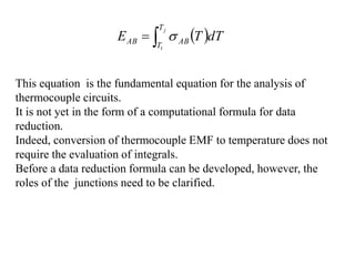
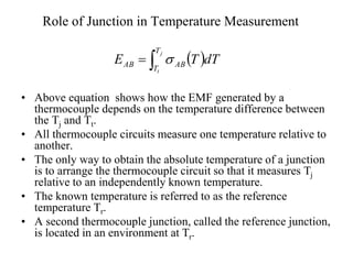
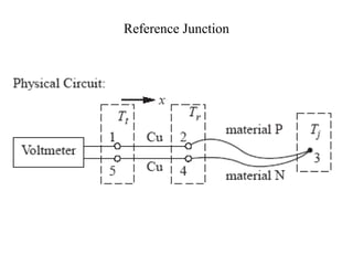
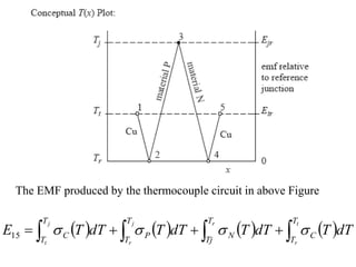
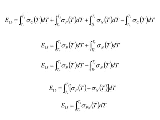
The document discusses thermoelectric effects and how thermocouples measure temperature. It explains that thermocouples use the Seebeck effect where two dissimilar metals generate a voltage proportional to the temperature difference between their junctions. A reference junction at a known temperature is used to determine the absolute temperature. Standard thermocouple types are identified and calibration involves fitting curves to voltage-temperature data rather than directly evaluating integrals from the fundamental thermocouple equation.

1. Thermo Electric Effects & Temperature
Measurement
P M V Subbarao
Professor
Mechanical Engineering Department
Selection of an Instrument for a Need….

2. Thermoelectric Phenomena
• Electrically conductive materials exhibit three types of
thermoelectric phenomena:
• the Seebeck effect,
• the Thompson effect, and
• the Peltier effect.
• The use of thermocouples is based on thermoelectric
phenomenon discovered by Thomas Seebeck in 1821.
• When any two metals are connected together, a voltage is
developed which is a function of the temperatures of the
junctions and (mainly) the difference in temperatures.
• It was later found that the Seebeck voltage is the sum of two
effects: the Peltier effect, and the Thompson effect.
• The Peltier effect explains a voltage generated in a junction of
two metal wires.
• The Thompson effect explains a voltage generated by the
temperature gradient in the wires.

3. EMF Relationships for Thermocouples
• Practical exploitation of the Seebeck effect to measure temperature
requires a combination of two wires with dissimilar Seebeck
coefficients.
• The name thermocouple reflects the reality that wires with two
different compositions are combined to form a thermocouple
circuit.
Apply  
dT
dE
T 
 To above figure

4.  dT
T
dE 

The EMF generated in material A between the junction at Tt and the
junction at Tj is
 


j
t
T
T
A
tj
A dT
T
E 
,
Applying above Equation to consecutive segments of the circuit gives
   

 

t
j
j
t
T
T
B
T
T
A
AB dT
T
dT
T
E 


5. Basics of Thermocouple Thermometry
• A is the absolute Seebeck coefficient of material A, and B is the
absolute Seebeck coefficient of material B.
• The order of integration is specified by moving continuously
around the loop: from the terminal to the junction, and back to the
terminal.
• The position of the junction around the thermocouple circuit is
identified by the x coordinate.
• For the purpose of analyzing thermocouple circuits, the physical
length of wire is immaterial.
• Accordingly, x should be thought of an indicator of position only,
not a measure of distance.
• Notice that the value of EAB in above Equation is due to integrals
along the length of the thermocouple elements.
• This leads to an essential and often misunderstood fact of
thermocouple thermometry:

6. Misconception in Thermoelectricity
The EMF generated by the Seebeck effect is due to the temperature
gradient along the wire.
The EMF is not generated at the junction between two dissimilar wires.

7. Role of Junction in Thermoelectricity
• The thermocouple junction performs two essential roles.
– The junction provides electrical continuity between the
two legs of the thermocouple.
– The junction provides a heat conduction path that helps
to maintain the ends of the two dissimilar wires at the
same temperature (Tj ).
• The EMF of the thermocouple exists because there is a
temperature difference between the junction at Tj and the
open circuit measuring terminals at Tt.
• Switching the order of the limits for the second integral in
following Equation allows further simplification.
   

 

t
j
j
t
T
T
B
T
T
A
AB dT
T
dT
T
E 


8.        
 


 



j
t
j
t
j
t
T
T
B
A
T
T
B
T
T
A
AB dT
T
T
dT
T
dT
T
E 



Define the Seebeck coefficient for the material pair AB as
     
T
T
T B
A
AB 

 

If the two materials have the same absolute Seebeck coefficients,
i.e. if A = B, then the thermocouple generates no EMF, regardless
of the temperature difference Tj − Tt.
There are standard combinations of materials that provide large
values of AB that are slowly varying with T.
Substituting the definition of AB into above Equation gives

9.  


j
t
T
T
AB
AB dT
T
E 
This equation is the fundamental equation for the analysis of
thermocouple circuits.
It is not yet in the form of a computational formula for data
reduction.
Indeed, conversion of thermocouple EMF to temperature does not
require the evaluation of integrals.
Before a data reduction formula can be developed, however, the
roles of the junctions need to be clarified.

10. Role of Junction in Temperature Measurement
• Above equation shows how the EMF generated by a
thermocouple depends on the temperature difference between
the Tj and Tt.
• All thermocouple circuits measure one temperature relative to
another.
• The only way to obtain the absolute temperature of a junction
is to arrange the thermocouple circuit so that it measures Tj
relative to an independently known temperature.
• The known temperature is referred to as the reference
temperature Tr.
• A second thermocouple junction, called the reference junction,
is located in an environment at Tr.
 


j
t
T
T
AB
AB dT
T
E 

11. Reference Junction

12. The EMF produced by the thermocouple circuit in above Figure
       



 



t
r
r
j
r
j
t
T
T
C
T
Tj
N
T
T
P
T
T
C dT
T
dT
T
dT
T
dT
T
E 



15

13.        



 



r
t
r
j
r
j
t
T
T
C
T
Tj
N
T
T
P
T
T
C dT
T
dT
T
dT
T
dT
T
E 



15
   

 

r
j
r
T
Tj
N
T
T
P dT
T
dT
T
E 

15
   

 

j
j
r
T
Tr
N
T
T
P dT
T
dT
T
E 

15
   
 
 

j
r
T
T
N
P dT
T
T
E 

15
 


j
r
T
T
PN dT
T
E 
15

14. Material EMF versus Temperature
With reference to
the characteristics
of pure Platinum
emf
Temperature
Chromel
Iron
Copper
Platinum-Rhodium
Alumel
Constantan

15. Standard Thermocouples
• The ASTM identifies eight standard types of thermocouples.

16. Making of Thermocouple Junction
• Any time a pair of dissimilar wires is
joined to make a circuit and a thermal
gradient is imposed, an emf voltage
will be generated.
• Twisted, soldered or welded junctions
are acceptable. Welding is most
common.
• Keep weld bead or solder bead
diameter within 110-115% of wire
diameter
• Welding is generally quicker than
soldering but both are equally
acceptable

17. Thermocouple temperature vs.Voltage graph

18. Seebeck coefficient vs. Temperature

19. Standard Calibration Setup
Ice-point
The result of the calibration is a table of EMF versus T values.
The integral is never directly evaluated.
Instead a polynomial curve fit to the calibration data gives:
  n
j
n
j
j
j
j T
b
T
b
T
b
b
T
F
E 




 .....
2
2
1
0
0