Mechanics of Materials Lab Manual C20.pdf

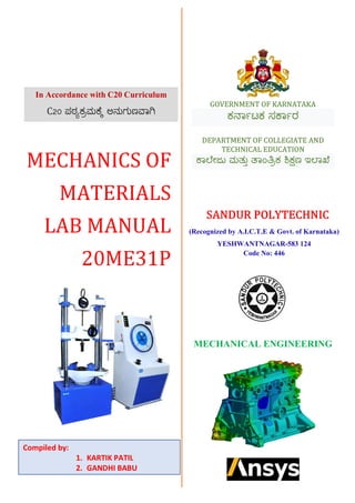
GOVERNMENT OF KARNATAKA
ಕ ಾ ಟಕ ಸ ಾ ರ
DEPARTMENT OF COLLEGIATE AND
TECHNICAL EDUCATION
ಾ ೇಜು ಮತು ಾಂ ಕ ಣ ಇ ಾ ೆ
(Recognized by A.I.C.T.E & Govt. of Karnataka)
YESHWANTNAGAR-583 124
Code No: 446
MECHANICAL ENGINEERING
Compiled by:
1. KARTIK PATIL
2. GANDHI BABU
In Accordance with C20 Curriculum
C20 ಪಠ ಕ ಮ ೆ ಅನುಗುಣ ಾ

VISION OF INSTITUTE
To make every student of the Sandur Polytechnic well educated, trained and globally
competitive for meaningful contribution to the socio-economic development of the Country.
MISSION
To provide high quality technical education and training at affordable cost to boys and girls, to
develop skills and enable them acquire engineering, entrepreneurial and leadership qualities.
VISION OF DEPARTMENT
To develop highly competent Engineers with advanced technical skills and adept in modern
Mechanical process, along with good leadership qualities and work ethics.
MISSION
1. To impart Knowledge of Basic science and Mechanical Engineering skills through effective
and efficient training.
2. To provide students with value-based Education and create an environment of academic
excellence with good leadership qualities and professional ethics.
3. To ensure development of students in other important aspects like Life skills, environment
awareness and social conduct, and to make them useful to the society and industries.
PROGRAM OUTCOMES
1. Basic and Discipline specific knowledge: Apply knowledge of basic mathematics, science and
engineering fundamentals and engineering specialization to solve the engineering problems.
2. Problem analysis: Identify and analyze well-defined engineering problems using codified
standard methods.
3. Design/ development of solutions: Design solutions for well-defined technical problems and
assist with the design of systems components or processes to meet specified needs.
4. Engineering Tools, Experimentation and Testing: Apply modern engineering tools and
appropriate technique to conduct standard tests and measurements.
5. Engineering practices for society, sustainability and environment: Apply appropriate
technology in context of society, sustainability, environment and ethical practices.
6. Project Management: Use engineering management principles individually, as a team member
or a leader to manage projects and effectively communicate about well-defined engineering
activities.
7. Life-long learning: Ability to analyze individual needs and engage in updating in the context of
technological changes.

Engineering Mechanics Exercises
Sandur Polytechnic Department of Mechanical Engineering Page: 2.1
EXERCISE: 01 DATE:
RESOLUTION OF FORCES BY GRAPHICAL METHOD
AIM: Resolution of coplanar concurrent forces by Graphical method to find resultant force for the
given system of force.
TOOLS REQUIRED:
1. Engineering instrument Box
2. Papers A4
3. Mini Drafter and Drawing Clips
THEORY: Resultant of Several Coplanar Concurrent Forces
To determine the resultant of a number of coplanar concurrent forces any of the following two
methods may be used:
1. Graphical method (Polygon law of forces)
2. Analytical method (Principle of resolved parts).
Polygon law of forces. If a number of coplanar concurrent forces, acting simultaneously on a body
are represented in magnitude and direction by the sides of a polygon taken in order, then their
resultant may be represented in magnitude and direction by the closing side of a polygon, taken in
the opposite order.
If the forces P1, P2, P3, and P4 acting simultaneously on a particle O be represented in
magnitude and direction by the sides oa, ab, bc and cd of a polygon respectively, their resultant is
represented by the closing side do in the opposite direction as shown in Fig. (b).

PROCEDURE:
1. Construction of space diagram (position diagram). It means the construction of a diagram
showing the various forces (or loads) along with their magnitude and lines of action.
2. Use notations. All the forces in the space diagram are named by notations. It is a convenient
method in which every force (or load) is named by capital letter, placed on its either side in
the space diagram.
3. Construction of vector diagram (force diagram). It means the construction of a diagram
starting from a convenient point and then go on adding all the forces vectorially one by one
(keeping in view the directions of the forces) to some suitable scale. Now the closing side of
the polygon, taken in opposite order, will give the magnitude of the resultant force (to the
scale) and its direction.
RESULT: The magnitude and direction of Resultant force for the given space diagrams are found.

EXERCISE:02 DATE:
VERIFICATION OF LAMI’S THEOREM
AIM: To verify Lami's Theorem with the help of Gravesand’s apparatus.
TOOLS AND EQUIPMENT USED
1. Gravesand’s apparatus,
2. Detachable pulley,
3. Rings with three strings,
4. Slotted weights and hangers
THEORY:
As we know when a particle is acted upon by a number of forces. The resultant force will
produce the same effect as produced by all the given forces. If the resultant of a number of
forces, acting on a particle is zero, the particle will be in equilibrium. Such a set of forces, whose
resultant is zero, are called equilibrium forces.
The force, which brings the set of forces in equilibrium is called an equilibrant. As a
matter of fact, the equilibrant is equal to the resultant force in magnitude, but opposite in
direction.
Lami's Theorem is related to the
magnitudes of concurrent, coplanar, and
non-collinear forces that maintain an
object in static equilibrium.
Statement: “When three forces acting at a point are in equilibrium, then each force is
proportional to the sine of the angle between the other two forces”
In the mathematical or equation form, it is expressed as,

TABULAR COLUMN
Trail
No.
Forces in ‘gm’
Angle between each force
in ‘degree’
Ratios
P Q R α β 
𝑃
𝑠𝑖𝑛 ∝
𝑄
𝑠𝑖𝑛 𝛽
𝑅
𝑠𝑖𝑛 𝛾
1
2
3
PROCEDURE
1. Set the board in a vertical plane and fix the paper sheet with drawing pins/clips.
2. Pass a thread over two pulleys.
3. Take a second thread and tie the middle of this thread to the middle of first thread.
4. Attach weight hangers to the free ends of the threads as shown in Fig.
5. Place the weights in such a manner that the knot comes approximately in the centre of the
paper.
6. Take the table lamp and place Infront of threads and turn ON.
7. Mark the points by keeping the eye shadow image of the threads without disturbing the system.
8. Remove the paper from the board and produce the lines to meet at O.
9. Measure the angle α, β and .
10. Verify the relationship.
11. Repeat the same for different load trails.
CALCULATION
RESULT: Lami’s Theorem verified successfully using Gravesand’s apparatus

Mechanical Testing for Materials Experiments and practice
IMPORTANCE OF MATERIAL TESTING
Materials testing and characterization is carried out to understand the fundamental
properties of a material when subjected to service and environmental loading and operating
conditions. Testing helps us to understand and quantify whether a specific material is suitable to a
particular application. For mechanical testing of materials there are generally two classes of
testing machines;
1. Non destructive testing
2. Destructive testing
Non-destructive testing
Non-destructive testing or (NDT) is a wide group of analysis techniques used in science
and technology industry to evaluate the properties of a material, component or system without
causing damage to the specimen. The five most frequently used NDT methods are
1. Magnetic-particle,
2. Liquid dye penetrant,
3. Radiographic,
4. Ultrasonic
5. Visual testing
Destructive testing
In destructive testing (or destructive physical analysis, DPA) tests are carried out to the
specimen's failure, in order to understand a specimen's performance or material behaviour under
different loads. Some types of destructive testing:
1. Stress tests
2. Crash tests
3. Hardness tests
4. Metallographic tests

Some of the important mechanical properties of the metals are
1. Brittleness: The tendency of material to fracture or fail upon the application of a relatively
small amount of force, impact or shock.
2. Creep: When a metal is subjected to a constant force at a high temperature below its yield
point, for a prolonged period of time, it undergoes a permanent deformation.
3. Ductility: Ductility is the property by which a metal can be drawn into thin wires. It is
determined by percentage elongation and percentage reduction in the area of metal.
4. Elasticity: Elasticity is the tendency of solid materials to return to their original shape
after being deformed.
5. Fatigue: Fatigue is the material weakening or breakdown of equipment subjected to stress,
especially a repeated series of stresses.
6. Hardness: Hardness is the ability of material to resist indentation, penetration and
scratching caused by an external force.
7. Malleability: Malleability is the property by which a metal can be rolled into thin sheets.
8. Plasticity: Plasticity is the property by which a metal retains its deformation permanently,
when the external force applied on it is released.
9. Resilience: Resilience is the ability of metal to absorb energy elastically and resist soft
and impact load.
10. Stiffness: Stiffness is the ability of metal to resist deformation under stress.
11. Toughness: Ability of a material to absorb energy and plastically deform without
fracturing.

Universal testing machine
The loading unit
The loading unit consists of a robust base at the centre of which is fitted the main cylinder
and piston. A rigid frame consisting of the lower table, the upper cross head and the two straight
columns is connected to this piston through a ball and socket joint. A pair of screwed columns
mounted on the base pass through the main nuts to support the lower cross-head. This cross head
is moved up or down when the screwed columns are rotated by a geared motor fitted to the base.
Each cross-head has a tapering slot at the centre into which are inserted a pair of racked
jaws. These jaws are moved up or down by the operating handle on the cross-head face and is
intended to carry the plate (grip) jaws for the tensile test specimen.
The control panel
The control panel contains the hydraulic power unit, the load measuring unit and the control
devices.
The Hydraulic Power Unit
The Hydraulic Power Unit consists of an oil pump driven by an electric motor and a sump
for the hydraulic oil. The pump is of the reciprocating type, having a set of plungers which assures
a continuous non-pulsating oil flow into the main cylinder for a smooth application of the test load
on the specimen.

The Load Measuring Unit
The load measuring unit, in essence is a pendulum dynamometer unit. It has a small
cylinder in which a piston moves in phase with the main piston under the same oil pressure. A
simple pendulum connected with this small piston by a pivot lever thus deflects in accordance
with the load on the specimen and the pivot ratio. This deflection is transmitted to the load pointer
which indicates the test load on the dial.
Control Devices
The Electric Control Devices are in the form of four switches set on the panel face. The
upper and lower push switches are for moving the lower cross-head up and down respectively.
The remaining two are the ON and OFF switches for the hydraulic pump.
The Hydraulic Control Devices are a pair of control valves set on the table or the control
panel. The right control valve is the inlet valve. It is a pressure compensated flow control valve
and has a built-in overload relief valve. If this valve is in the closed position, while the hydraulic
system is on, oil flows back into the sump. Opening of the valve now, cause the oil to flow into
the main cylinder in a continuous non-pulsating manner. The left control valve is the return valve.
If this valve is in the closed position, the oil pumped into the main cylinder causes the main piston
to move up. The specimen resists this, movement, as soon as it gets loaded up. Oil pressure inside
the main cylinder (and elsewhere in the line) then starts growing up until either the specimen
breaks or the load reaches the maximum value of the range selected. A slow opening of this valve
now causes the oil to drain back into the sump and the main piston to descent.

EXPT: 01 DATE:
TENSILE TEST (ASTM E8- METALS)
AIM: Determination of yield stress, ultimate stress, breaking stress, percentage reduction
in area, percentage elongation, young’s modulus by conducting tension test on mild steel
on universal testing machine. Draw Load vs. Deformation curve.
Theory
In a tensile test of mild steel specimen is subjected to gradually pull in a testing
machine until it breaks and at each and every increment of load the corresponding
deformation is noted. Two points, called gauge points, are marked on the central portion. The
distance between these points, before the application of the load, is called gauge length of the
specimen. The extensions are measured by an instrument called an extensometer.
Observations
1. Maximum load selected :_________________________ KN
2. Least count of Load dial :_________________________ KN
3. Least count of extensometer :_________________________mm
4. Material used :_________________________
5. Initial diameter of specimen Di :_________________________mm
6. Initial length of specimen Li :_________________________mm
7. Gauge length of specimen 7×d :_________________________mm
8. Final length of specimen Lf :_________________________mm
9. Final diameter of specimen Df :_________________________mm
10. Ultimate load :_________________________KN

11. Yield-load :_________________________KN
12. Breaking load :_________________________KN
Equipments required
1. UTM machine 2. Extensometer
3. Scale and calipers 4. Ball peen hammer and dot punch
Tabular column
Load in
(KN)
Deformation
(Div)
Deformation
ΔL (mm)
Engg. Stress
(KN/mm2
)
Engg.
Strain
Young’s
modulus
(KN/mm2
)
% of
Elongation
Procedure
1. Initial dimensions of specimen are measured using scale and vernier caliper.
2. Two points, called gauge points, are marked on the central portion. The distance between
these points, before the application of the load, is called gauge length of the specimen.
3. Machine is switched ON and suitable load is selected.
4. The middle cross head is lowered to fix the specimen in jaw.
5. Now middle cross head is raised and other end of specimen is gripped in upper cross head
jaws.
6. Hydraulic pump is switched ON; return valve is completely closed and is allowed to run
for 2 min.
7. Hydraulic pressure is applied by slightly opening other valve.
8. The extensions of the gauge length and the values of the corresponding loads are required
at frequent intervals and are continuous until specimen fails.
9. Note down final length and diameter of specimen.
10. Release pressure after completion of experiment by opening release valve.
11. Readings are tabulated and graph is plotted load vs. elongation.

Calculation
1. Initial area of specimen (Ai )
𝜋×𝐷𝑖2
4
mm2
2. Final area of specimen (Af )
𝜋×𝐷𝑓2
4
mm2
3. Deformation= Deformation in Div× Least count of extensometer_________mm
4. Engineering Stress=
Load
Ai
in KN/mm2
5. Engineering Strain=
ΔL
Li
6. Yield stress:
Yield load
Ai
KN/mm2
7. Ultimate stress:
Ultimate load
Ai
KN/mm2
8. Breaking stress:
Breaking load
Ai
KN/mm2
9. Young’s modulus:
𝑆𝑡𝑟𝑒𝑠𝑠
strain
KN/mm2
(From the graph within elastic limits)
10. Percentage of elongation (ductility)=
Lf−Li
Li
× 100
11. Percentage of reduction in area=
Ai−Af
Ai
× 100
Result: Experiment is carried and following characteristics are found
1. Yield stress:
2. Ultimate stress:
3. Breaking stress:
4. Percentage of reduction in area:
5. Percentage of elongation:

EXPT: 02 DATE:
COMPRESSION TEST
AIM: Find out Compressive Strength of WOOD using Universal Testing Machine.
Draw Load vs. Deformation curve
Theory
A bi-modulus material, which young’s modulus is different from the compression one
along the same direction, is widely used in engineering, e.g., concrete, cast iron, etc. Ductile
materials attain a Bulge or a Barrel shape after reaching the maximum Compression load. No
fracture takes place and there is change in cross section and compression value remains the same
on reaching the maximum load. For brittle materials, there will be no change in the cross-sections
or height of the specimen due to the compression load. On reaching the maximum compression
load, the specimen suddenly fractures.
However, there are certain practical difficulties which may induce error in this test.
1. Difficulty in applying truly axial load.
2. There is always a tendency of the specimen to bend in addition to Contraction i.e. buckle.
To avoid these errors, usually the specimen for this test shall be short in length (not more
than 2 time the area)
Equipments required
1. UTM machine
2. Extensometer
3. Scale & calipers

Observations
1. Maximum load selected :_____________________________KN
2. Least count of Load dial :_____________________________KN
3. Least count of extensometer :_____________________________KN
4. Material used :_____________________________
5. Initial length of specimen Li :_____________________________mm
6. Initial breadth of specimen Wi :_____________________________mm
7. Initial height of specimen Hi :_____________________________mm
8. Final length of specimen Lf :_____________________________mm
9. Final breadth of specimen Wf :_____________________________mm
10. Final height of specimen Hf : _____________________________mm
11. Ultimate load :_____________________________KN
12. Breaking load :_____________________________KN
Procedure
1. Initial dimensions of specimen are measured using scale and caliper.
2. Fix compression pads to the machine and place specimen in between pads across the grain.
3. Machine is switched ON and suitable load is selected. Fix the extensometer and adjust the
dial of extensometer at zero.
4. Keep speed of machine uniform. Record maximum load point, point of breaking of
specimen.
5. Remove the specimen from machine and study the fracture observes type of fracture.
6. Measure dimensions of tested specimen. Readings are tabulated and graph is plotted.

Calculation
1. Initial area of specimen Ai = Li ×Wi _______________ mm2
2. Final area of specimen Af= Lf ×Wf ________________ mm2
3. Deformation in mm= Deformation in Div× Least count of extensometer_____ mm
4. Compressive stress=
𝐿𝑜𝑎𝑑
𝐴𝑖
KN/mm2
5. Compressive strain=
ΔH
Hi
6. Ultimate stress:
Ultimate load
Ai
__________________ KN/mm2
7. Breaking stress:
Breaking load
Ai
__________________ KN/mm2
Compressive stress
Compressive strain
KN/mm2
(From the graph with in elastic limits)
9. Percentage of increase in area
Af−Ai
Af
×100____________________
10. Percentage of reduction in height=
Hi−Hf
Hi
× 100__________________
Tabular column
Load in
(KN)
Deformation
(Div)
Deformation
ΔH (mm)
Engg. Stress
(KN/mm2
)
Engg.
Strain
Young’s
modulus
(KN/mm2
)
% of
increase
in area
1. Ultimate stress:
2. Breaking stress:
3. Percentage of reduction in height:
4. Percentage of increase in area:

EXPT: 03 DATE:
BENDING TEST
AIM: Find out Bending Strength of WOOD using Universal Testing Machine. Draw Load vs.
Deformation curve.
Theory
If a beam is simply supported at the ends and carries a concentrated load at the center, the
beam bends concave upwards. The distance between the original position of the beam and its
position after bending is different at different points (fig) along the length if the beam, being
maximum at the center in this case. This difference is called ‘deflection’.
We know that Bending equation:
M
I
=
Fb
Y
=
E
R
Where,
M= Bending moment
I= Moment of inertia
Fb= Bending stress
y= Depth of neutral axis
E= Young’s modulus
R= Radius of curvature
Equipments required
1. UTM machine 2. Extensometer 3. Scale & calipers
Procedure
1. Adjust the supports along the UTM bed so that they are symmetrically with respect to the
length of the bed.
2. Place the beam on the knife- edges so as to project equally beyond each support. See that
the load is applied at the center of the beam.
3. Fix the extensometer and adjust the dial of extensometer at zero.
4. Go on taking reading applying load in steps each time till the specimen fails.
5. Draw a graph between load (W) and deflection (dl).
6. Calculate the bending stresses for different loads using relation.

Observations
1. Maximum load selected :____________________________KN
2. Least count of Load dial : ____________________________mm
3. Least count of extensometer : ____________________________mm
4. Material used : ____________________________
5. Length of specimen (L) : ____________________________mm
6. Breadth of specimen (b) : ____________________________mm
7. Depth of specimen (d) : ____________________________mm
8. Depth of neutral axis (y)=
𝑑
2
: ____________________________mm
9. Moment of inertial (I) =
bd3
12
: ____________________________mm4
10. Ultimate load : ____________________________KN
11. Breaking load : ____________________________KN

Tabular column
Load
(W)
in KN
Deformation
(Div)
Deformation (Δ)
(mm)
Bending
Moment
KN-mm
Bending
Stress
KN/mm2
Young’s
Modulus (E)
KN/mm2
Calculation
1. Deformation in mm= Deformation in Div× Least count of extensometer_____ mm
2. Bending Moment ‘M’=
W×L
4
in KN-m
3. Bending Stress Fb=
M×y
I
in KN/mm2
4. Young’s modulus E=
WL3
48×Δ×I
KN/mm2
(From the graph within elastic limit)
1. Bending strength:

Awareness about using ANSYS and Familiarization
Computer-aided engineering (CAE)
It is the broad usage of computer software to aid in engineering analysis tasks. It includes
1. Finite element analysis (FEA),
2. Computational fluid dynamics (CFD), and
3. Optimization.
The elements of Computer aided Engineering
Three phases in any Computer-Aided Engineering task
In general, there are three phases in any computer-aided engineering task:
1. Pre-processing – defining the model and environmental factors to be applied to it. (typically,
a finite element model, but facet, voxel and thin sheet methods are also used)
2. Analysis solver (usually performed on high powered computers)
3. Post-processing of results (using visualization tools)
CAE areas covered include
1. Stress analysis on components and assemblies using Finite Element Analysis (FEA)
2. Thermal and fluid flow analysis Computational fluid dynamics (CFD)
3. Multibody dynamics (MBD) and Kinematics
4. Analysis tools for process simulation for operations such as casting, moulding, and die press
forming.
5. Optimization of the product or process.

Finite Element Analysis
FEA: The mathematical equations are applied to create a simulation. This simulation is used
to provide a structural analysis of how a particular product or design would react under stress in the
real world.
The simulation breaks down the entire model into smaller elements within a mesh, which
engineers use to test how the different elements of a design.
The finite element method works by breaking down a large problem into smaller problems
called “finite elements.” Using this method, engineers can test each element’s behaviour using
computer-aided engineering software.
Nodes and Elements in Finite Element Analysis
In FEA, you divide your model into small pieces. Those are called Finite Elements (FE). Those
Elements connect all characteristic points (called Nodes)
The 1D element is just a line connecting two nodes.

2D elements are usually triangular (TRI) and Quadrilateral (QUAD) in shape.
3D solid elements can be based on triangles and quads as well, those will produce the
epitome of Finite Elements – TET and HEX elements:
Element properties:
1. Straight or curved one-dimensional elements. This type of element is suitable for modelling
cables, braces, trusses, beams, stiffeners, grids and frames. Straight elements usually have
two nodes, one at each end, while curved elements will need at least three nodes including the
end-nodes. The elements are positioned at the centroidal axis of the actual members.

2. Two-dimensional elements that resist only in-plane forces by membrane action. They may
have a variety of shapes such as flat or curved triangles and quadrilaterals. Nodes are usually
placed at the element corners.
3. Three-dimensional elements for modelling 3-D solids such as machine components. Nodes
are placed at the vertexes and possibly in the element faces or within the element.

ANSYS analysis has three distinct steps
1. Build the model.
2. Apply loads and obtain the solution.
3. Review the results.
Building a Model
Building a finite element model requires more of an ANSYS.
1. Specify a jobname and analysis title.
2. The PREP7 pre-processor to define the element types, element real constants, material
properties, and the model geometry.
Specifying a Jobname and Analysis Title
This task is not required for an analysis, but is recommended.
Defining the Jobname
The jobname is a name that identifies the ANSYS job. When we define a jobname for
an analysis, the jobname becomes the first part of the name of all files the analysis creates.
The extension or suffix for these files' names is a file identifier such as .DB. By using
a jobname for each analysis, you insure that no files are overwritten. If you do not specify a
jobname, all files receive the name FILE or file, depending on the operating system.

Command(s): /FILNAME
GUI: Utility Menu>File>Change Jobname
The element type determines, among other things
The degree-of-freedom set (which in turn implies the discipline-structural, thermal, magnetic,
electric, quadrilateral, brick, etc.). Whether the element lies in two-dimensional or three-dimensional
space. For example, BEAM4, has six structural degrees of freedom (UX, UY, UZ, ROTX, ROTY,
ROTZ), is a line element, and can be modelled in 3-D space. PLANE77 has a thermal degree of
freedom (TEMP), is an eight-node quadrilateral element, and can be modelled only in 2-D space.

Defining Element Real Constants
Element real constants are properties that depend on the element type, such as cross-sectional
properties of a beam element. For example, real constants for BEAM3, the 2-D beam element, are
area (AREA), moment of inertia (IZZ), height (HEIGHT), shear deflection constant (SHEARZ),
initial strain (ISTRN), and added mass per unit length (ADDMAS).
Not all element types require real constants, and different elements of the same type may have
different real constant values. As with element types, each set of real constants has a reference
number, and the table of reference number versus real constant set is called the real constant table.
While defining the elements, you point to the appropriate real constant reference number using the
REAL command (Main Menu> Pre-processor>Create>Elements>Elem Attributes).
Defining Material Properties

Most element types require material properties. Depending on the application, material
properties may be: Linear or nonlinear, Isotropic, orthotropic, or anisotropic Constant temperature or
temperature-dependent
As with element types and real constants, each set of material properties has a material
reference number. The table of material reference numbers versus material property sets is called the
material table.
Main Menu> Pre-processor> Material Props> Material Models.
Creating the Model Geometry
The next step in an analysis is generating a finite element model-nodes and elements-that
adequately describes the model geometry.
Apply Loads and Obtain the Solution
In this step, you use the SOLUTION processor to define the analysis type and analysis
options, apply loads, specify load step options, and initiate the finite element solution. You also can
apply loads using the PREP7 pre-processor.

Applying Loads
The word loads as used in this manual includes boundary conditions (constraints,
supports, or boundary field specifications) as well as other externally and internally applied
loads. Loads in the ANSYS program are divided into six categories:
1. DOF Constraints
2. Forces
3. Surface Loads
4. Body Loads
5. Inertia Loads
6. Coupled-field Loads
Initiating the Solution
To initiate solution calculations, use either of the following:
Command(s): SOLVE

GUI: Main Menu>Solution>Current LS
When you issue this command, the ANSYS program takes model and loading information
from the database and calculates the results. Results are written to the results file (Jobname. RST,
Jobname. RTH, Jobname. RMG, or Jobname. RFL) and also to the database. The only difference is
that only one set of results can reside in the database at one time, while you can write all sets of
results (for all sub steps) to the results file.
Review the Results
Once the solution has been calculated, you can use the ANSYS postprocessors to review the results.
General Steps
Step 1: Ansys Utility Menu
File – clear and start new – do not read file – ok
File – change job name – enter new job name – xxxx – ok
File – change title – enter new title – yyy – ok
Step 2: Ansys Main Menu – Preferences select – STRUCTURAL - ok
Step 3: Pre-processor
Element type – select type of element from the table and the required options
Real constants – give the details such as thickness, areas, moment of inertia, etc.
required depending on the nature of the problem.
Material Properties – give the details such as Young’s modulus, Poisson’s ratio etc.
depending on the nature of the problem.
Modelling – create the required geometry such as nodes elements, area, volume by using the
appropriate options.
Generate – Elements/ nodes using Mesh Tool if necessary (in 2D and 3D problems)
Step 6: Apply boundary conditions/loads such as DOF constraints, Force/Momentum, Pressure etc.
Solution – Solve the problem
Step 8: General Post Processor – plot / list the required results.
Step 9: Plot ctrls – animate – deformed shape – def+undeformed-ok
Step 10: To save the solution ANSYS tool bar- save,,,,model

Validate Bending Equation using ANSYS simulation
Sandur Polytechnic Department of Mechanical Engineering Page: 3. 1
EXPT: 11 DATE:
Aim: To validate the bending equation using ANSYS software and compare the results with analytical
calculation.
Problem descriptions:
Compute shear force and bending moment diagrams for the beams as shown below. Also find
Bending stress induced in the beam for the given data.
E= 210Gpa, μ=0.3 and C/s (b=0.2m & d=0.3m) Rectangular Beam.
Cantilever Beam Shear Force Calculations
At 4 = -10 kN
At 3 = (-10) + (-20) = -30 kN
At 2 = (-10) + (-20) + (-30) = -60 kN
At 1 = -60 kN
Bending moment calculations
At 4 = (-10 ×0) = 0 kN-m
At 3 = (-10 ×2) + (-20 ×0) = -20 kN-m
At 2 = (-10 ×4) + (-20 ×2) + (-30 ×0) = -80 kN-m
At 1 = (-10 ×5) + (-20 ×3) + (-30 ×1) = -140 kN-m
Bending stress calculation
Moment of inertia(I) = =
. × .
= 4.5×10-4
m4
Depth of neutral axis (y)= =
.
= 0.15m
Bending Stress (σb) =
×
=
× .
4.5E−4
= -46,666.67KN/m2

Comparison Table
Particulars
Analytical results ANSYS results
Maximum Minimum Maximum Minimum
Shear force
Bending Moment
Bending stress
Result: The analysis of the beam was carried out using the Ansys simulation and the software results
were compared with theoretical or analytical results.
Conclusion: Ansys simulation and the software results are near to theoretical or analytical results.

EXPT: 12 DATE:
calculation.
At 3 = 0 N
At 2 = 0 N
Upto 1= (-120×1.2) = -144 N
At 3 = 0 N-m
At 2 = 0 N-m
At 1 = -120 ×1.2×
.
= -86.4 N-m
. × .
= 4.5×10-4
m4
.
= 0.15m
×
=
. × .
4.5E−4
= -28,800 N/m2