Measures for Central Tendency/location/averages

1. Measures of Central Tendency
or
Measures of Location
or
Measures of Averages
-By Dr Abhishek Dondapati

2. INVESTIGATION
Data Colllection
Data Presentation
Tabulation
Diagrams
Graphs
Descriptive Statistics
Measures of Location
Measures of Dispersion
Measures of Skewness &
Kurtosis
Inferential Statistiscs
Estimation Hypothesis
Testing
Ponit estimate
Inteval estimate
Univariate analysis
Multivariate analysis

3. Descriptive Statistics
Descriptive statistics are brief informational coefficients that
summarize a given data set, which can be either a representation of
the entire population or a sample of a population.
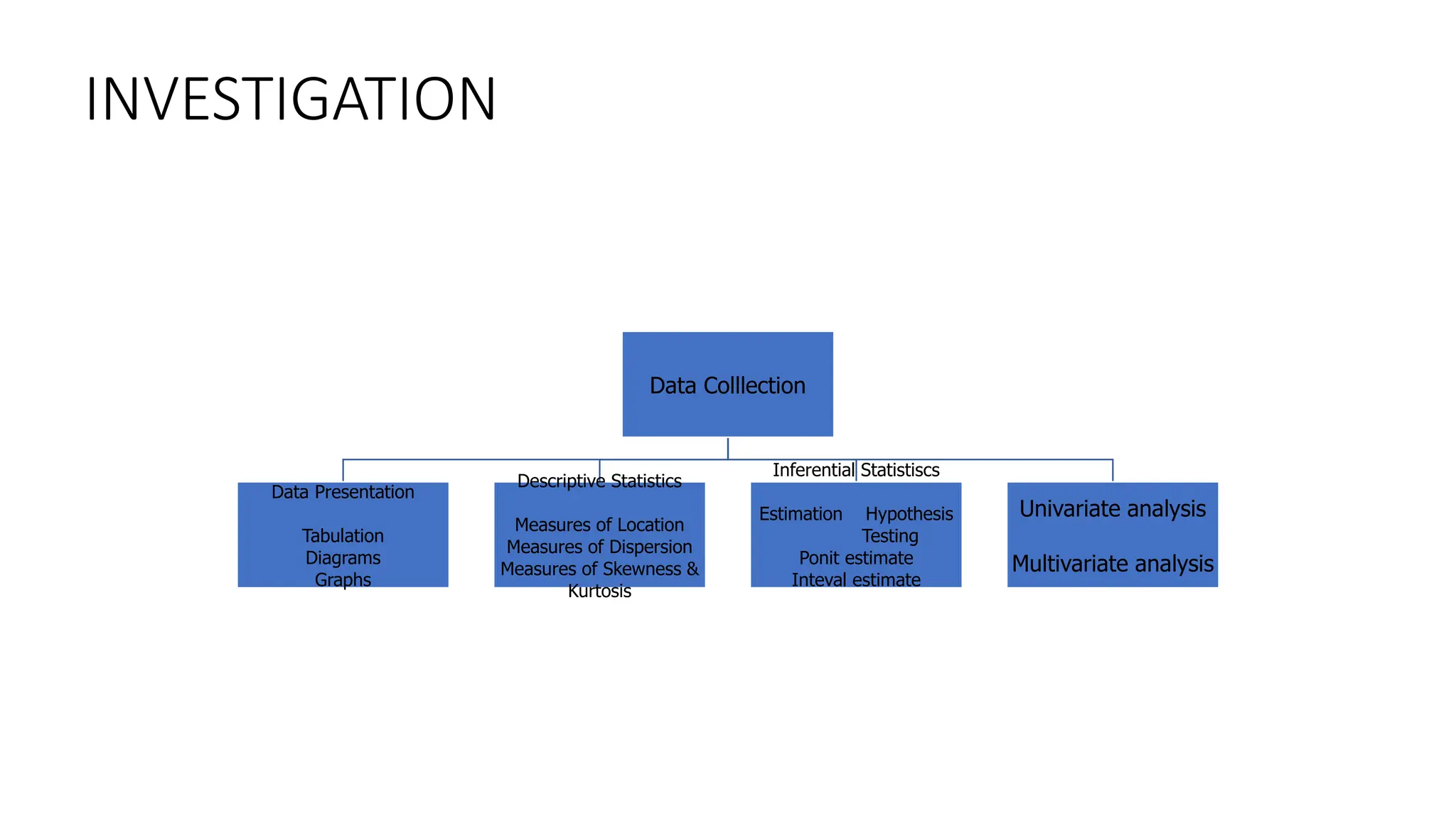
Descriptive statistics are broken down into measures of central
tendency and measures of variability (spread).
Measures of central tendency include the mean, median, and mode,
while measures of variability include standard deviation, variance,
minimum and maximum variables, kurtosis, and skewness.

4. Measures of central tendency
• Central Tendency is defined as "middle value" or
typical value of data, which represents the whole data
set
• It gives us an idea of the "value" around which all the
observations in a data set appear to concentrate
• The most important and frequently used measures of
central tendency are mean, median and mode

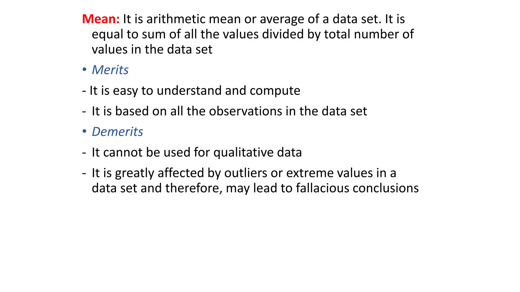
5. Mean: It is arithmetic mean or average of a data set. It is
equal to sum of all the values divided by total number of
values in the data set
• Merits
- It is easy to understand and compute
- It is based on all the observations in the data set
• Demerits
- It cannot be used for qualitative data
- It is greatly affected by outliers or extreme values in a
data set and therefore, may lead to fallacious conclusions

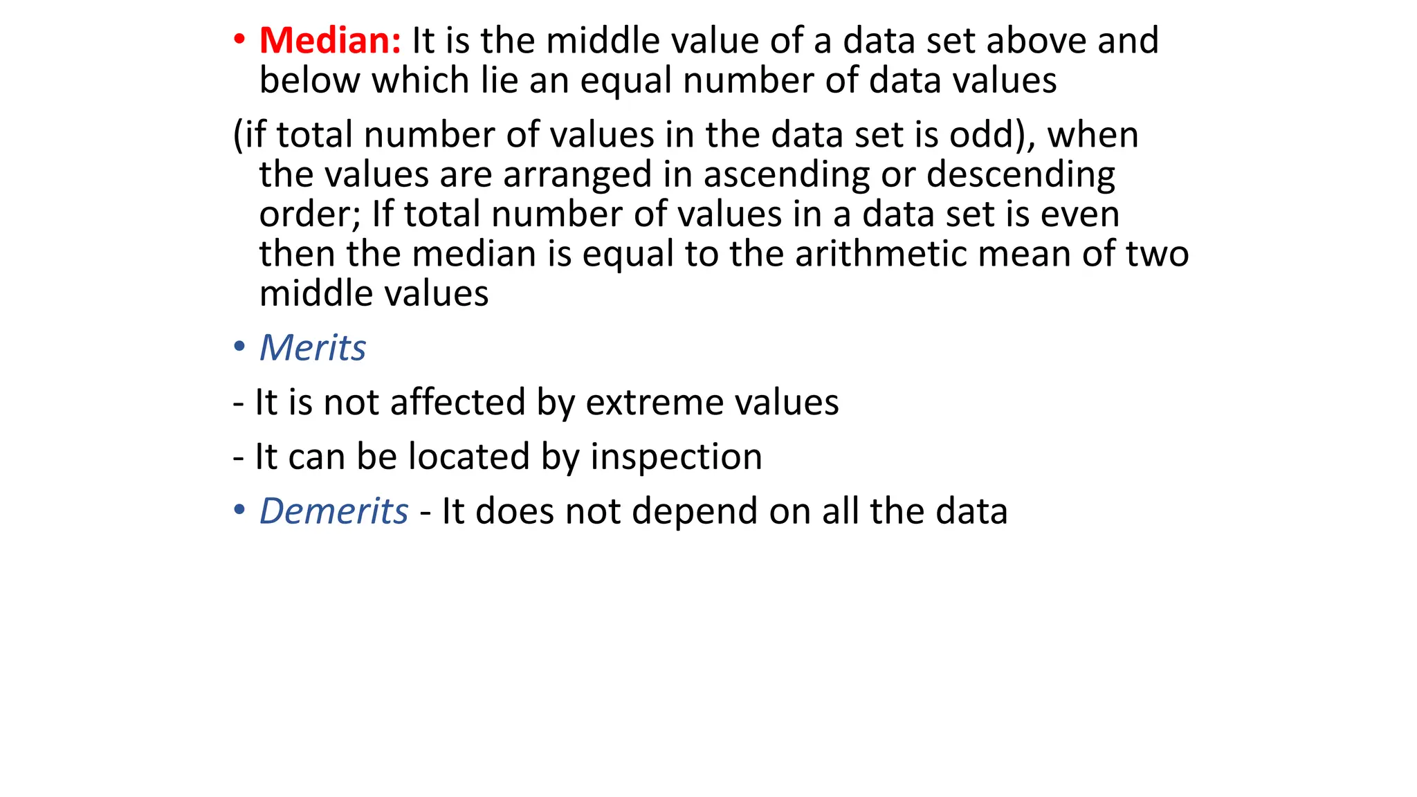
6. • Median: It is the middle value of a data set above and
below which lie an equal number of data values
(if total number of values in the data set is odd), when
the values are arranged in ascending or descending
order; If total number of values in a data set is even
then the median is equal to the arithmetic mean of two
middle values
• Merits
- It is not affected by extreme values
- It can be located by inspection
• Demerits - It does not depend on all the data

7. • Mode: It is the most frequently occurring value of a
data set
• Its merits and demerits are similar to that of median
• In addition, it can be used for qualitative data

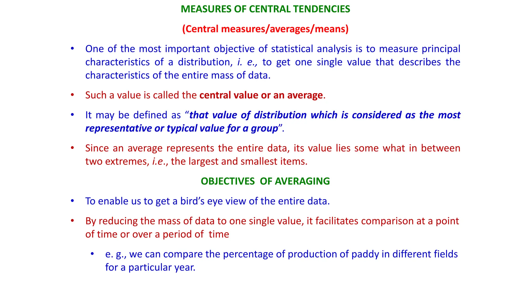
8. MEASURES OF CENTRAL TENDENCIES
(Central measures/averages/means)
• One of the most important objective of statistical analysis is to measure principal
characteristics of a distribution, i. e., to get one single value that describes the
characteristics of the entire mass of data.
• Such a value is called the central value or an average.
• It may be defined as “that value of distribution which is considered as the most
representative or typical value for a group”.
• Since an average represents the entire data, its value lies some what in between
two extremes, i.e., the largest and smallest items.
OBJECTIVES OF AVERAGING
• To enable us to get a bird’s eye view of the entire data.
• By reducing the mass of data to one single value, it facilitates comparison at a point
of time or over a period of time
• e. g., we can compare the percentage of production of paddy in different fields
for a particular year.

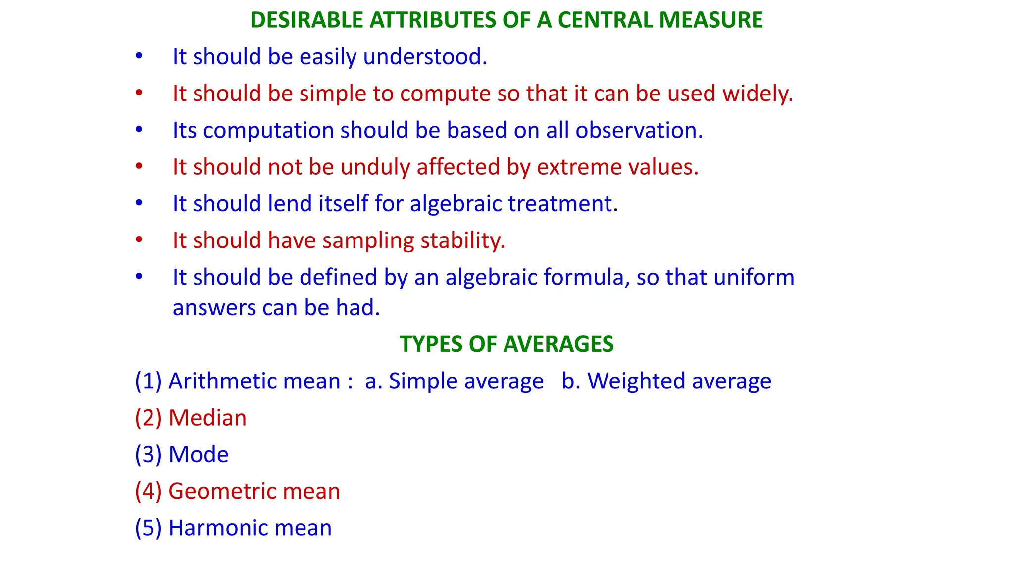
9. DESIRABLE ATTRIBUTES OF A CENTRAL MEASURE
• It should be easily understood.
• It should be simple to compute so that it can be used widely.
• Its computation should be based on all observation.
• It should not be unduly affected by extreme values.
• It should lend itself for algebraic treatment.
• It should have sampling stability.
• It should be defined by an algebraic formula, so that uniform
answers can be had.
TYPES OF AVERAGES
(1) Arithmetic mean : a. Simple average b. Weighted average
(2) Median
(3) Mode
(4) Geometric mean
(5) Harmonic mean

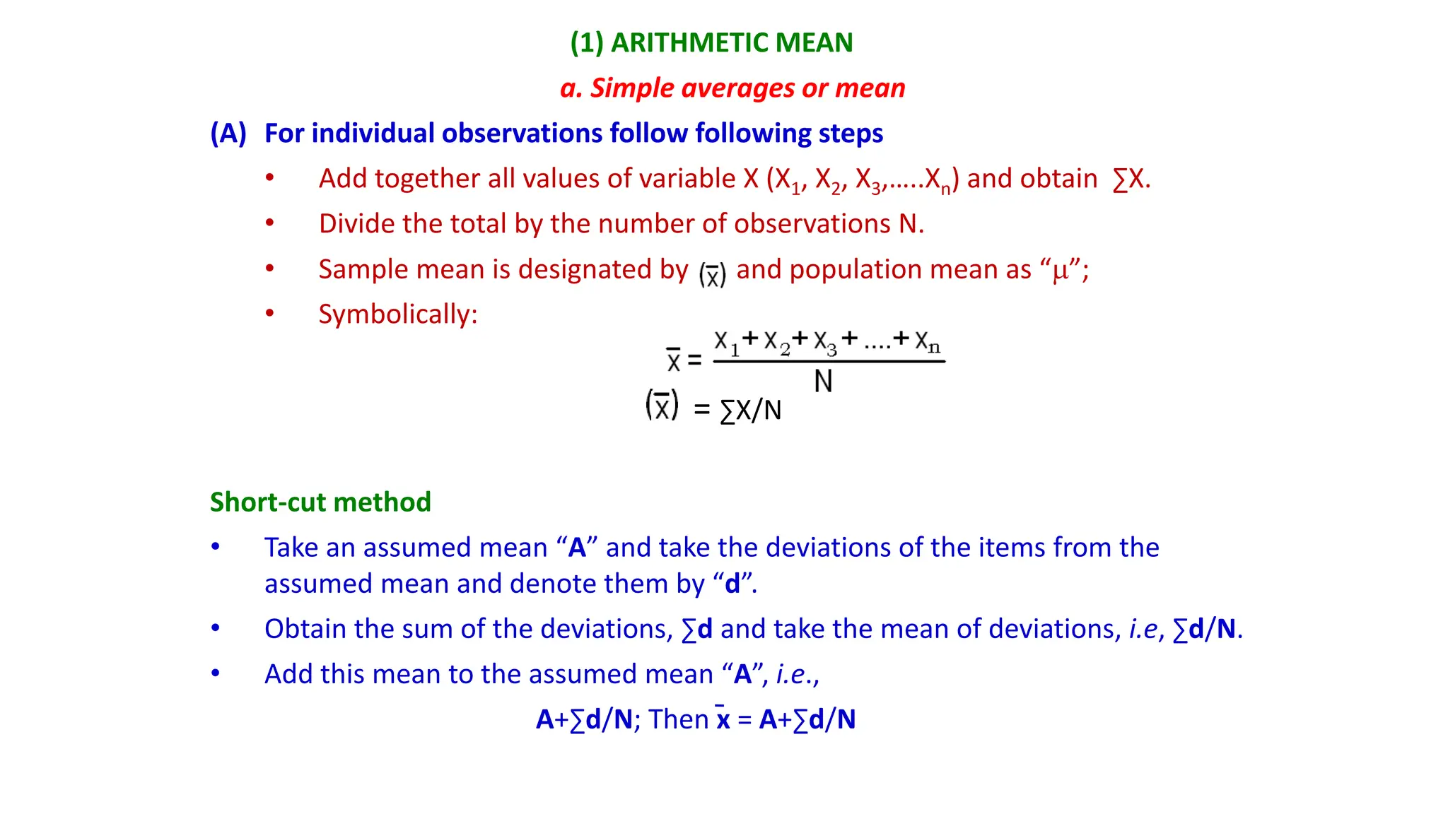
10. (1) ARITHMETIC MEAN
a. Simple averages or mean
(A) For individual observations follow following steps
• Add together all values of variable X (X1, X2, X3,…..Xn) and obtain ∑X.
• Divide the total by the number of observations N.
• Sample mean is designated by and population mean as “”;
• Symbolically:
= ∑X/N
Short-cut method
• Take an assumed mean “A” and take the deviations of the items from the
assumed mean and denote them by “d”.
• Obtain the sum of the deviations, ∑d and take the mean of deviations, i.e, ∑d/N.
• Add this mean to the assumed mean “A”, i.e.,
A+∑d/N; Then x = A+∑d/N

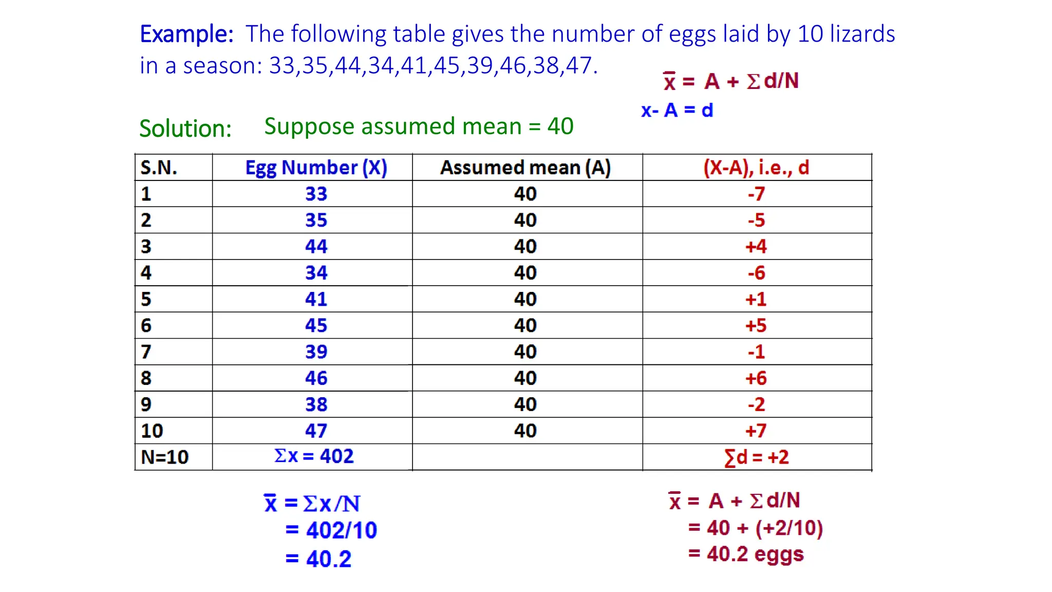
11. Example: The following table gives the number of eggs laid by 10 lizards
in a season: 33,35,44,34,41,45,39,46,38,47.
Solution: Suppose assumed mean = 40

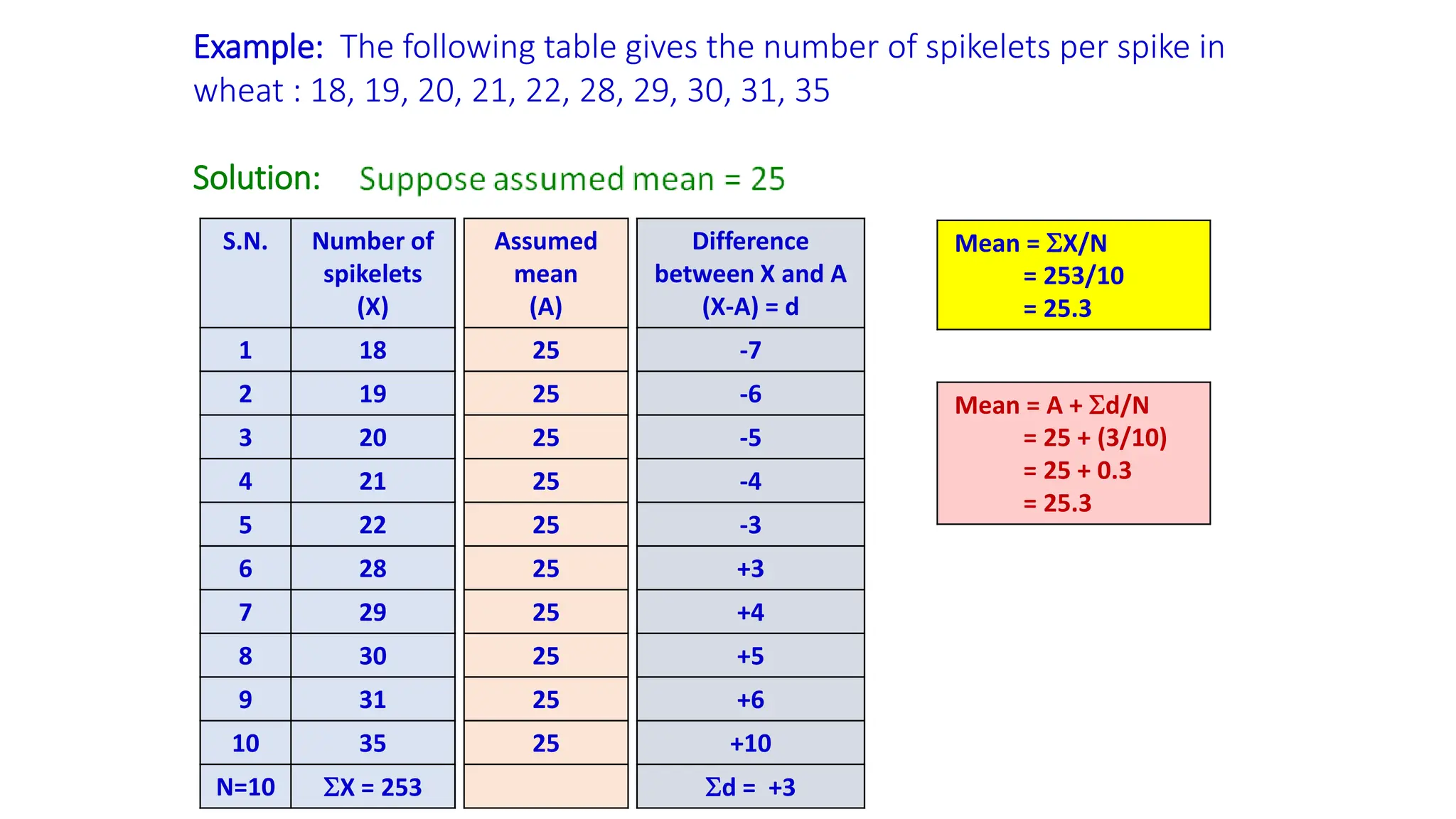
12. Example: The following table gives the number of spikelets per spike in
wheat : 18, 19, 20, 21, 22, 28, 29, 30, 31, 35
Solution:
S.N. Number of
spikelets
(X)
1 18
2 19
3 20
4 21
5 22
6 28
7 29
8 30
9 31
10 35
N=10 X = 253
Assumed
mean
(A)
25
25
25
25
25
25
25
25
25
25
Difference
between X and A
(X-A) = d
-7
-6
-5
-4
-3
+3
+4
+5
+6
+10
d = +3
Mean = X/N
= 253/10
= 25.3
Mean = A + d/N
= 25 + (3/10)
= 25 + 0.3
= 25.3

13. Weight (g) (X) No. of fishes (f)
20 8
30 12
40 20
50 10
60 6
70 4
Total ∑f or N=60
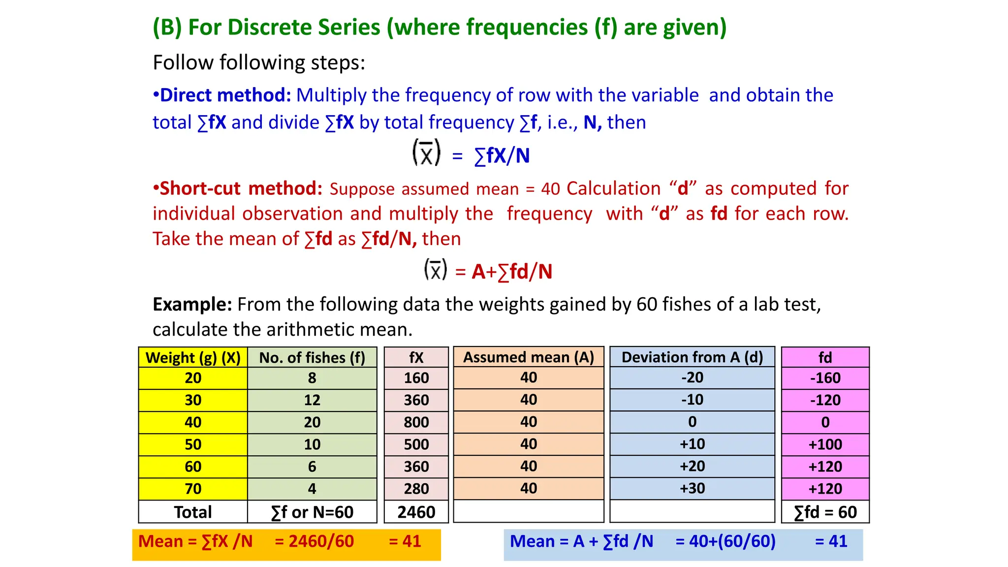
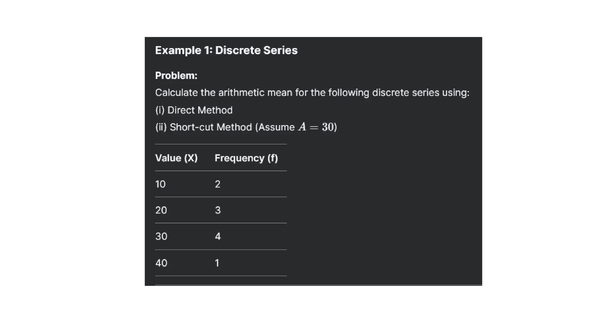
(B) For Discrete Series (where frequencies (f) are given)
Follow following steps:
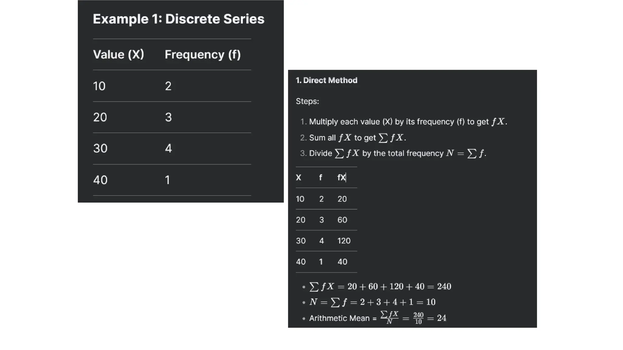
•Direct method: Multiply the frequency of row with the variable and obtain the
total ∑fX and divide ∑fX by total frequency ∑f, i.e., N, then
= ∑fX/N
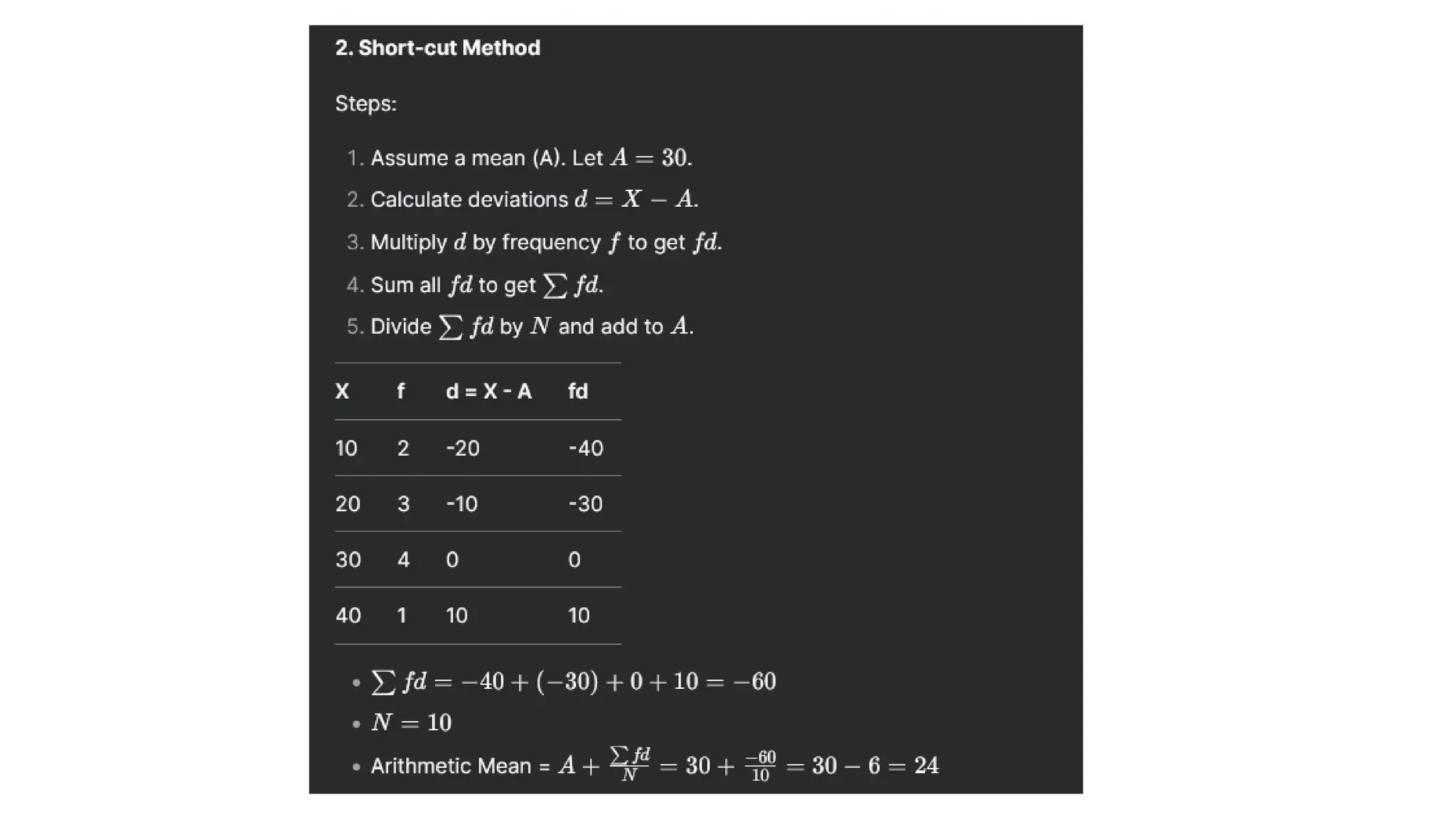
•Short-cut method: Suppose assumed mean = 40 Calculation “d” as computed for
individual observation and multiply the frequency with “d” as fd for each row.
Take the mean of ∑fd as ∑fd/N, then
= A+∑fd/N
Example: From the following data the weights gained by 60 fishes of a lab test,
calculate the arithmetic mean.
fX
160
360
800
500
360
280
2460
Assumed mean (A)
40
40
40
40
40
40
Deviation from A (d)
-20
-10
0
+10
+20
+30
fd
-160
-120
0
+100
+120
+120
∑fd = 60
Mean = ∑fX /N = 2460/60 = 41 Mean = A + ∑fd /N = 40+(60/60) = 41

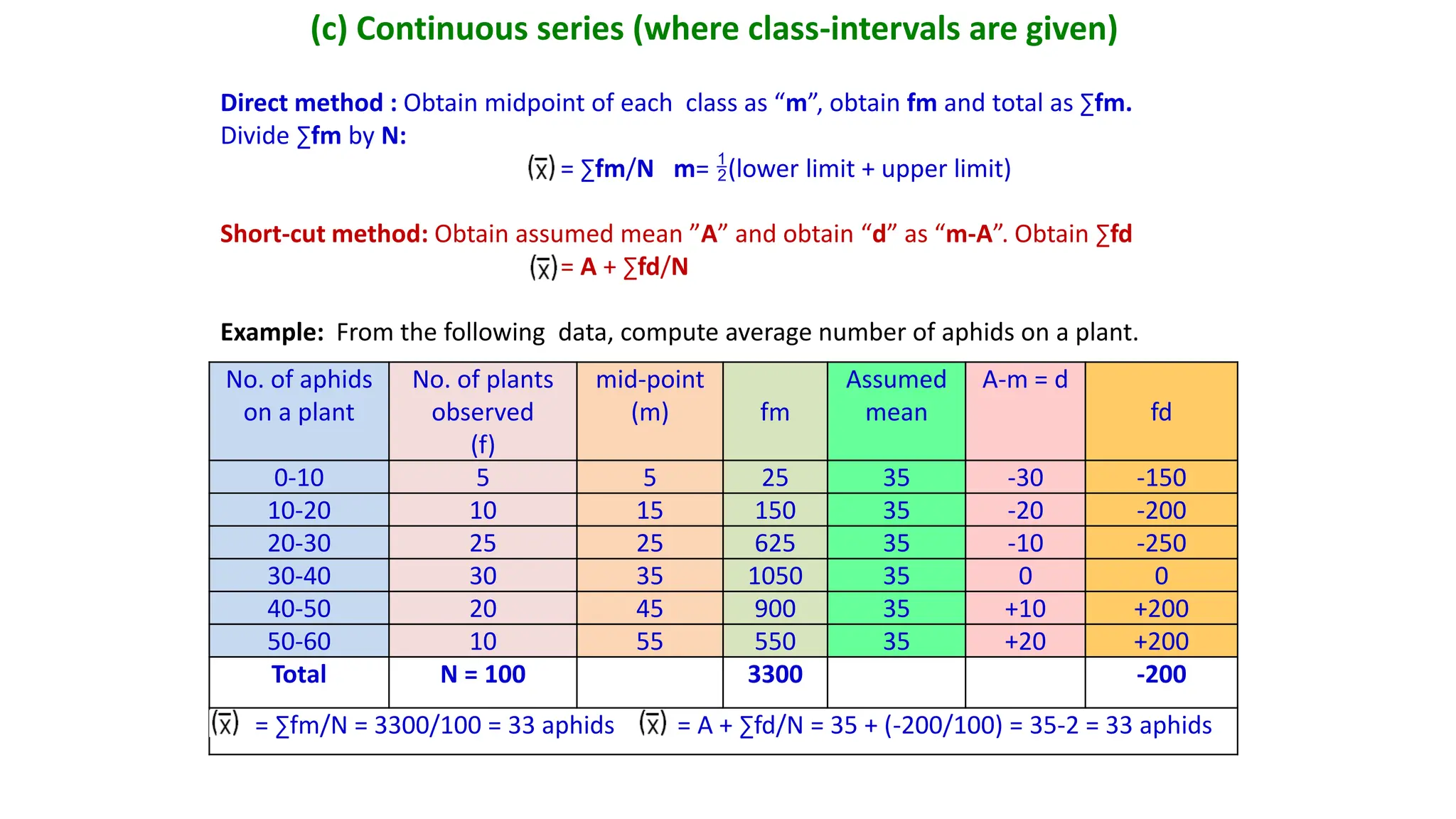
17. (c) Continuous series (where class-intervals are given)
Direct method : Obtain midpoint of each class as “m”, obtain fm and total as ∑fm.
Divide ∑fm by N:
= ∑fm/N m= (lower limit + upper limit)
Short-cut method: Obtain assumed mean ”A” and obtain “d” as “m-A”. Obtain ∑fd
= A + ∑fd/N
Example: From the following data, compute average number of aphids on a plant.
No. of aphids
on a plant
No. of plants
observed
(f)
mid-point
(m) fm
Assumed
mean
A-m = d
fd
0-10 5 5 25 35 -30 -150
10-20 10 15 150 35 -20 -200
20-30 25 25 625 35 -10 -250
30-40 30 35 1050 35 0 0
40-50 20 45 900 35 +10 +200
50-60 10 55 550 35 +20 +200
Total N = 100 3300 -200
= ∑fm/N = 3300/100 = 33 aphids = A + ∑fd/N = 35 + (-200/100) = 35-2 = 33 aphids

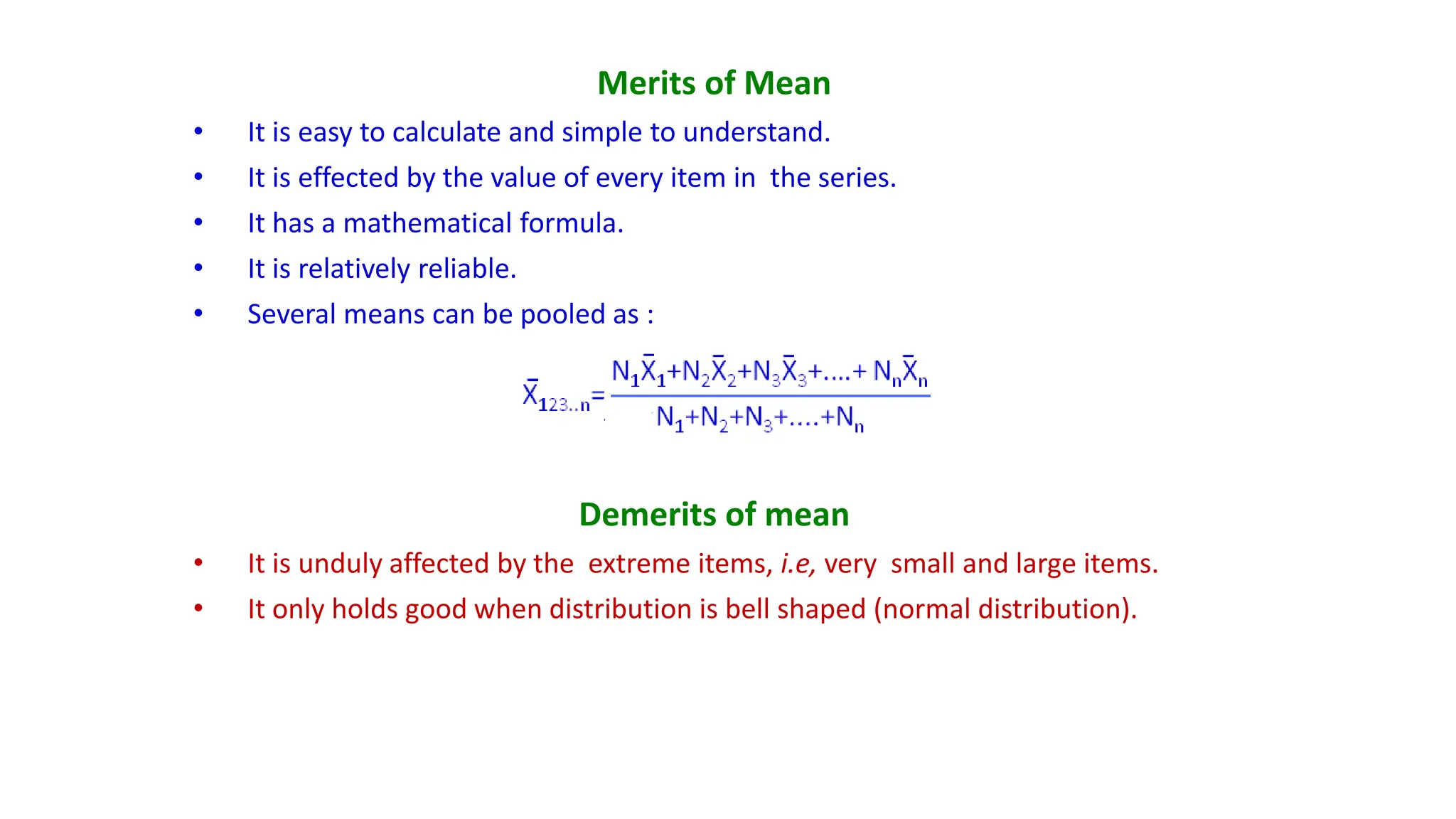
21. Merits of Mean
• It is easy to calculate and simple to understand.
• It is effected by the value of every item in the series.
• It has a mathematical formula.
• It is relatively reliable.
• Several means can be pooled as :
Demerits of mean
• It is unduly affected by the extreme items, i.e, very small and large items.
• It only holds good when distribution is bell shaped (normal distribution).

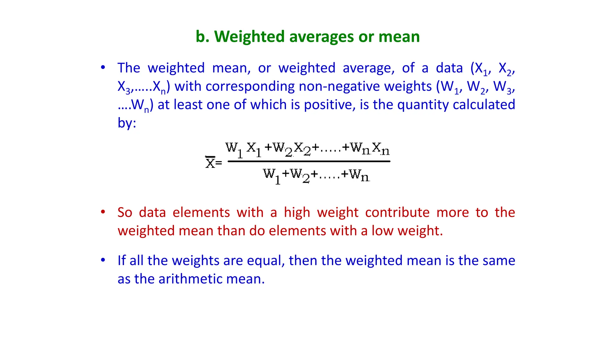
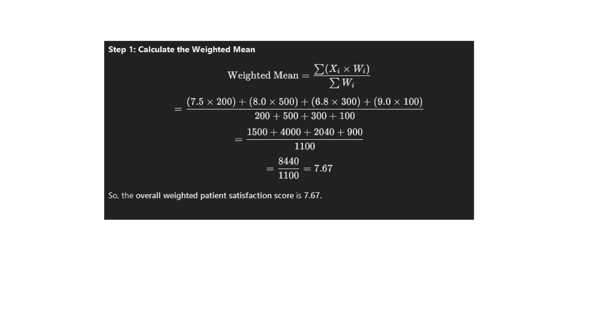
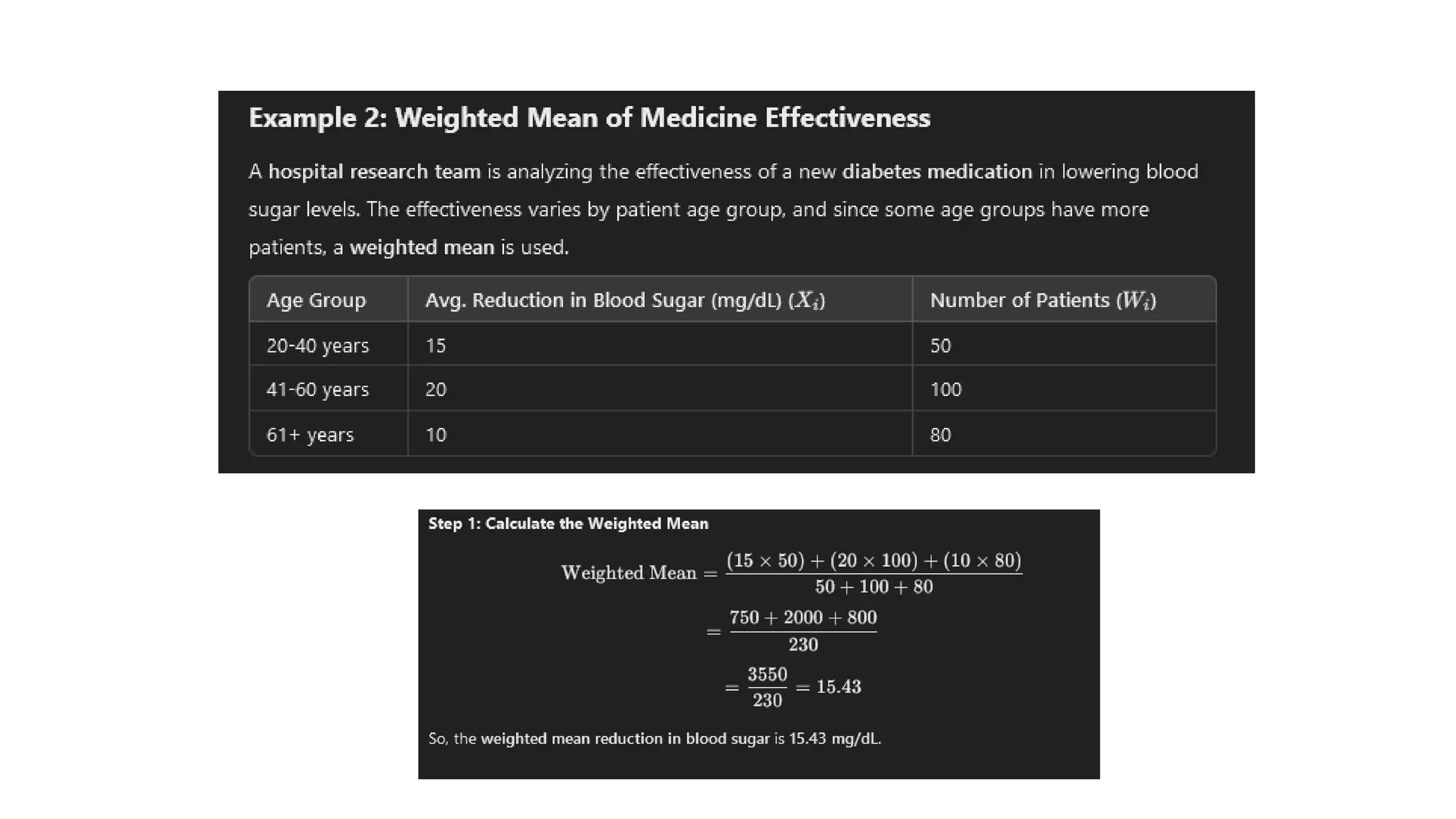
22. b. Weighted averages or mean
• The weighted mean, or weighted average, of a data (X1, X2,
X3,…..Xn) with corresponding non-negative weights (W1, W2, W3,
….Wn) at least one of which is positive, is the quantity calculated
by:
• So data elements with a high weight contribute more to the
weighted mean than do elements with a low weight.
• If all the weights are equal, then the weighted mean is the same
as the arithmetic mean.

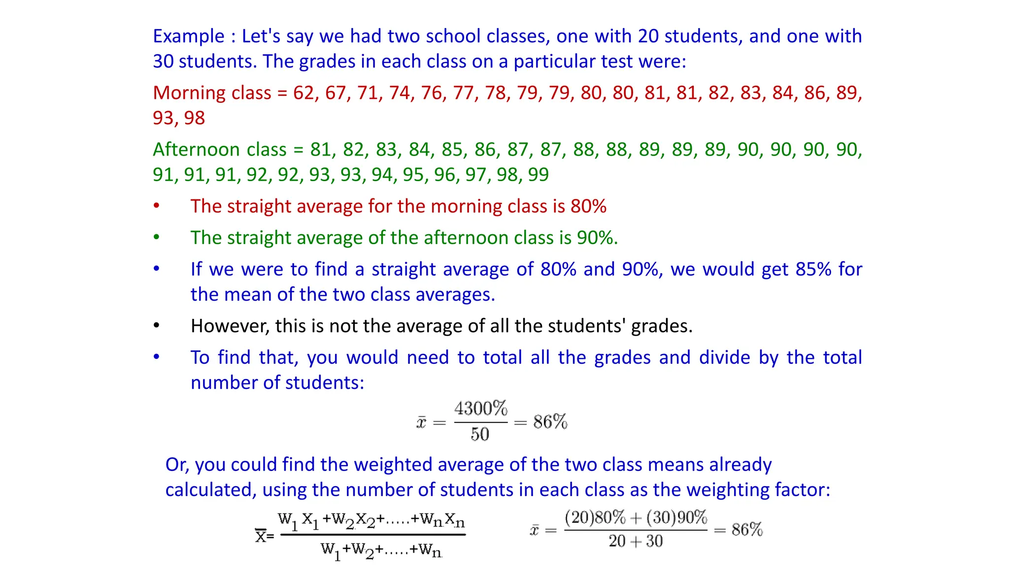
23. Example : Let's say we had two school classes, one with 20 students, and one with
30 students. The grades in each class on a particular test were:
Morning class = 62, 67, 71, 74, 76, 77, 78, 79, 79, 80, 80, 81, 81, 82, 83, 84, 86, 89,
93, 98
Afternoon class = 81, 82, 83, 84, 85, 86, 87, 87, 88, 88, 89, 89, 89, 90, 90, 90, 90,
91, 91, 91, 92, 92, 93, 93, 94, 95, 96, 97, 98, 99
• The straight average for the morning class is 80%
• The straight average of the afternoon class is 90%.
• If we were to find a straight average of 80% and 90%, we would get 85% for
the mean of the two class averages.
• However, this is not the average of all the students' grades.
• To find that, you would need to total all the grades and divide by the total
number of students:
Or, you could find the weighted average of the two class means already
calculated, using the number of students in each class as the weighting factor: