1
DEEP LEARNING JP
[DLPapers]
http://deeplearning.jp/
Matrix Capsules with EM Routing (ICLR2018)
Kazuki Fujikawa, DeNA
2.
サマリ
• 書誌情報
– ICLR2018
– Geoffrey Hinton, Sara Sabour, Nicholas Frosst
• 概要
– Dynamic Routing Between Capsules [Sabour+, NIPS2017] の続報
– カプセル層を多層化
– Poseを2Dベクトルではなく3D行列で表現
– 存在確率をベクトルのノルムではなく専用のユニットで表現
– ルーティングに混合ガウスモデルのEMアルゴリズムを用いる
– smallNORBデータセットでSOTA
2
Published asaconference paper at ICLR 2018
Figure 1: A network with one ReLU convolutional layer followed by a primary convolutional cap-
sule layer and two moreconvolutional capsule layers.
関連研究
• Dynamic RoutingBetween Capsules [Sabour+, NIPS2017]
– アーキテクチャ
22
図引用: https://medium.com/@mike_ross/a-visual-representation-of-capsule-network-computations-83767d79e737
分類誤差(margin loss)以外に、
正解クラスのcapsuleの情報のみをinputに、
再構成させ、ピクセル単位での再構成誤差
も学習に利用
→ 再構成に必要な属性(太さ、スケール etc.)
がカプセルで表現されるようになる
Figure 2: Decoder structure to reconstruct a digit from the DigitCaps layer representation. The
euclidean distance between the image and the output of the Sigmoid layer is minimized during
training. Weuse thetruelabel asreconstruction target during training.
fieldsoverlap with thelocation of thecenter of thecapsule. In total PrimaryCapsules has[32⇥6⇥6]
capsule outputs (each output is an 8D vector) and each capsule in the [6 ⇥ 6] grid is sharing their
weights with each other. One can seePrimaryCapsules asaConvolution layer with Eq. 1 asitsblock
non-linearity. The final Layer (DigitCaps) has one 16D capsule per digit class and each of these
capsules receivesinput from all thecapsules in the layer below.
Wehaverouting only between two consecutivecapsule layers (e.g. PrimaryCapsules and DigitCaps).
SinceConv1 output is1D, thereisno orientation in itsspaceto agreeon. Therefore, no routing isused
between Conv1 and PrimaryCapsules. All therouting logits (bi j ) are initialized to zero. Therefore,
initially acapsule output (ui ) issent to all parent capsules (v0...v9) with equal probability (ci j ).
Our implementation isin TensorFlow (Abadi et al. [2016]) and weusetheAdam optimizer (Kingma
and Ba[2014]) with itsTensorFlow default parameters, including theexponentially decaying learning
rate, to minimize thesum of the margin losses in Eq. 4.
4.1 Reconstruction asa regularization method
Weusean additional reconstruction lossto encourage thedigit capsules to encodetheinstantiation
parameters of theinput digit. During training, wemask out all but theactivity vector of thecorrect
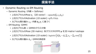
提案手法
• Matrix Capsuleswith EM Routing
– カプセル層を多層化
– Poseを2Dベクトルではなく3D行列で表現
– 存在確率をベクトルのノルムではなく専用のユニットで表現
– ルーティングに混合ガウスモデル(GMM)のEMアルゴリズムを用いる
24
Published asaconference paper at ICLR 2018
Figure 1: A network with one ReLU convolutional layer followed by a primary convolutional cap-
sule layer and two moreconvolutional capsule layers.
that location. Theactivationsof theprimary capsulesareproduced by applying thesigmoid function
to the weighted sumsof the same set of lower-layer ReLUs.
The primary capsules are followed by two 3x3 convolutional capsule layers (K=3), each with 32
capsule types (C=D=32) with strides of 2 and one, respectively. The last layer of convolutional
提案手法
• Margin loss[Sabour+, NIPS2017]
• Spread loss [Hinton+, ICLR2018]
– ベースはMargin loss
– 正解となるクラスのスコアが、不正解となるクラスのスコアよりも大きくなるように
するということを明示的に定式化
• Coordinate addition
– 最終層では、全カプセルがクラスカプセルへ結合し、元のxy座標の情報を失う
– アフィン変換先の特徴空間でも同じような位置関係になるように、xy座標をスケーリング
したものを、各クラスカプセルの最初の2成分へ足し込む
34
SS
he training less sensitive to the initialization and hyper-parameters of the model,
s” to directly maximize thegap between theactivation of thetarget class(at ) and
e other classes. If the activation of a wrong class, ai , is closer than the margin,
enalized by thesquared distance to themargin:
Li = (max(0, m − (at − ai ))2
, L =
X
i 6= t
Li (3)
small margin of 0.2 and linearly increasing it during training to 0.9, we avoid
he earlier layers. Spread loss is equivalent to squared Hinge loss with m = 1.
rini (2011) studies avariant of thislossin thecontext of multi class SVMs.
NTS
ataset (LeCun et al. (2004)) has gray-level stereo images of 5 classes of toys:
ks, humansand animals. Thereare10 physical instances of each classwhich are
n. 5 physical instances of aclass areselected for thetraining dataand theother 5
very individual toy is pictured at 18 different azimuths (0-340), 9 elevations and
ns, so thetraining and test setseach contain 24,300 stereo pairsof 96x96 images.
NORB asabenchmark for developing our capsules system because it iscarefully
実験
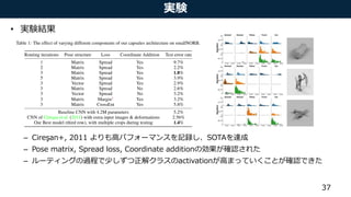
• 実験結果
– Cireşan+,2011 よりも高パフォーマンスを記録し、SOTAを達成
– Pose matrix, Spread loss, Coordinate additionの効果が確認された
– ルーティングの過程で少しずつ正解クラスのactivationが高まっていくことが確認できた
37
Figure 2: Histogram of distances of votes to the mean of each of the 5 final capsules after each
routing iteration. Each distance point is weighted by its assignment probability. All three images
are selected from the smallNORB test set. The routing procedure correctly routes the votes in the
truck and the human example. The plane example shows a rare failure case of the model where the
planeisconfused with acar in thethird routing iteration. Thehistograms arezoomed-in to visualize
only votes with distances less than 0.05. Fig. B.2 shows the complete histograms for the ”human”
capsule without clipping the x-axis or fixing thescale of the y-axis.
38.
References
• Hinton, G.,Frosst, N., & Sabour, S. (2018). Matrix capsules with EM routing. Hinton, G.,
Frosst, N., & Sabour, S. (2018). Matrix capsules with EM routing. ICLR2018.
• Sabour, S., Frosst, N., & Hinton, G. E. (2017). Dynamic routing between capsules.
In Advances in Neural Information Processing Systems (pp. 3859-3869).
• Cireşan, Dan C., et al. "High-performance neural networks for visual object
classification." arXiv preprint arXiv:1102.0183 (2011).
38
![1
DEEP LEARNING JP
[DL Papers]
http://deeplearning.jp/
Matrix Capsules with EM Routing (ICLR2018)
Kazuki Fujikawa, DeNA](https://image.slidesharecdn.com/matrixcapsuleswithemrouting-180423120251/85/Matrix-capsules-with-em-routing-1-320.jpg)
![サマリ
• 書誌情報
– ICLR 2018
– Geoffrey Hinton, Sara Sabour, Nicholas Frosst
• 概要
– Dynamic Routing Between Capsules [Sabour+, NIPS2017] の続報
– カプセル層を多層化
– Poseを2Dベクトルではなく3D行列で表現
– 存在確率をベクトルのノルムではなく専用のユニットで表現
– ルーティングに混合ガウスモデルのEMアルゴリズムを用いる
– smallNORBデータセットでSOTA
2
Published asaconference paper at ICLR 2018
Figure 1: A network with one ReLU convolutional layer followed by a primary convolutional cap-
sule layer and two moreconvolutional capsule layers.](https://image.slidesharecdn.com/matrixcapsuleswithemrouting-180423120251/85/Matrix-capsules-with-em-routing-2-320.jpg)


![関連研究
• Dynamic Routing Between Capsules [Sabour+, NIPS2017]
– 特徴をスカラーではなくベクトルで表す
• 特徴量(スカラー): 着目した特徴の存在有無を表す
– 同じオブジェクトで異なる姿勢の特徴は別ユニットで表現せざるを得ない
• 特徴量(ベクトル): 着目した特徴に関して、姿勢などの任意の属性を表現可能
– 同じオブジェクトで異なる姿勢の特徴を同一のカプセルで表現することが原理的には可能
– カプセル: ユニットの集合
8図引用: https://medium.com/ai%C2%B3-theory-practice-business/understanding-hintons-capsule-networks-part-ii-how-capsules-work-153b6ade9f66](https://image.slidesharecdn.com/matrixcapsuleswithemrouting-180423120251/85/Matrix-capsules-with-em-routing-8-320.jpg)
![関連研究
• Dynamic Routing Between Capsules [Sabour+, NIPS2017]
– アーキテクチャ
9
図引用: https://medium.com/@mike_ross/a-visual-representation-of-capsule-network-computations-83767d79e737](https://image.slidesharecdn.com/matrixcapsuleswithemrouting-180423120251/85/Matrix-capsules-with-em-routing-9-320.jpg)
![関連研究
• Dynamic Routing Between Capsules [Sabour+, NIPS2017]
– アーキテクチャ
10
図引用: https://medium.com/@mike_ross/a-visual-representation-of-capsule-network-computations-83767d79e737
画像から普通のCNNで特徴抽出、
6x6, 256チャンネルの
feature mapを獲得](https://image.slidesharecdn.com/matrixcapsuleswithemrouting-180423120251/85/Matrix-capsules-with-em-routing-10-320.jpg)
![関連研究
• Dynamic Routing Between Capsules [Sabour+, NIPS2017]
– アーキテクチャ
11
図引用: https://medium.com/@mike_ross/a-visual-representation-of-capsule-network-computations-83767d79e737
256チャンネルのfeature mapを
8チャンネル区切りにreshapeし、
8Dベクトルが 6x6, 32チャンネル
あると考える](https://image.slidesharecdn.com/matrixcapsuleswithemrouting-180423120251/85/Matrix-capsules-with-em-routing-11-320.jpg)
![関連研究
• Dynamic Routing Between Capsules [Sabour+, NIPS2017]
– アーキテクチャ
12
図引用: https://medium.com/@mike_ross/a-visual-representation-of-capsule-network-computations-83767d79e737
Squashする
Squash: ベクトルの方向を維持しながら
ノルムが0~1になるようにスケーリング
引用: https://jhui.github.io/2017/11/03/Dynamic-Routing-
Between-Capsules/](https://image.slidesharecdn.com/matrixcapsuleswithemrouting-180423120251/85/Matrix-capsules-with-em-routing-12-320.jpg)
![関連研究
• Dynamic Routing Between Capsules [Sabour+, NIPS2017]
– アーキテクチャ
13
図引用: https://medium.com/@mike_ross/a-visual-representation-of-capsule-network-computations-83767d79e737
Flattenする](https://image.slidesharecdn.com/matrixcapsuleswithemrouting-180423120251/85/Matrix-capsules-with-em-routing-13-320.jpg)
![関連研究
• Dynamic Routing Between Capsules [Sabour+, NIPS2017]
– アーキテクチャ
14
図引用: https://medium.com/@mike_ross/a-visual-representation-of-capsule-network-computations-83767d79e737
各ベクトル(カプセル)は
特定の特徴を表し、そのノルムが
存在有無を表している](https://image.slidesharecdn.com/matrixcapsuleswithemrouting-180423120251/85/Matrix-capsules-with-em-routing-14-320.jpg)
![関連研究
• Dynamic Routing Between Capsules [Sabour+, NIPS2017]
– アーキテクチャ
15
図引用: https://medium.com/@mike_ross/a-visual-representation-of-capsule-network-computations-83767d79e737
各カプセルは、自身の情報𝑢𝑖を手がかりに、クラス毎に
異なる重み𝐖𝑖𝑗でアフィン変換して各クラスの特徴 (pose)
を予測する
𝐮𝑗|𝑖 = 𝐖𝑖𝑗 𝐮𝑖](https://image.slidesharecdn.com/matrixcapsuleswithemrouting-180423120251/85/Matrix-capsules-with-em-routing-15-320.jpg)
![関連研究
• Dynamic Routing Between Capsules [Sabour+, NIPS2017]
– アーキテクチャ
16
図引用: https://medium.com/@mike_ross/a-visual-representation-of-capsule-network-computations-83767d79e737
各下位カプセルが予測した上位カプセル 𝐮𝑗|𝑖を、
𝑐𝑖𝑗で重み付けして和をとり、squash
して出力カプセル𝐯𝑗を得る
( 𝑐𝑖𝑗 をDynamic Routingで計算する)
𝐯𝑗 = 𝑠𝑞𝑢𝑎𝑠ℎ(
𝑖
𝑐𝑖𝑗 𝑢𝑗|𝑖)](https://image.slidesharecdn.com/matrixcapsuleswithemrouting-180423120251/85/Matrix-capsules-with-em-routing-16-320.jpg)
![関連研究
• Dynamic Routing Between Capsules [Sabour+, NIPS2017]
– アーキテクチャ
17
図引用: https://medium.com/@mike_ross/a-visual-representation-of-capsule-network-computations-83767d79e737
𝑏𝑖𝑗: 下位カプセルiと上位カプセルj
の関連度(になっていく)
最初はゼロ埋め](https://image.slidesharecdn.com/matrixcapsuleswithemrouting-180423120251/85/Matrix-capsules-with-em-routing-17-320.jpg)
![関連研究
• Dynamic Routing Between Capsules [Sabour+, NIPS2017]
– アーキテクチャ
18
図引用: https://medium.com/@mike_ross/a-visual-representation-of-capsule-network-computations-83767d79e737
𝐛𝑖をjに関してsoftmax
下位カプセルiの割当先を
どれか一つに絞る
(最初は均等)](https://image.slidesharecdn.com/matrixcapsuleswithemrouting-180423120251/85/Matrix-capsules-with-em-routing-18-320.jpg)
![関連研究
• Dynamic Routing Between Capsules [Sabour+, NIPS2017]
– アーキテクチャ
19
図引用: https://medium.com/@mike_ross/a-visual-representation-of-capsule-network-computations-83767d79e737
予測出力カプセル 𝐮𝑗|𝑖を𝑐𝑖𝑗で
重み付けし、iに関して
足し合わせる](https://image.slidesharecdn.com/matrixcapsuleswithemrouting-180423120251/85/Matrix-capsules-with-em-routing-19-320.jpg)
![関連研究
• Dynamic Routing Between Capsules [Sabour+, NIPS2017]
– アーキテクチャ
20
図引用: https://medium.com/@mike_ross/a-visual-representation-of-capsule-network-computations-83767d79e737
Squashしてノルムが0~1になる
ようにスケーリングし、
各クラスの予測カプセルとする](https://image.slidesharecdn.com/matrixcapsuleswithemrouting-180423120251/85/Matrix-capsules-with-em-routing-20-320.jpg)
![関連研究
• Dynamic Routing Between Capsules [Sabour+, NIPS2017]
– アーキテクチャ
21
図引用: https://medium.com/@mike_ross/a-visual-representation-of-capsule-network-computations-83767d79e737
𝑏𝑖𝑗を 𝐮𝑗|𝑖と𝐯𝑗の内積を足すことで更新
𝐮𝑗|𝑖と𝐯𝑗の関連が強い要素が大きくなる](https://image.slidesharecdn.com/matrixcapsuleswithemrouting-180423120251/85/Matrix-capsules-with-em-routing-21-320.jpg)
![関連研究
• Dynamic Routing Between Capsules [Sabour+, NIPS2017]
– アーキテクチャ
22
図引用: https://medium.com/@mike_ross/a-visual-representation-of-capsule-network-computations-83767d79e737
分類誤差(margin loss)以外に、
正解クラスのcapsuleの情報のみをinputに、
再構成させ、ピクセル単位での再構成誤差
も学習に利用
→ 再構成に必要な属性(太さ、スケール etc.)
がカプセルで表現されるようになる
Figure 2: Decoder structure to reconstruct a digit from the DigitCaps layer representation. The
euclidean distance between the image and the output of the Sigmoid layer is minimized during
training. Weuse thetruelabel asreconstruction target during training.
fieldsoverlap with thelocation of thecenter of thecapsule. In total PrimaryCapsules has[32⇥6⇥6]
capsule outputs (each output is an 8D vector) and each capsule in the [6 ⇥ 6] grid is sharing their
weights with each other. One can seePrimaryCapsules asaConvolution layer with Eq. 1 asitsblock
non-linearity. The final Layer (DigitCaps) has one 16D capsule per digit class and each of these
capsules receivesinput from all thecapsules in the layer below.
Wehaverouting only between two consecutivecapsule layers (e.g. PrimaryCapsules and DigitCaps).
SinceConv1 output is1D, thereisno orientation in itsspaceto agreeon. Therefore, no routing isused
between Conv1 and PrimaryCapsules. All therouting logits (bi j ) are initialized to zero. Therefore,
initially acapsule output (ui ) issent to all parent capsules (v0...v9) with equal probability (ci j ).
Our implementation isin TensorFlow (Abadi et al. [2016]) and weusetheAdam optimizer (Kingma
and Ba[2014]) with itsTensorFlow default parameters, including theexponentially decaying learning
rate, to minimize thesum of the margin losses in Eq. 4.
4.1 Reconstruction asa regularization method
Weusean additional reconstruction lossto encourage thedigit capsules to encodetheinstantiation
parameters of theinput digit. During training, wemask out all but theactivity vector of thecorrect](https://image.slidesharecdn.com/matrixcapsuleswithemrouting-180423120251/85/Matrix-capsules-with-em-routing-22-320.jpg)


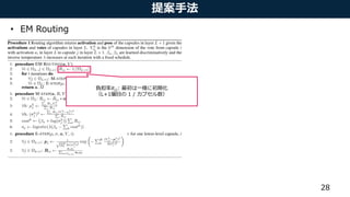
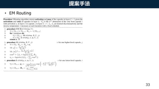
![提案手法
• EM Routing
27
[Sabour+, NIPS2017]
• Input
• 𝐮𝑗|𝑖: L層目カプセルが予測するpose vector
• Output
• 𝐯𝑗: L+1層目カプセルの最終的なpose vector
[Hinton+, ICLR2018]
• Input
• 𝑉: L層目カプセルが予測するpose matrix
• 𝒂: L層目カプセル自身のactivation
• Output
• 𝑀: L+1層目カプセルの最終的なpose matrix
• 𝒂: L+1層目カプセルのactivation](https://image.slidesharecdn.com/matrixcapsuleswithemrouting-180423120251/85/Matrix-capsules-with-em-routing-27-320.jpg)


![提案手法
• Margin loss [Sabour+, NIPS2017]
• Spread loss [Hinton+, ICLR2018]
– ベースはMargin loss
– 正解となるクラスのスコアが、不正解となるクラスのスコアよりも大きくなるように
するということを明示的に定式化
• Coordinate addition
– 最終層では、全カプセルがクラスカプセルへ結合し、元のxy座標の情報を失う
– アフィン変換先の特徴空間でも同じような位置関係になるように、xy座標をスケーリング
したものを、各クラスカプセルの最初の2成分へ足し込む
34
SS
he training less sensitive to the initialization and hyper-parameters of the model,
s” to directly maximize thegap between theactivation of thetarget class(at ) and
e other classes. If the activation of a wrong class, ai , is closer than the margin,
enalized by thesquared distance to themargin:
Li = (max(0, m − (at − ai ))2
, L =
X
i 6= t
Li (3)
small margin of 0.2 and linearly increasing it during training to 0.9, we avoid
he earlier layers. Spread loss is equivalent to squared Hinge loss with m = 1.
rini (2011) studies avariant of thislossin thecontext of multi class SVMs.
NTS
ataset (LeCun et al. (2004)) has gray-level stereo images of 5 classes of toys:
ks, humansand animals. Thereare10 physical instances of each classwhich are
n. 5 physical instances of aclass areselected for thetraining dataand theother 5
very individual toy is pictured at 18 different azimuths (0-340), 9 elevations and
ns, so thetraining and test setseach contain 24,300 stereo pairsof 96x96 images.
NORB asabenchmark for developing our capsules system because it iscarefully](https://image.slidesharecdn.com/matrixcapsuleswithemrouting-180423120251/85/Matrix-capsules-with-em-routing-34-320.jpg)


![[PRML] パターン認識と機械学習(第1章:序論)](https://cdn.slidesharecdn.com/ss_thumbnails/prmlchapter1-170903070406-thumbnail.jpg?width=640&height=640&fit=bounds)


![[DL輪読会]Graph R-CNN for Scene Graph Generation](https://cdn.slidesharecdn.com/ss_thumbnails/graphr-cnnforscenegraphgenerationkobayashi1130-181130001547-thumbnail.jpg?width=640&height=640&fit=bounds)


![[DL輪読会]Xception: Deep Learning with Depthwise Separable Convolutions](https://cdn.slidesharecdn.com/ss_thumbnails/2017-06-22-170623004409-thumbnail.jpg?width=640&height=640&fit=bounds)


![[論文紹介] Convolutional Neural Network(CNN)による超解像](https://cdn.slidesharecdn.com/ss_thumbnails/cnn-presen-161218113749-thumbnail.jpg?width=640&height=640&fit=bounds)
![[DL輪読会]EfficientNet: Rethinking Model Scaling for Convolutional Neural Networks](https://cdn.slidesharecdn.com/ss_thumbnails/yokota20190621dlhack-190621022108-thumbnail.jpg?width=640&height=640&fit=bounds)


![[DL輪読会]Convolutional Conditional Neural Processesと Neural Processes Familyの紹介](https://cdn.slidesharecdn.com/ss_thumbnails/20191220readingpaperconvcnp-191220034420-thumbnail.jpg?width=640&height=640&fit=bounds)

![[DL輪読会]"Dynamical Isometry and a Mean Field Theory of CNNs: How to Train 10,0...](https://cdn.slidesharecdn.com/ss_thumbnails/wakasugi-180824003300-thumbnail.jpg?width=640&height=640&fit=bounds)