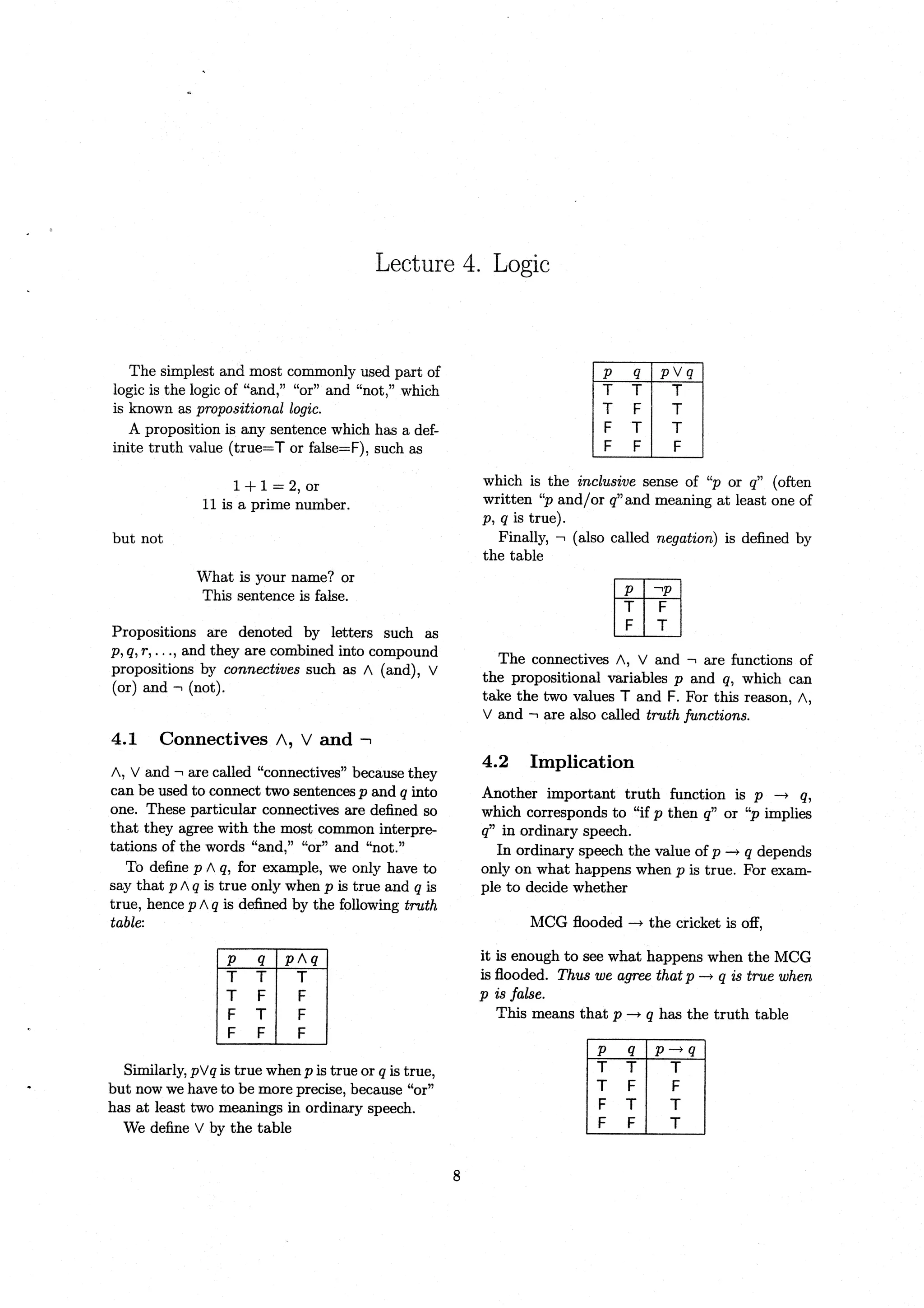
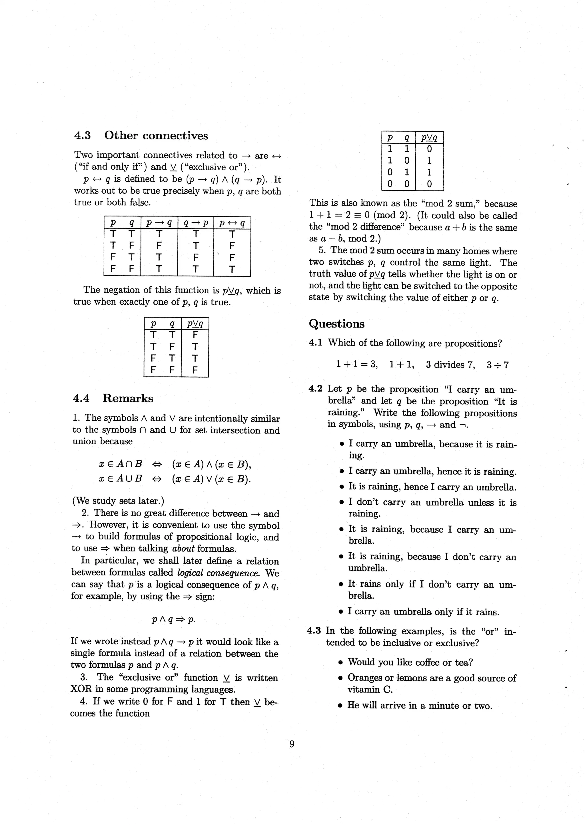
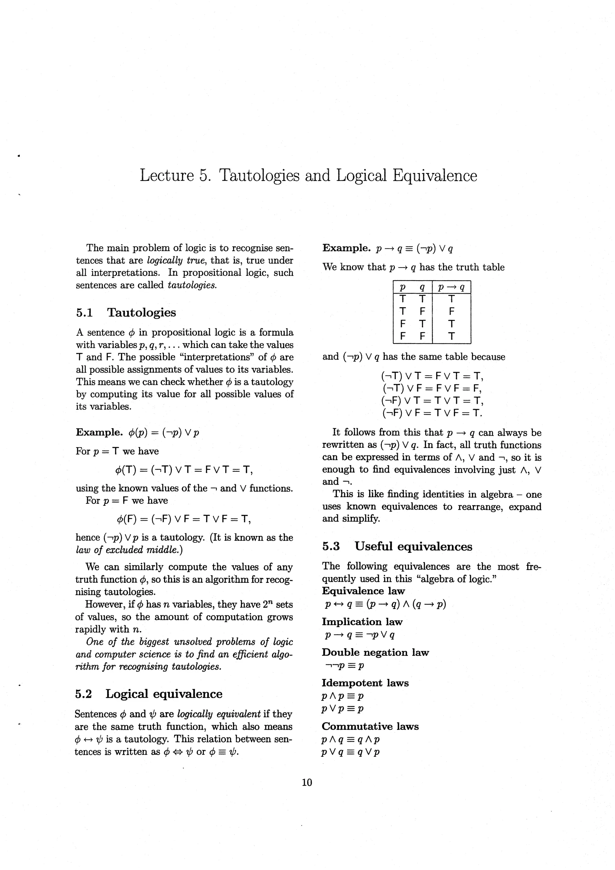
MAT1830
Discrete Mathematics for Computer Science
Lecture Notes
Prepared by John Stillwell and Daniel Delbourgo.
Edited by Chris Hough and Tom Hall.
Contents
Lecture 1: Where’s the Proof?
Lecture 2: Divisors and Primes
Lecture 3: Decimal and Other Notations
Lecture 4: Logic
Lecture 5: Tautologies and Logical Equivalence
Lecture 6: Rules of Inference
Lecture 7: Predicates and Quantifiers
Lecture 8: Predicate Logic
Lecture 9: Mathematical Induction
Lecture 10: Induction and Well-ordering
Lecture 11: Sets
Lecture 12: Operations on Sets
Lecture 13: Functions
Lecture 14: Examples of Functions
Lecture 15: Composition and Inversion
Lecture 16: Relations
Lecture 17: Equivalence Relations
Lecture 18: Order Relations
Lecture 19: Recursion
Lecture 20: Recursive Algorithms
Lecture 21: Recursion, Lists and Sequences
Lecture 22: Solving Recurrence Relations
Lecture 23: More Difficult Recurrence Relations
Lecture 24: Inhomogeneous Recurrence Relations
Lecture 25: Arithmetic and Geometric Means
Lecture 26: Graphs
Lecture 27: Walks, Paths and Trails
Lecture 28: Degree
Lecture 29: Trees
Lecture 30: Trees, Queues and Stacks
Lecture 31: Planar Graphs
Lecture 32: Congruences
Lecture 33: Random Number Generators
Lecture 34: The RSA Cryptosystem
Unit Information
MAT1830 – Semester 1 2014
Course coordinator and lecturer (Clayton)
• Name: Dr. Daniel Horsley
• Office: 28/418
• Phone: 9905 4459
• Email: daniel.horsley@monash.edu
Lecturer (Clayton)
• Name: A/Prof David Wood
• Office: 28/424
• Phone: 9905 4417
• Email: david.wood@monash.edu
Lecturer (Sunway)
• Name: Dr. Lee Kien Foo
• Email: foo.lee.kien@monash.edu
Moodle Page
The course’s Moodle page can be accessed through the my.monash portal at https://my.monash.edu.au/
Unit Guide
The full unit guide can be found at http://www.infotech.monash.edu.au/units/mat1830/ It contains a
topic outline and information on assessment, special consideration, plagiarism etc.
Course Information
• Lecture times (Clayton): Mon 3:00–4:00 in 21/S7, Wed 4:00–5:00 in 08/R4, Fri 1:00–2:00 in 25/S3.
(Lectures run in weeks 1–12.)
• Support classes: One per week as allocated. (Tutorials run in weeks 2–12.)
• Required materials: Course notes booklet - available for less than $10 from the Clayton campus
bookshop or available as a pdf from the course Moodle page. Note that there is no required textbook
for the course.
Recordings of the lectures will be available through http://www.mulo.monash.edu.au/
Assessment
• Ten assignments worth 3% each (one due each week from week 3 to week 12).
• Final examination worth 70% (held in the examination period).
In order to pass the course you must receive at least 50% overall AND at least 40% for the assignments
AND at least 40% for the exam.
The assignments will be issued in lectures and will be available from the course Moodle page. Assignments
are to be submitted to your tutor during your support class. They will then be marked and returned to you
in your next support class. No calculators or other materials will be allowed in the final exam.
Mathematics Learning Centre
The Mathematics Learning Centre is open weekdays from 11–2 in 28/G24. You can drop in for help anytime
during these hours.
Lecture 1. Where’s the proof?
1.1 What this subject is about
Discrete mathematics studies objects which
have distinct separated values (e.g. integers),
as opposed to objects which vary smoothly
(e.g. real numbers). You can think of it as
being “digital” mathematics rather than “ana-
logue” mathematics.
Discrete mathematics is particularly impor-
tant in computer science and the two fields are
very closely linked.
This course covers a wide range of topics in
discrete mathematics including the following:
• Numbers
• Logic
• Induction and recursion
• Sets, functions and relations
• Graph theory
• Cryptography
1.2 What to expect
What we do here might be a bit different to a
lot of the maths you’ve done in the past. We’ll
be concentrating on really understanding the
concepts, rather than simply learning how to
solve certain types of questions.
For a lot of the questions we ask, there won’t
be a single fixed procedure you can apply to
get the answer. Instead, you’ll have to think
carefully about what the question is asking and
try to work out what is really going on. Don’t
be afraid to try different things, play around,
and look at examples.
We’ll also be emphasising the importance of
proving results.
1.3 Proofs
A proof is essentially just a water-tight argu-
ment that a certain statement must be true.
As we’ll see, even if you are pretty sure that
something is true, it can be really useful to
have a proof of it, for a number of reasons.
1.4 Maths in computer science
As we mentioned above, maths and computer
science are very closely related. The topics in
this course all have many applications to com-
puter science. For example:
• Number theory is used in cryptography to
enable secure communication, identity veri-
fication, online banking and shopping etc.
• Logic is used in digital circuit design and in
program control flow.
• Induction and recursion are used to study
algorithms and their effectiveness.
• Functions are important in the theory of
programming and relations are vital in
database theory and design.
• Graph theory is used in software which
solves allocation and scheduling problems.
Questions
1.1 What maths that you’ve done in the past
would count as discrete? What would
count as continuous instead? Are there
grey areas?
1.2 Why might proofs be important to math-
ematicians and computer scientists?
1.3 Can you think of other links between
maths and computer science.
Lecture 3. Decimal and Other Notations
The usual notation for numbers is called
decimal or base 10 because it is based on the
number 10.
For example, 1937 stands for the number
1 × 10³
+ 9 × 10²
+ 3 × 101
+ 7.
Notice that the digits are obtained, in re-
verse order, by repeatedly dividing by 10
and discarding the remainders:
1937 divided by 10 is 193, remainder 7.
193 divided by 10 is 19, remainder 3.
19 divided by 10 is 1, remainder 9.
1 divided by 10 is 0, remainder 1.
Thus the remainders, in reverse order, are
1,9,3,7.
3.1 Base 2 notation
Exactly the same idea is used to find the
base 2 numeral for a positive integer: repeat-
edly divide by 2, discard the remainders, and
then write them down in reverse order. E.g.
1937 divided by 2 is 968, remainder 1.
968 divided by 2 is 484, remainder 0.
484 divided by 2 is 242, remainder 0.
242 divided by 2 is 121, remainder 0.
121 divided by 2 is 60, remainder 1.
60 divided by 2 is 30, remainder 0.
30 divided by 2 is 15, remainder 0.
15 divided by 2 is 7, remainder 1.
7 divided by 2 is 3, remainder 1.
3 divided by 2 is 1, remainder 1.
1 divided by 2 is 0, remainder 1.
Thus the base 2 (or binary) numeral for
1937 is 11110010001.
The base 3 numeral can be found simi-
larly by repeatedly dividing by 3 and writing
down the remainders in reverse order.
3.2 Converting base 2 to base
10
We reverse the previous process.
Reading the digits from left to right,
Write down the first digit.
Multiply it by 2 and add the second digit.
Multiply the result by 2 and add the third
digit.
...
Add the last digit.
Example: 1101
First digit = 1.
Multiplied by 2, plus 2nd digit = 2 + 1 = 3.
Multiplied by 2, plus 3rd digit = 6 + 0 = 6.
Multiplied by 2, plus 4th digit = 12+1 = 13
On an n-digit number, this method in-
volves n − 1 multiplications by 2 and n − 1
additions. It is sometimes called Horner’s
method, and is more efficient than the other
well known method – summing powers of 2.
3.3 Summing powers of 2
The digits in a base 2 numeral are coeffi-
cients in a sum of powers of 2. E.g. 10011
stands for
1 × 24
+ 0 × 23
+ 0 × 22
+ 1 × 21
+ 1 × 20
.
6
Since the coefficients are 0 or 1, this expres-
sion is actually a sum of powers of 2, namely
24
+ 21
+ 20
= 16 + 2 + 1 = 19.
This gives another way to convert binary nu-
merals to decimal.
Example: 11110010001
= 210
+ 29
+ 28
+ 27
+ 24
+ 20
= 1024 + 512 + 256 + 128 + 16 + 1
= 1937
This method is convenient if you have the
powers of 2 handy. But it is slower than
Horner’s method if you have to make the
powers of 2, as it requires more multiplica-
tions.
3.4 Base 8 and base 16
Base 2 is the “native notation” for comput-
ers because it requires only two symbols, 0
and 1. However, base 2 numerals are incon-
veniently long, so they are often rewritten in
a larger base to make them shorter.
The most convenient bases are 8 and 16
(octal and hexadecimal), because they re-
quire essentially no conversion from base 2.
All you have to do is break the binary nu-
meral into “chunks” – chunks of three sym-
bols for octal and chunks of four symbols for
hexadecimal.
The three symbol chunks are then trans-
lated into
0, 1, 2, 3, 4, 5, 6, 7
for octal, and the four symbol chunks are
translated into
0, 1, 2, 3, 4, 5, 6, 7, 8, 9, A, B, C, D, E, F
for hexadecimal.
3.6 Conversion to hexadecimal
The sixteen possible chunks of four binary
digits are
0000 = 0 1000 = 8
0001 = 1 1001 = 9
0010 = 2 1010 = A
0011 = 3 1011 = B
0100 = 4 1100 = C
0101 = 5 1101 = D
0110 = 6 1110 = E
0111 = 7 1111 = F
So, e.g. 11110010001 breaks into the
chunks
111 1001 0001
7 9 1
and therefore 11110010001 = (791)16.
7
Questions
3.1 Convert the following decimal num-
bers to binary.
(a) 37 (b) 81 (c) 255 (d) 7.625
3.2 Convert the following binary numbers
to decimal and to hexadecimal.
(a) 1110 (b) 1010111 (c) 1110101
(d) 11.100001
3.3 Perform the following operations in
binary.
(a) 100111 + 1011 (b) 1010000 + 110011
(c) 10011 × 101 (d) 11011 × 1101
3.4 Think of a way of representing signed
(positive or negative) integers in binary.
What are some advantages or disadvantages
of your method?
Lecture 20. Recursive Algorithms
Recursion may be used to de…ne functions
whose de…nition normally involves , to give
algorithms for computing these functions, and to
prove some of their properties.
20.1 Sums
Example 1. 1 + 2 + 3 + + n
This is the function f(n) de…ned by
Initial value. f(1) = 1.
Recurrence relation. f(k + 1) = f(k) + (k + 1)
Example 2. 1 + a + a2
+ + an
This is the function g(n) de…ned by
Initial value. g(0) = 1.
Recurrence relation. g(k + 1) = g(k) + ak+1
.
We can use this relation to prove by induction
that g(n) = an+1
1
a 1 (a formula for the sum of a
geometric series).
Base step. For n = 0, 1 = g(0) = a0+1
1
a 1 , as
required.
Induction step. We want to prove
g(k) =
ak+1
1
a 1
) g(k + 1) =
ak+2
1
a 1
:
Well,
g(k) =
ak+1
1
a 1
) g(k + 1) =
ak+1
1
a 1
+ ak+1
) g(k + 1) =
ak+1
1 + (a 1)ak+1
a 1
=
ak+2
ak+1
+ ak+1
1
a 1
=
ak+2
1
a 1
as required.
This completes the induction.
20.2 Products
Example. 1 2 3 n
This is the function n! de…ned recursively by
Initial value. 0! = 1.
Recurrence relation. (k + 1)! = (k + 1) k!.
20.3 Sum and product notation
1 + 2 + 3 + + n is written
nX
k=1
k;
1 + a + a2
+ + an
is written
nX
k=1
ak
:
is capital sigma, standing for “sum.”
1 2 3 n is written
nY
k=1
k:
is capital pi, standing for “product.”
20.4 Binary search algorithm
Given a list of n numbers in order
x1 < x2 < < xn;
we can …nd whether a given number a is on the
list by repeatedly “halving”the list.
The algorithm binary search is speci…ed re-
cursively by a base step and a recursive step.
Base step. If the list is empty,
report ‘a is not on the list.’
Recursive step. If the list is not empty,
see whether its middle element is a.
If so, report ‘a found.’
Otherwise, if the middle element m > a,
binary search the list of elements < m.
And if the middle element m < a,
binary search the list of elements > m.
40
20.5 Correctness
We prove that the algorithm works on a list of n
items by strong induction on n.
Base step. The algorithm works correctly on a
list of 0 numbers, by reporting that a is not on
the list.
Induction step. Assuming the algorithm works
correctly on any list of < k +1 numbers, suppose
we have a list of k + 1 numbers.
The recursive step either …nds a as the middle
number on the list, or else produces a list of <
k + 1 numbers to search, which by assumption it
will do correctly.
This completes the induction.
Remark
This example shows how easy it is to prove cor-
rectness of recursive algorithms, which may be
why they are popular despite the practical di¢ -
culties in implementing them.
20.6 Running time
log2 n is the number x such that
n = 2x
:
For example, 1024 = 210
, and therefore
log2 1024 = 10:
Similarly, log2 512 = 9;
and hence log2 1000 is between 9 and 10.
Repeatedly dividing 1000 by 2 (and discarding
remainders of 1) runs for 9 steps:
500; 250; 125; 62; 31; 15; 7; 3; 1
The 10 halving steps for 1024 are
512; 256; 128; 64; 32; 16; 8; 4; 2; 1
This means that the binary search algorithm
would do at most 9 “halvings”in searching a list
of 1000 numbers and at most 10 “halvings”for
1024 numbers.
More generally, binary search needs at most
dlog2 ne “halvings”to search a list of n numbers,
where dlog2 ne is the ceiling of log2 n, the least
integer log2 n.
Remark
In a telephone book with 1,000,000 names, which
is just under 220
, it takes at most 20 halvings
(using alphabetical order) to …nd whether a given
name is present.
20.7 20 questions
A mathematically ideal way to play 20 questions
would be to divide the number of possibilities in
half with each question.
E.g. if the answer is an integer, do binary
search on the list of possible answers. If the an-
swer is a word, do binary search on the list of
possible answers (ordered alphabetically).
If this is done, then 20 questions su¢ ce to …nd
the correct answer out of 220
= 1; 048; 576 possi-
bilities.
Questions
20.1 Rewrite the following sums using
P
nota-
tion.
1 + 4 + 9 + 16 + + n2
1 2 + 3 4 + 2n
20.2 Which of the proofs in this lecture uses
strong induction?
20.3 Imagine a game where the object is to iden-
tify a natural number between 1 and 220
us-
ing 20 questions with YES-NO answers. The
lecture explains why 20 questions are su¢ -
cient to identify any such number.
Explain why less than 20 YES-NO questions
are not always su¢ cient.
41
Lecture 21. Recursion, Lists and Sequences
A list or sequence of objects from a set X
is a function f from {1, 2, . . ., n} to X, or
(if infinite) from {1, 2, 3, . . .} to X.
We usually write f(k) as xk and the list
as x1, x2, . . . , xn or x1, x2, x3, . . . . Thus
f(1) = x1 = first item on list
f(2) = x2 = second item on list
...
The empty list is written .
Example
m,a,t,h,s is a function f from {1, 2, 3, 4, 5}
into the English alphabet, with f(1) = m,
f(2) = a, etc.
21.1 Sequences
A sequence is also a list, but when we use
the term sequence we are usually interested
in the rule by which the successive terms
t1, t2, . . . are defined.
Often, the rule is a recurrence relation.
Example 1. Arithmetic sequence
a, a + d, a + 2d, a + 3d, . . .
This is defined by
Initial value. t1 = a.
Recurrence relation. tk+1 = tk + d.
“Unfolding” this recurrence relation from
tn back to t1, we see that d gets added n− 1
times, hence
tn = a + (n − 1)d.
42
Example 2. Geometric sequence
a, ar, ar2
, ar3
, . . .
Initial value. t1 = a.
Recurrence relation. tk+1 = rtk.
Unfolding tn, we see that multiplication
by r is done n − 1 times, hence
tn = arn−1
.
The above recurrence relations are called
first order because tk+1 depends on only the
previous value, tk. (Or, because the values
of all terms follow from one initial value.)
A second order recurrence relation re-
quires two initial values, and is usually
harder to unfold.
Example 3. A simple sequence in disguise
Initial values. t0 = 1, t1 = 2.
Recurrence relation. tk+1 = 2tk − tk−1
Calculating the first values, we find
t2 = 2t1 − t0 = 2 × 2 − 1 = 3,
t3 = 2t2 − t1 = 2 × 3 − 2 = 4,
t4 = 2t3 − t2 = 2 × 4 − 3 = 5
It looks like tn = n+1, and indeed we can
prove this by induction. We already have
the base step, by the initial value t0 = 1 =
0 + 1. We do the induction step by strong
induction: assuming tn = n+1 for all n ≤ k,
we deduce that tk+1 = k + 2.
In fact we have
tk+1 = 2tk − tk−1
by the recurrence relation
= 2(k + 1) − k
by our assumption
= 2k + 2 − k = k + 2
as required.
This completes the induction.
Example 4. Fibonacci sequence
Initial values. t0 = 0, t1 = 1.
Recurrence relation. tk+1 = tk + tk−1.
We shall see later how to write tn as a
function of n. (The function is not obvious,
because it involves
√
5.)
21.2 Relations – homogeneous
and inhomogeneous
Recurrence relations such as
tk+1 = 2tk
and
tk+1 = tk + tk−1,
in which each term is a multiple of some
tj, are called homogeneous. (Actually, linear
homogeneous with constant coefficients.)
The characteristic property of any homo-
geneous equation is that if tn = f(n) is a
solution, then so is tn = cf(n), for any con-
stant c.
E.g. tn = 2n
is a solution of tk+1 = 2tk,
and so is tn = c2n
, for any constant c.
Relations like tk+1 = tk +3, in which there
is a term other than the tj terms, are called
inhomogeneous.
Homogeneous recurrence relations are
usually easier to solve, and in fact there is a
general method for solving them, as we shall
see.
There is no general method for solving
inhomogeneous recurrence relations, though
they can often be solved if the term other
than the tj terms is simple.
In any case, to solve an inhomogeneous
relation it is usually necessary to solve a ho-
mogeneous relation first, so we shall begin
by studying homogeneous relations.
43
Questions
21.1 Find the next four values of each
of the following recurrence relations. What
order is each recurrence relation? Which
are homogeneous and which are inhomoge-
neous?
(a) rk+1 = rk + k2
, r0 = 0.
(b) sk+1 = 3sk − 2sk−1, s0 = 1, s1 = 2.
(c) tk+1 = tk + tk−2 + 1, t0 = 1, t1 = 1,
t2 = 1.
21.2 Let Tn be the number of ways of
tiling a 2×n strip with 2×1 dominoes. Find
Tn for n = 1, 2, 3, 4. Find a recurrence rela-
tion for Tn.
22.3 Let Cn be the number of ways of
writing down n pairs of brackets so that
they are correctly matched. Find Cn for
n = 1, 2, 3, 4. Can you explain why Ck+1 =
k
i=1 CiCk−i?
Lecture 31. Planar Graphs
Consider three cities C(1), C(2), C(3) joined by
highways to three other cities C(4), C(5), C(6):
C(1) C(2) C(3)
C(4) C(5) C(6)
Can this system of roads be designed so that
none of the highways cross each other?
31.1 Definition of Planarity
The property that a road system can be
designed with no overlaps, or a circuit board can
be designed with no crossing wires, can be
described in a more formal way.
By definition, a graph is “planar” if it can be
drawn in the plane without its edges crossing.
In any (connected) planar graph, the plane is
divided into contiguous regions called faces.
For example, we can embed the cube as a
planar graph:
The number of faces cut out by this picture is
exactly 6, i.e. the five interior faces together with
the region outside the larger box.
In general, each face is characterised by the
cycle that forms its boundary (up to orientation).
31.2 The Euler Characteristic Formula
Frequently in graph theory, one wants to decide
whether or not a graph is planar. Clearly drawing
all the possible embeddings of each graph is
both time-consuming and impractical.
The following famous result can be a big help.
For example the cube has twelve edges, eight
vertices and six faces, in which case
Conversely, if Euler’s Theorem does not hold for
a particular graph , then one may immediately
deduce that is not a connected planar graph.
31.3 Establishing Non-Planarity
Let’s apply this Euler characteristic formula to
prove that the graph
is non-planar.
Proof.
Assume (hypothetically) that is planar.
Now every cycle has at least four edges, so the
number of edges that bound faces is at least .
Inside a planar graph, each edge belongs to at
most two bounding cycles, whence
Theorem (Euler):
If is a connected planar graph with edges,
vertices and faces, then
62
However, the Euler characteristic implies that
in which case
.
Since has and , we conclude
that which is absurd!
Conclusion: cannot have been planar.
Finally, we have the following nice result which
gives a criterion for determining planarity.
N.B. Here denotes the (non-planar) graph
31.4 Colourings of Graphs
An old problem in mathematics asks, given a
map of the world, how few colours are needed to
successfully colour the map, so that adjacent
countries are assigned different colours?
An -colouring of a graph is an assignment of
colours , , … , to the vertices of ,
such that no two adjacent vertices share the
same colour.
For example,
is a possible 3-colouring of the underlying graph.
The following result was one of the major
achievements in twentieth century mathematics;
its proof relies heavily on computer checking.
By definition, the chromatic number of a graph
is the minimum number of colours needed to
successfully colour .
Thus we may reinterpret the preceding theorem
as stating that any map (which is clearly planar),
has a chromatic number ≤ 4.
Questions
31.1 Show that the graphs of each of the
five platonic solids (i.e. the tetrahedron,
cube, octahedron, dodecahedron and
icosahedron) are planar.
31.2 By using induction on the number of
edges, prove Euler’s characteristic formula
for connected planar graphs.
31.3 Verify that the planar representation of
each platonic solid satisfies Euler’s
characteristic formula.
31.4 What is the chromatic number of the
graph ? What are the chromatic
numbers of the five platonic solids?
31.5 Prove that all trees are 2-colourable.
Kuratowski’s Theorem: A graph is planar
if and only if it doesn’t contain a subgraph
that is a subdivision of or .
The Four Colour Theorem: Any planar
graph can be coloured with colours.
63
Mat1830 notes2014
Mat1830 notes2014
Mat1830 notes2014
Mat1830 notes2014
Mat1830 notes2014
Mat1830 notes2014

Mat1830 notes2014

  • 1.
    MAT1830 Discrete Mathematics forComputer Science Lecture Notes Prepared by John Stillwell and Daniel Delbourgo. Edited by Chris Hough and Tom Hall.
  • 2.
    Contents Lecture 1: Where’sthe Proof? Lecture 2: Divisors and Primes Lecture 3: Decimal and Other Notations Lecture 4: Logic Lecture 5: Tautologies and Logical Equivalence Lecture 6: Rules of Inference Lecture 7: Predicates and Quantifiers Lecture 8: Predicate Logic Lecture 9: Mathematical Induction Lecture 10: Induction and Well-ordering Lecture 11: Sets Lecture 12: Operations on Sets Lecture 13: Functions Lecture 14: Examples of Functions Lecture 15: Composition and Inversion Lecture 16: Relations Lecture 17: Equivalence Relations Lecture 18: Order Relations Lecture 19: Recursion Lecture 20: Recursive Algorithms Lecture 21: Recursion, Lists and Sequences Lecture 22: Solving Recurrence Relations Lecture 23: More Difficult Recurrence Relations Lecture 24: Inhomogeneous Recurrence Relations Lecture 25: Arithmetic and Geometric Means Lecture 26: Graphs Lecture 27: Walks, Paths and Trails Lecture 28: Degree Lecture 29: Trees Lecture 30: Trees, Queues and Stacks Lecture 31: Planar Graphs Lecture 32: Congruences Lecture 33: Random Number Generators Lecture 34: The RSA Cryptosystem
  • 3.
    Unit Information MAT1830 –Semester 1 2014 Course coordinator and lecturer (Clayton) • Name: Dr. Daniel Horsley • Office: 28/418 • Phone: 9905 4459 • Email: daniel.horsley@monash.edu Lecturer (Clayton) • Name: A/Prof David Wood • Office: 28/424 • Phone: 9905 4417 • Email: david.wood@monash.edu Lecturer (Sunway) • Name: Dr. Lee Kien Foo • Email: foo.lee.kien@monash.edu Moodle Page The course’s Moodle page can be accessed through the my.monash portal at https://my.monash.edu.au/ Unit Guide The full unit guide can be found at http://www.infotech.monash.edu.au/units/mat1830/ It contains a topic outline and information on assessment, special consideration, plagiarism etc. Course Information • Lecture times (Clayton): Mon 3:00–4:00 in 21/S7, Wed 4:00–5:00 in 08/R4, Fri 1:00–2:00 in 25/S3. (Lectures run in weeks 1–12.) • Support classes: One per week as allocated. (Tutorials run in weeks 2–12.) • Required materials: Course notes booklet - available for less than $10 from the Clayton campus bookshop or available as a pdf from the course Moodle page. Note that there is no required textbook for the course. Recordings of the lectures will be available through http://www.mulo.monash.edu.au/ Assessment • Ten assignments worth 3% each (one due each week from week 3 to week 12). • Final examination worth 70% (held in the examination period). In order to pass the course you must receive at least 50% overall AND at least 40% for the assignments AND at least 40% for the exam. The assignments will be issued in lectures and will be available from the course Moodle page. Assignments are to be submitted to your tutor during your support class. They will then be marked and returned to you in your next support class. No calculators or other materials will be allowed in the final exam. Mathematics Learning Centre The Mathematics Learning Centre is open weekdays from 11–2 in 28/G24. You can drop in for help anytime during these hours.
  • 4.
    Lecture 1. Where’sthe proof? 1.1 What this subject is about Discrete mathematics studies objects which have distinct separated values (e.g. integers), as opposed to objects which vary smoothly (e.g. real numbers). You can think of it as being “digital” mathematics rather than “ana- logue” mathematics. Discrete mathematics is particularly impor- tant in computer science and the two fields are very closely linked. This course covers a wide range of topics in discrete mathematics including the following: • Numbers • Logic • Induction and recursion • Sets, functions and relations • Graph theory • Cryptography 1.2 What to expect What we do here might be a bit different to a lot of the maths you’ve done in the past. We’ll be concentrating on really understanding the concepts, rather than simply learning how to solve certain types of questions. For a lot of the questions we ask, there won’t be a single fixed procedure you can apply to get the answer. Instead, you’ll have to think carefully about what the question is asking and try to work out what is really going on. Don’t be afraid to try different things, play around, and look at examples. We’ll also be emphasising the importance of proving results. 1.3 Proofs A proof is essentially just a water-tight argu- ment that a certain statement must be true. As we’ll see, even if you are pretty sure that something is true, it can be really useful to have a proof of it, for a number of reasons. 1.4 Maths in computer science As we mentioned above, maths and computer science are very closely related. The topics in this course all have many applications to com- puter science. For example: • Number theory is used in cryptography to enable secure communication, identity veri- fication, online banking and shopping etc. • Logic is used in digital circuit design and in program control flow. • Induction and recursion are used to study algorithms and their effectiveness. • Functions are important in the theory of programming and relations are vital in database theory and design. • Graph theory is used in software which solves allocation and scheduling problems. Questions 1.1 What maths that you’ve done in the past would count as discrete? What would count as continuous instead? Are there grey areas? 1.2 Why might proofs be important to math- ematicians and computer scientists? 1.3 Can you think of other links between maths and computer science.
  • 7.
    Lecture 3. Decimaland Other Notations The usual notation for numbers is called decimal or base 10 because it is based on the number 10. For example, 1937 stands for the number 1 × 10³ + 9 × 10² + 3 × 101 + 7. Notice that the digits are obtained, in re- verse order, by repeatedly dividing by 10 and discarding the remainders: 1937 divided by 10 is 193, remainder 7. 193 divided by 10 is 19, remainder 3. 19 divided by 10 is 1, remainder 9. 1 divided by 10 is 0, remainder 1. Thus the remainders, in reverse order, are 1,9,3,7. 3.1 Base 2 notation Exactly the same idea is used to find the base 2 numeral for a positive integer: repeat- edly divide by 2, discard the remainders, and then write them down in reverse order. E.g. 1937 divided by 2 is 968, remainder 1. 968 divided by 2 is 484, remainder 0. 484 divided by 2 is 242, remainder 0. 242 divided by 2 is 121, remainder 0. 121 divided by 2 is 60, remainder 1. 60 divided by 2 is 30, remainder 0. 30 divided by 2 is 15, remainder 0. 15 divided by 2 is 7, remainder 1. 7 divided by 2 is 3, remainder 1. 3 divided by 2 is 1, remainder 1. 1 divided by 2 is 0, remainder 1. Thus the base 2 (or binary) numeral for 1937 is 11110010001. The base 3 numeral can be found simi- larly by repeatedly dividing by 3 and writing down the remainders in reverse order. 3.2 Converting base 2 to base 10 We reverse the previous process. Reading the digits from left to right, Write down the first digit. Multiply it by 2 and add the second digit. Multiply the result by 2 and add the third digit. ... Add the last digit. Example: 1101 First digit = 1. Multiplied by 2, plus 2nd digit = 2 + 1 = 3. Multiplied by 2, plus 3rd digit = 6 + 0 = 6. Multiplied by 2, plus 4th digit = 12+1 = 13 On an n-digit number, this method in- volves n − 1 multiplications by 2 and n − 1 additions. It is sometimes called Horner’s method, and is more efficient than the other well known method – summing powers of 2. 3.3 Summing powers of 2 The digits in a base 2 numeral are coeffi- cients in a sum of powers of 2. E.g. 10011 stands for 1 × 24 + 0 × 23 + 0 × 22 + 1 × 21 + 1 × 20 . 6
  • 8.
    Since the coefficientsare 0 or 1, this expres- sion is actually a sum of powers of 2, namely 24 + 21 + 20 = 16 + 2 + 1 = 19. This gives another way to convert binary nu- merals to decimal. Example: 11110010001 = 210 + 29 + 28 + 27 + 24 + 20 = 1024 + 512 + 256 + 128 + 16 + 1 = 1937 This method is convenient if you have the powers of 2 handy. But it is slower than Horner’s method if you have to make the powers of 2, as it requires more multiplica- tions. 3.4 Base 8 and base 16 Base 2 is the “native notation” for comput- ers because it requires only two symbols, 0 and 1. However, base 2 numerals are incon- veniently long, so they are often rewritten in a larger base to make them shorter. The most convenient bases are 8 and 16 (octal and hexadecimal), because they re- quire essentially no conversion from base 2. All you have to do is break the binary nu- meral into “chunks” – chunks of three sym- bols for octal and chunks of four symbols for hexadecimal. The three symbol chunks are then trans- lated into 0, 1, 2, 3, 4, 5, 6, 7 for octal, and the four symbol chunks are translated into 0, 1, 2, 3, 4, 5, 6, 7, 8, 9, A, B, C, D, E, F for hexadecimal. 3.6 Conversion to hexadecimal The sixteen possible chunks of four binary digits are 0000 = 0 1000 = 8 0001 = 1 1001 = 9 0010 = 2 1010 = A 0011 = 3 1011 = B 0100 = 4 1100 = C 0101 = 5 1101 = D 0110 = 6 1110 = E 0111 = 7 1111 = F So, e.g. 11110010001 breaks into the chunks 111 1001 0001 7 9 1 and therefore 11110010001 = (791)16. 7 Questions 3.1 Convert the following decimal num- bers to binary. (a) 37 (b) 81 (c) 255 (d) 7.625 3.2 Convert the following binary numbers to decimal and to hexadecimal. (a) 1110 (b) 1010111 (c) 1110101 (d) 11.100001 3.3 Perform the following operations in binary. (a) 100111 + 1011 (b) 1010000 + 110011 (c) 10011 × 101 (d) 11011 × 1101 3.4 Think of a way of representing signed (positive or negative) integers in binary. What are some advantages or disadvantages of your method?
  • 41.
    Lecture 20. RecursiveAlgorithms Recursion may be used to de…ne functions whose de…nition normally involves , to give algorithms for computing these functions, and to prove some of their properties. 20.1 Sums Example 1. 1 + 2 + 3 + + n This is the function f(n) de…ned by Initial value. f(1) = 1. Recurrence relation. f(k + 1) = f(k) + (k + 1) Example 2. 1 + a + a2 + + an This is the function g(n) de…ned by Initial value. g(0) = 1. Recurrence relation. g(k + 1) = g(k) + ak+1 . We can use this relation to prove by induction that g(n) = an+1 1 a 1 (a formula for the sum of a geometric series). Base step. For n = 0, 1 = g(0) = a0+1 1 a 1 , as required. Induction step. We want to prove g(k) = ak+1 1 a 1 ) g(k + 1) = ak+2 1 a 1 : Well, g(k) = ak+1 1 a 1 ) g(k + 1) = ak+1 1 a 1 + ak+1 ) g(k + 1) = ak+1 1 + (a 1)ak+1 a 1 = ak+2 ak+1 + ak+1 1 a 1 = ak+2 1 a 1 as required. This completes the induction. 20.2 Products Example. 1 2 3 n This is the function n! de…ned recursively by Initial value. 0! = 1. Recurrence relation. (k + 1)! = (k + 1) k!. 20.3 Sum and product notation 1 + 2 + 3 + + n is written nX k=1 k; 1 + a + a2 + + an is written nX k=1 ak : is capital sigma, standing for “sum.” 1 2 3 n is written nY k=1 k: is capital pi, standing for “product.” 20.4 Binary search algorithm Given a list of n numbers in order x1 < x2 < < xn; we can …nd whether a given number a is on the list by repeatedly “halving”the list. The algorithm binary search is speci…ed re- cursively by a base step and a recursive step. Base step. If the list is empty, report ‘a is not on the list.’ Recursive step. If the list is not empty, see whether its middle element is a. If so, report ‘a found.’ Otherwise, if the middle element m > a, binary search the list of elements < m. And if the middle element m < a, binary search the list of elements > m. 40
  • 42.
    20.5 Correctness We provethat the algorithm works on a list of n items by strong induction on n. Base step. The algorithm works correctly on a list of 0 numbers, by reporting that a is not on the list. Induction step. Assuming the algorithm works correctly on any list of < k +1 numbers, suppose we have a list of k + 1 numbers. The recursive step either …nds a as the middle number on the list, or else produces a list of < k + 1 numbers to search, which by assumption it will do correctly. This completes the induction. Remark This example shows how easy it is to prove cor- rectness of recursive algorithms, which may be why they are popular despite the practical di¢ - culties in implementing them. 20.6 Running time log2 n is the number x such that n = 2x : For example, 1024 = 210 , and therefore log2 1024 = 10: Similarly, log2 512 = 9; and hence log2 1000 is between 9 and 10. Repeatedly dividing 1000 by 2 (and discarding remainders of 1) runs for 9 steps: 500; 250; 125; 62; 31; 15; 7; 3; 1 The 10 halving steps for 1024 are 512; 256; 128; 64; 32; 16; 8; 4; 2; 1 This means that the binary search algorithm would do at most 9 “halvings”in searching a list of 1000 numbers and at most 10 “halvings”for 1024 numbers. More generally, binary search needs at most dlog2 ne “halvings”to search a list of n numbers, where dlog2 ne is the ceiling of log2 n, the least integer log2 n. Remark In a telephone book with 1,000,000 names, which is just under 220 , it takes at most 20 halvings (using alphabetical order) to …nd whether a given name is present. 20.7 20 questions A mathematically ideal way to play 20 questions would be to divide the number of possibilities in half with each question. E.g. if the answer is an integer, do binary search on the list of possible answers. If the an- swer is a word, do binary search on the list of possible answers (ordered alphabetically). If this is done, then 20 questions su¢ ce to …nd the correct answer out of 220 = 1; 048; 576 possi- bilities. Questions 20.1 Rewrite the following sums using P nota- tion. 1 + 4 + 9 + 16 + + n2 1 2 + 3 4 + 2n 20.2 Which of the proofs in this lecture uses strong induction? 20.3 Imagine a game where the object is to iden- tify a natural number between 1 and 220 us- ing 20 questions with YES-NO answers. The lecture explains why 20 questions are su¢ - cient to identify any such number. Explain why less than 20 YES-NO questions are not always su¢ cient. 41
  • 43.
    Lecture 21. Recursion,Lists and Sequences A list or sequence of objects from a set X is a function f from {1, 2, . . ., n} to X, or (if infinite) from {1, 2, 3, . . .} to X. We usually write f(k) as xk and the list as x1, x2, . . . , xn or x1, x2, x3, . . . . Thus f(1) = x1 = first item on list f(2) = x2 = second item on list ... The empty list is written . Example m,a,t,h,s is a function f from {1, 2, 3, 4, 5} into the English alphabet, with f(1) = m, f(2) = a, etc. 21.1 Sequences A sequence is also a list, but when we use the term sequence we are usually interested in the rule by which the successive terms t1, t2, . . . are defined. Often, the rule is a recurrence relation. Example 1. Arithmetic sequence a, a + d, a + 2d, a + 3d, . . . This is defined by Initial value. t1 = a. Recurrence relation. tk+1 = tk + d. “Unfolding” this recurrence relation from tn back to t1, we see that d gets added n− 1 times, hence tn = a + (n − 1)d. 42 Example 2. Geometric sequence a, ar, ar2 , ar3 , . . . Initial value. t1 = a. Recurrence relation. tk+1 = rtk. Unfolding tn, we see that multiplication by r is done n − 1 times, hence tn = arn−1 . The above recurrence relations are called first order because tk+1 depends on only the previous value, tk. (Or, because the values of all terms follow from one initial value.) A second order recurrence relation re- quires two initial values, and is usually harder to unfold. Example 3. A simple sequence in disguise Initial values. t0 = 1, t1 = 2. Recurrence relation. tk+1 = 2tk − tk−1 Calculating the first values, we find t2 = 2t1 − t0 = 2 × 2 − 1 = 3, t3 = 2t2 − t1 = 2 × 3 − 2 = 4, t4 = 2t3 − t2 = 2 × 4 − 3 = 5
  • 44.
    It looks liketn = n+1, and indeed we can prove this by induction. We already have the base step, by the initial value t0 = 1 = 0 + 1. We do the induction step by strong induction: assuming tn = n+1 for all n ≤ k, we deduce that tk+1 = k + 2. In fact we have tk+1 = 2tk − tk−1 by the recurrence relation = 2(k + 1) − k by our assumption = 2k + 2 − k = k + 2 as required. This completes the induction. Example 4. Fibonacci sequence Initial values. t0 = 0, t1 = 1. Recurrence relation. tk+1 = tk + tk−1. We shall see later how to write tn as a function of n. (The function is not obvious, because it involves √ 5.) 21.2 Relations – homogeneous and inhomogeneous Recurrence relations such as tk+1 = 2tk and tk+1 = tk + tk−1, in which each term is a multiple of some tj, are called homogeneous. (Actually, linear homogeneous with constant coefficients.) The characteristic property of any homo- geneous equation is that if tn = f(n) is a solution, then so is tn = cf(n), for any con- stant c. E.g. tn = 2n is a solution of tk+1 = 2tk, and so is tn = c2n , for any constant c. Relations like tk+1 = tk +3, in which there is a term other than the tj terms, are called inhomogeneous. Homogeneous recurrence relations are usually easier to solve, and in fact there is a general method for solving them, as we shall see. There is no general method for solving inhomogeneous recurrence relations, though they can often be solved if the term other than the tj terms is simple. In any case, to solve an inhomogeneous relation it is usually necessary to solve a ho- mogeneous relation first, so we shall begin by studying homogeneous relations. 43 Questions 21.1 Find the next four values of each of the following recurrence relations. What order is each recurrence relation? Which are homogeneous and which are inhomoge- neous? (a) rk+1 = rk + k2 , r0 = 0. (b) sk+1 = 3sk − 2sk−1, s0 = 1, s1 = 2. (c) tk+1 = tk + tk−2 + 1, t0 = 1, t1 = 1, t2 = 1. 21.2 Let Tn be the number of ways of tiling a 2×n strip with 2×1 dominoes. Find Tn for n = 1, 2, 3, 4. Find a recurrence rela- tion for Tn. 22.3 Let Cn be the number of ways of writing down n pairs of brackets so that they are correctly matched. Find Cn for n = 1, 2, 3, 4. Can you explain why Ck+1 = k i=1 CiCk−i?
  • 63.
    Lecture 31. PlanarGraphs Consider three cities C(1), C(2), C(3) joined by highways to three other cities C(4), C(5), C(6): C(1) C(2) C(3) C(4) C(5) C(6) Can this system of roads be designed so that none of the highways cross each other? 31.1 Definition of Planarity The property that a road system can be designed with no overlaps, or a circuit board can be designed with no crossing wires, can be described in a more formal way. By definition, a graph is “planar” if it can be drawn in the plane without its edges crossing. In any (connected) planar graph, the plane is divided into contiguous regions called faces. For example, we can embed the cube as a planar graph: The number of faces cut out by this picture is exactly 6, i.e. the five interior faces together with the region outside the larger box. In general, each face is characterised by the cycle that forms its boundary (up to orientation). 31.2 The Euler Characteristic Formula Frequently in graph theory, one wants to decide whether or not a graph is planar. Clearly drawing all the possible embeddings of each graph is both time-consuming and impractical. The following famous result can be a big help. For example the cube has twelve edges, eight vertices and six faces, in which case Conversely, if Euler’s Theorem does not hold for a particular graph , then one may immediately deduce that is not a connected planar graph. 31.3 Establishing Non-Planarity Let’s apply this Euler characteristic formula to prove that the graph is non-planar. Proof. Assume (hypothetically) that is planar. Now every cycle has at least four edges, so the number of edges that bound faces is at least . Inside a planar graph, each edge belongs to at most two bounding cycles, whence Theorem (Euler): If is a connected planar graph with edges, vertices and faces, then 62
  • 64.
    However, the Eulercharacteristic implies that in which case . Since has and , we conclude that which is absurd! Conclusion: cannot have been planar. Finally, we have the following nice result which gives a criterion for determining planarity. N.B. Here denotes the (non-planar) graph 31.4 Colourings of Graphs An old problem in mathematics asks, given a map of the world, how few colours are needed to successfully colour the map, so that adjacent countries are assigned different colours? An -colouring of a graph is an assignment of colours , , … , to the vertices of , such that no two adjacent vertices share the same colour. For example, is a possible 3-colouring of the underlying graph. The following result was one of the major achievements in twentieth century mathematics; its proof relies heavily on computer checking. By definition, the chromatic number of a graph is the minimum number of colours needed to successfully colour . Thus we may reinterpret the preceding theorem as stating that any map (which is clearly planar), has a chromatic number ≤ 4. Questions 31.1 Show that the graphs of each of the five platonic solids (i.e. the tetrahedron, cube, octahedron, dodecahedron and icosahedron) are planar. 31.2 By using induction on the number of edges, prove Euler’s characteristic formula for connected planar graphs. 31.3 Verify that the planar representation of each platonic solid satisfies Euler’s characteristic formula. 31.4 What is the chromatic number of the graph ? What are the chromatic numbers of the five platonic solids? 31.5 Prove that all trees are 2-colourable. Kuratowski’s Theorem: A graph is planar if and only if it doesn’t contain a subgraph that is a subdivision of or . The Four Colour Theorem: Any planar graph can be coloured with colours. 63