This document is a thesis submitted by Yiming Hu to obtain a Master of Science degree in Mechanical Engineering from Delft University of Technology. The thesis studies the microstructural evolution of steel during the quenching and partitioning heat treatment process using dilatometry and synchrotron X-ray diffraction experiments. The goal is to understand the carbon enrichment in austenite and associated phase transformations at different stages of the process. The thesis also examines whether competing reactions occur and how process parameters influence the final microstructure.


![1
Introduction
1.1. Third Generation AHSS
It was the oil crisis in 1975 that the goal to decrease fuel consumption in the automobile
industry immediately projected onto a demand for lighter yet stronger steels [1]. Despite
the short period of this crisis, it had a revolutionary impact on the development of sheet
steels.
Dual-phase (DP) steels firstly demonstrated its combination of strength and ductil-
ity [2] in 1975 and attracted the attention of leading metallurgist and then steelmakers,
whereas successful trials and growing applications of DP steels were seen only until mid
1990s. Higher strength and ductility signify that thinner sheets can be used for compo-
nents while still maintaining structural integrity, and therefore the weight of the car body
can be reduced. During the period when DP steels received little interest from the auto
industry, only the so-called conventional HSS including highstrength interstitial free (IF)
steels and mostly batch-annealed or sometimes continuously annealed High Strength Low
Alloy (HSLA) steels with TS ∼ 450 – 550 MPa were developed [3].
With competitions from low-density metals such as Al and Mg and growing require-
ments for passenger safety, vehicle performance and fuel economy, the steel industry re-
sponded by developments of steels with special strength and formability parameters, known
as “Advanced High Strength Steels” (AHSS) [1, 4]. While the main category of AHSS is the
DP steel, automotive customer requirements led to the development of new special mi-
crostructures of high-strength sheet steels. The Transformation-Induced Plasticity (TRIP)
steels, for example, possess enhanced stretchability and higher absorbed energy compared
to DP steels with the same yield strength (YS) [5].
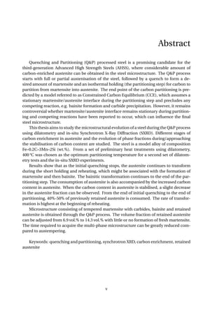
Figure 1.1 known as the “banana diagram” summarises the tensile strength and ten-
sile elongation data for various classes of conventional steels and AHSS. DP steels and
TRIP steels, together with complex phase (CP) steels and martensitic (MART) steels, are
the first generation AHSS. The desire to produce steels with considerably higher strengths
has brought about the development of the second generation AHSS, which are austenitic
steels with high Mn contents [6]. The third Generation AHSS, as forecast by D. Matlock
[7], should exhibit strength-ductility combinations significantly better than the first gen-
eration AHSS while at a cost significantly less than required for second generation AHSS,
and the microstructure consisting of martensite and retained austenite (RA) mixture is sug-
gested [1, 6, 7]. RA is known to enhance the mechanical properties such as ductility in steels
1](https://image.slidesharecdn.com/8b2ffde7-c0f3-47a7-8f34-df7c41853fc3-170201023600/85/MasterThesis-YimingHu-9-320.jpg)
![2 1. Introduction
Figure 1.1: Elongation—tensile strength balance diagram for existing variety of formable steels and prospec-
tive “third-generation” grades. Modified from reference [7].
through the TRIP effect, where the austenite transforms to martensite under a critical stress
or strain and then increase the strain-hardening rate [1]. The volume fraction of RA plays
an important role in the mechanical properties, and typically, higher amount of RA in steels
provides better combinations of strength and elongation [8].
1.2. Q&P Process and CCE
The microstructure consisting of martensite and RA mixture can be achieved using the
quenching and partitioning (Q&P) process developed by Speer et al. [9], which includes
such variants as one-step or two-step Q&P. The partitioning temperature is the same as the
quenching temperature in the one-step Q&P, whereas the partitioning is performed at a
temperature higher than quenching temperature in two-step Q&P.
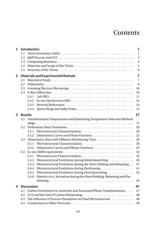
Figure 1.2: Schematic illustration of the Q&P process for producing austenite-containing microstructures.
γ, α1, and α2 represents the austenite, initial martensite and final martensite, respectively. Ci ,Cγ and Cα1
represent the carbon concentrations in the initial alloy, austenite, and martensite, respectively. QT and PT
are the quenching and partitioning temperatures. Adapted from [10].
Figure 1.2 depicts a typical two-step Q&P process. After full austenitisation above the
Ac3 temperature, the steel is quenched to a quenching temperature (QT). At this temper-](https://image.slidesharecdn.com/8b2ffde7-c0f3-47a7-8f34-df7c41853fc3-170201023600/85/MasterThesis-YimingHu-10-320.jpg)
![1.2. Q&P Process and CCE 3
ature, a fraction of martensite referred to as primary martensite (α1) is formed, where the
carbon content in α1 is the same as that in the austenite (γ), and is equal to the carbon con-
tent in the bulk material. Then the steel is held for a short time, followed by a reheating to
the partitioning temperature (PT). During this interval between the initial quenching and
isothermal holding, carbon partitioning and phase transformation are not expected to oc-
cur. In the partitioning step, where the steel is isothermally held for a time, the carbon will
partition from the martensite to the austenite. The driving force for the carbon partition-
ing process is the greater chemical potential of carbon in the supersaturated martensite
than in the austenite, as shown in Figure 1.3. After the partitioning step, a microstructure
of carbon-depleted α1 and carbon-enriched γ will form. If process parameters are cho-
sen properly with the assumption of no carbide precipitation or bainite formation, all the
carbon-enriched γ will be retained at room temperature after final quenching. Otherwise,
a fraction of γ will transform to martensite during final quenching, as shown by α2. To dis-
tinguish from the tempered martensite, the martensite formed during the final quenching
is referred to as fresh martensite. Fresh martensite can increase the brittleness of steels and
therefore is not desirable.
Figure 1.3: Schematic molar Gibbs free energy vs. composition diagrams illustrating metastable equilibrium
at a particular temperature between ferrite and austenite in the Fe-C binary system showing two possible
conditions (I and II) of CCE [11]. α and γ represents the martensite and austenite, respectively. µc is the
chemical potential of carbon and x the carbon content. The CCE condition I or II is denoted by the super-
script I or II.
The end point of the partitioning is marked by the equal chemical potential of carbon
in both phases, referred to as the constrained paraequilibrium (CPE) [9, 11] firstly by Speer
et al. [9]. The term ‘constrained carbon equilibrium’ (CCE) was later proposed by Hillert
and Ågren in place of CPE [12–15]. There are two conditions which are key to CCE:
1. Carbon diffusion is completed when the chemical potential of carbon is equal in the
martensite and austenite phases.
2. The number of iron atoms must be conserved in each phase during the approach to
CCE.
Condition 1 defines the thermodynamic constraint of CCE. Unlike the full equilibrium,
where equilibrium is reached with a unique ferrite and austenite composition at a certain](https://image.slidesharecdn.com/8b2ffde7-c0f3-47a7-8f34-df7c41853fc3-170201023600/85/MasterThesis-YimingHu-11-320.jpg)
![4 1. Introduction
temperature, the CCE is reached with an infinite set of ferrite and austenite compositions.
Condition 2 is the matter balance constraint of CCE and is consistent with the presumption
of a stationary austenite/martensite interface during the partitioning step. This assump-
tion is based on the fact that as Q&P processing is carried out at a relatively low temperature
(350−450 °C), the diffusivities of the substitutional alloying elements are too low to parti-
tion between martensite and austenite.
1.3. Competing Reactions
Condition 2 of CCE has been questioned and many researchers have suggested the
migration of the austenite/martensite interface, either by experiments or by simulations.
Zhong et al.[16] observed that the interfaces of austenite/martensite changed from almost
straight at 480 °C for 3 s to curved structures after increasing the partitioning time to 80 s,
indicating possible movements of iron atoms during the partitioning process. Speer et al.
[17] then examined qualitatively the implications of the mobility of iron atoms at the inter-
face. That is, there will be changes in the volume fraction of austenite and martensite after
the completion of carbon partitioning and repartitioning of carbon atoms might occur as a
result.
Figure 1.4: Schematic tangent intercepts showing ferrite and austenite compositions having equal chemical
potentials for carbon [17].
The theoretical basis for this can be shown in Figure 1.4. Carbon partitioning is con-
sidered to be completed before any interface motion. In the case where the carbon con-
centration in austenite is less than equilibrium (Figure (a)), the iron potential is greater in
austenite than in ferrite, thus creating a driving force for iron atoms to move from austen-
ite to ferrite, indicating an interface migration towards austenite, leading to the growth of
ferrite and the consumption of austenite. In the case where the carbon concentration in
austenite is greater than equilibrium, the iron potential is less in austenite than in ferrite,
and the iron atoms will move from ferrite to austenite, indicating an interface migration
towards ferrite, resulting in the growth of austenite and the consumption of ferrite. There-
fore, the direction of interface movement is controlled by the martensite formation prior
to carbon partitioning, with the phase fractions moving towards their equilibrium values
consistent with the lever rule. Although carbon partitioning is considered to be completed
prior to interface motion due to the greater mobility of carbon atoms at lower tempera-
ture, it should also be noted that any interface movement that occurs will create a need for](https://image.slidesharecdn.com/8b2ffde7-c0f3-47a7-8f34-df7c41853fc3-170201023600/85/MasterThesis-YimingHu-12-320.jpg)
![1.4. Objective and Scope of the Thesis 5
subsequent carbon redistribution, even if carbon partitioning was complete prior to such
movement.
Santofimia et al. [18] later modelled the bidirectional interface migration, and they
have incorporated the influence of interface mobility on the interface migration in their
following work [19]. DeKnijf et al. [20] have observed a clear movement of the austen-
ite/martensite interface in high carbon steel (1wt%) by using in-situ TEM, and compared
the experimental results with the calculated martensite grain width evolution with differ-
ent activation energies using the model proposed in literatures [18, 19]. The comparisons
showed good fit for activation energy between 165 kJ/mol and 170 kJ/mol.
Apart from the possibility of interface migration, bainite transformation [21–23] could
decrease the volume fraction of austenite during the partitioning step and hence the frac-
tion of final retained austenite. In literatures, a faster bainitic transformation with presence
of martensite have been observed than transformation starting with single-phase austenite
[21, 22]. The phase transformation will be accompanied by carbon enrichment in austen-
ite, the mechanism of which is shown in Figure 1.5, where the Gibbs free energy of austenite
is equal to that of bainite on T0 curve. When the carbon concentration of the austenite lies
to the left of the T0 curve, where the Gibbs free energy of bainite is lower, bainite nucle-
ation begins and the excess carbon is rejected into the surrounding austenite, increasing
its carbon content. The enrichment ceases when the austenite composition reaches T0.
Figure 1.5: Schematic molar Gibbs free energy vs. composition, and temperature vs. composition diagrams
illustrating the mechanism of carbon enrichment through formation of carbide-free bainite. Adapted from
[24].
Carbides precipitation [25] in martensite could also happen and therefore reduce the
amount of carbon partitioning into austenite and affect the stability of austenite during
final quenching.
1.4. Objective and Scope of the Thesis
While the in-situ TEM can provide a method to study the local interface mobility, it
failed to determine the impact of the moving interface on the evolution of overall austen-
ite fraction, which will influence the final microstructure. Although dilatometry studies
can help study the evolution of phase fractions, no direct information on the evolution](https://image.slidesharecdn.com/8b2ffde7-c0f3-47a7-8f34-df7c41853fc3-170201023600/85/MasterThesis-YimingHu-13-320.jpg)
![6 1. Introduction
of carbon content can be obtained. There also exists ambiguity in the interpretations of
dilatometry data, e.g. the dilatometric contractions at higher partitioning temperatures
may correspond to reduced ferrite growth, austenite growth, and/or martensite tempering
effects [26]. Synchrotron XRD (SXRD), however, with its in-situ measurement while apply-
ing the thermal cycle, is a technique to study the evolutions of phase fractions and carbon
content simultaneously.
This thesis therefore aims to investigate the microstructural evolution of a steel during
the Q&P process with the help of SXRD. Specifically, the thesis will focus on the change
in the volume fraction and carbon content in austenite during the Q&P process. Different
Q&P cycles are applied and their corresponding microstructural changes are compared. It
is the objective of this thesis to provide experimental proof for the following questions:
• During which stage(s) of the Q&P process will austenite be enriched with carbon?
• Can CCE predict the end point of the carbon partitioning for the studied steel? Will
there be any competing process?
• How can we optimise the steel microstructures (i.e. more RA fraction, higher carbon
content of RA and less fresh martensite)?
1.5. Structure of the Thesis
The remaining part of the thesis consists of the following chapters:
• Chapter 2 presents the studied material, related experimental techniques and proce-
dures of the experiments.
• Chapter 3 presents the results obtained from the experiments.
• Chapter 4 presents the discussions of the results obtained.
• Chapter 5 presents the conclusions and recommendations for future works.](https://image.slidesharecdn.com/8b2ffde7-c0f3-47a7-8f34-df7c41853fc3-170201023600/85/MasterThesis-YimingHu-14-320.jpg)
![2
Materials and Experimental Methods
2.1. Material of Study
The studied material is a hot-rolled steel with chemical composition shown in Table
2.1. Manganese is an austenite stabiliser which retards the formation of ferrite, pearlite,
and bainite; on the other hand, manganese also promotes carbides formation [24]. The
combination of low-carbon and high-silicon contents suppresses the carbide precipitation
during the isothermal holding [27, 28].
Table 2.1: Chemical composition of the studied material
Element C Mn Si Cr P S Al N
Composition (wt.%) 0.2 2.93 1.97 <0.05 <0.002 <0.001 0.009 <0.001
Figure 2.1 shows the banded microstructure of the steel taken from the 6 mm-thickness
slab. The microstructure consists of martensite, bainite and retained austenite (about 12
vol.% determined by XRD). The rolling direction (RD) is also shown in the figure, and the
transverse direction (TD) is vertical to the surface shown in the figure. The banded mi-
Figure 2.1: Microstructure of the as-received material under optical microscopy showing the banded mor-
phology.
7](https://image.slidesharecdn.com/8b2ffde7-c0f3-47a7-8f34-df7c41853fc3-170201023600/85/MasterThesis-YimingHu-15-320.jpg)
![8 2. Materials and Experimental Methods
crostructure results from the segregation of substitutional alloying elements during den-
dritic solidification, leading to Mn-poor region and Mn-rich region. After hot rolling, areas
with different segregation levels will align in the form of bands following the rolling direc-
tion. In the case of Figure 2.1, the high manganese content (higher than 2.5 wt.% [29]) and
the inhomogeneity of manganese result in the banded microstructure.
2.2. Dilatometry
Dilatometry is one of the most powerful techniques for the research on solid-state phase
transformations in steels, since it allows the in-situ monitoring of the dimensional changes
occurring in the sample, which is closely related to the phase transformation and tempera-
ture during the application of thermal cycle [30]. The applicability of dilatometry is due to
the change of the specific volume (the ratio of volume to mass) of a sample during a phase
transformation. When the steel undergoes a phase change, the lattice structure changes,
e.g. from α to γ while heated to the Ac1 temperature.
Figure 2.2: Schematic of the expansion process of a steel and the lever rule. The steel is assumed to be fully
ferritic before the austenisation. [31]
Due to the difference in the atomic volume between α and γ, the phase transforma-
tion will be accompanied by the change in the specific volume, and this would be reflected
as a sudden change in length of the steel, as illustrated by Figure 2.2. When the steel is
heated, it will expand linearly, until it reaches Ac1, where the α → γ transformation starts,
a contraction is expected because of the smaller atomic volume of γ. When the tempera-
ture increases to Ac3, the steel is fully austenitised and a further increase in temperature
will result in the linear expansion of the steel. The transformation temperatures could be
identified around the turning point of the dilatometry curve.
The specimens used for the dilatometry tests are in a cylinder geometry, with diame-
ter of the cross-section equal to 3.55 mm and a length of 10 mm. The heat treatments are
performed in a DIL 805A/D dilatometer either in a vacuum (less than 2.0×10⁻⁴
mbar) or he-
lium atmosphere. Figure 2.3 gives a schematic representation of a dilatometer. The sample
is clamped between two quartz push rods, and a Linear Variable Differential Transformer](https://image.slidesharecdn.com/8b2ffde7-c0f3-47a7-8f34-df7c41853fc3-170201023600/85/MasterThesis-YimingHu-16-320.jpg)
![2.2. Dilatometry 9
is used to record length changes in the sample and the push rods. The specimen is heated
by a high-frequency induction coil, and cooling gas (helium) can be applied through the
small holes in the induction coil. The thermocouple spot-welded on the specimen is used
for temperature record and control. Length resolution of 50 nm can be achieved, and the
temperature resolution is 0.05 °C.
Figure 2.3: Schematic representation of the dilatometer configuration. Adapted from [32].
In order to obtain the transformation temperature, the offset method proposed by Yang
and Bhadeshia [33] is applied. The offset method determines the transformation tempera-
ture with higher accuracy among others and a comparison between these methods can be
seen in reference [33].
Figure 2.4: Schematic of the offset method.
Figure 2.4 gives an example of the determination of Ms through offset method. Firstly,
the data range where austenite contracts linearly is fitted. Then this line is shifted by a value
ε0, which is the strain due to the formation of 1 vol.% martensite, and can be calculated by
Eq. (2.1).](https://image.slidesharecdn.com/8b2ffde7-c0f3-47a7-8f34-df7c41853fc3-170201023600/85/MasterThesis-YimingHu-17-320.jpg)
![10 2. Materials and Experimental Methods
(1+ε0)3
= a−3
γ (2V a3
α +(1−V )a3
γ) (2.1)
where aα and aγ is the lattice parameter of austenite and martensite, respectively, and V
is the volume fraction of martensite, which equals 1% here. The offset line in Figure 2.4 is
therefore shifted upwards by ε0. Ms lies where the experimental data and the offset line
intersect, where in this particular case, Ms = 337.4 °C.
Apart from the determination of transformation temperatures, dilatometry can also be
used to quantitatively determine the amount of transformed phase as a function of tem-
perature using the lever rule as follows [31].
As shown in Figure 2.2, the two dashed lines represent the expansion of pure α and
pure γ with the increase in temperature, respectively. Any point lying on the curved line
in between consists of both α-Fe and γ-Fe. If we draw a line across this point (T , ls) and
intersect with the expansion lines of α-Fe and γ-Fe at (T , lT α) and (T , lT γ), respectively, we
could calculate the volume fraction of α-Fe, fα, as
fα = (ls −lT γ)/(lT α −lT γ) (2.2)
and the details of the derivation for this equation can be seen in reference [31].
2.3. Scanning Electron Microscopy
Scanning electron microscopy (SEM) is used to characterize the microstructures at a
higher magnification compared to optical microscopy. Heat-treated specimens will be cut
in half and then grinded with sand papers, afterwards, they will be polished to a surface
roughness of 1µm. The polished specimens are etched with 2% nital. Before the obser-
vation, the specimens are firstly ultrasonically cleaned with acetone for 2 min, followed by
ultrasonic clean with isopropanol for 2 min. SEM observations were performed using a
JEOL JSM-6500F field emission gun SEM operating at 15 kV.
2.4. X-Ray Diffraction
X-Ray Diffraction is a technique to investigate the fine structure of matter [34]. This
technique can be used to determine crystal structures, the volume fractions of different
phases, chemical analysis and stress measurement.
Planes of atoms within a material will diffract beams of X-rays at specific angles, and
these diffracted beams are commonly used to characterize various material properties.
There are two properties associated with the diffracted beams that are used: the angle be-
tween the incident and diffracted beams (2θ) and the intensity of the diffracted beam (I)
(Figure 2.5).
Bragg’s law relates the angle θ, the wavelength of the beam (λ) and the spacing between
the planes of atoms in the material (d):
nλ = 2dsinθ (2.3)
Furthermore, the intensity of a given diffracted beam is proportional to the volume of ma-
terial that has planes spaced and oriented for diffraction in that particular direction. This
means that the relative volume of phases within a polycrystalline material can be estimated](https://image.slidesharecdn.com/8b2ffde7-c0f3-47a7-8f34-df7c41853fc3-170201023600/85/MasterThesis-YimingHu-18-320.jpg)
![2.4. X-Ray Diffraction 11
Figure 2.5: Schematic representation of Bragg diffraction of crystallographic planes.
from the relative intensities of the diffracted beams [34]. For cubic structures, the spacing d
between certain planes (hkl) is a function of the lattice parameter a and the Miller indices:
d = a/ h2 +k2 +l2 (2.4)
From Eq. (2.3) and Eq. (2.4) we could relate the lattice parameter to the angle between the
incident and diffracted beams. Therefore, from the peak positions of the diffractograms,
the lattice parameter of the cubic structure can be calculated. In the case of steels, since the
lattice parameter of austenite is related to its carbon content, we can calculate the average
carbon content based on the peak positions of the diffractograms.
Hence in this study, XRD is used as a technique to study the volume fraction of austenite
and its carbon content. Lab XRD with X-ray tubes and the synchrotron XRD (SXRD) are
used. The former source of X-ray is widely available in laboratories while the latter can
only be obtained in less than 80 facilities around the world [35].
2.4.1. Lab XRD
Figure 2.6: Schematic of Bragg-Brentano geometry for X-ray tube sources.
Figure 2.6 shows the schematic of the diffractometer using X-ray tube with Bragg-Brentano
geometry. After the sample preparation, the polished sample is then scanned by the Bruker
D8 advanced diffractometer. X-rays are produced by the Co target (with 2 portion of Kα1
and 1 portion of Kα2 radiation), with photon energy of 6.9 KeV [36], wavelength of 1.79 Å](https://image.slidesharecdn.com/8b2ffde7-c0f3-47a7-8f34-df7c41853fc3-170201023600/85/MasterThesis-YimingHu-19-320.jpg)
![12 2. Materials and Experimental Methods
and a penetration depth of 10 µm in steels. During the scanning, the detector position is
recorded as the angle 2θ, and 2θ moves from 40°−135°, with step size of 0.035° and count-
ing time of 4 s for each step. The detector records the number of X-rays observed at each
angle 2θ as count, which is proportional to the intensities.
The obtained diffractograms is analysed in the program MAUD as in Section 2.4.3. [37,
38].
2.4.2. In-situ Synchrotron XRD
Compared to the X-ray tube, synchrotron facilities can produce X-rays with much higher
energies and intensities [39], which allows the X-ray to be transmitted through the materi-
als (1 mm in thickness in this study) and a larger sample volume can be investigated.
Figure 2.7: Schematic of the transmission Geometry for 2D XRD.
The 2D XRD setup as shown in Figure 2.7 is used in the synchrotron in this project,
which enables much faster data acquisition since all the crystalline planes will diffract the
X-rays simultaneously, while in Figure 2.6 the detector needs to rotate in order to record
X-rays diffracted by different planes. If the sample is polycrystalline, the diffraction pattern
will form a series of diffraction cones and each diffraction cone corresponds to the diffrac-
tion from the same family of crystalline planes in all the analysed grains [40]. One cone is
shown in Figure 2.7 and the intersection between the cone and the detector will form a ring
referred to as the Debye-Scherrer ring. Unlike the I − 2θ data acquisition in 1D XRD, the
intensities are recorded in each pixel on the area detector. Azimuthal integration over the
rings are needed for further analysis, which will be discussed later. The faster data acqui-
sition in synchrotron XRD can help study the phase transformations in-situ. In fact, some
set-up can go as fast as 10 Hz.
The Synchrotron X-ray diffraction (SXRD) experiments were performed at the beam-
line ID11 of European Synchrotron Radiation Facility (ESRF). The specimens are in a typ-
ical tensile specimen geometry (dog-bone shape), as shown in Figure 2.8(a), with an over-
all length of 40 mm, shoulder length of 10 mm on both sides and a gage cross-section of
1×1 mm2
. The Electrothermal Mechanical Testing (ETMT) System was applied for the ther-
mal cycle during the in-situ XRD experiments. Compared to the dilatometry tests where
the steels are heated by the induction coil, heating is achieved by passing direct current](https://image.slidesharecdn.com/8b2ffde7-c0f3-47a7-8f34-df7c41853fc3-170201023600/85/MasterThesis-YimingHu-20-320.jpg)
![2.4. X-Ray Diffraction 13
through the gauge length of the specimen controlled by a Pt/Pt-13% Rh thermocouple spot-
welded to the centre of the gauge length. Argon was used to minimise sample oxidation.
Figure 2.8: (a) A schematic of the specimen showing the area of exposure for SXRD measurements, the beam
size is 200 × 200 mm2
. Also shown is the CeO2 powder attached on top of the specimen for calibration. (b) A
schematic of the diffraction measurement set-up. the Debye-Scherrer rings are shown on the area detector.
Figure 2.8 presents the schematic of the experimental setup for the measurement. The
incident beam has a wavelength λ = 0.15582 Å (79.57 keV), and the sample to detector dis-
tance is about D = 300 mm. The diffracted beams were recorded by the Frelon CCD camera,
which has an image resolution of 2048×2048 pixels and a pixel size of 50×50 µm2
. Before
the in-situ measurement of each specimen, a standard material (CeO2) was measured for
later calibration of the system configuration, e.g. beam center, sample-detector distance
and tilted angle of the detector. The time of exposure was 60 s for the CeO2. During the
thermal cycle, the ETMT was run under load control with a set point of zero load to permit
free thermal expansion of the sample. The exposure time was 0.1 s for the steel specimens.
Including data recording time, powder diffraction rings were therefore recorded at ∼0.7 s
intervals.
The 2D XRD patterns as in Figure 2.8 need to be reduced to the standard 1D I−2θ profile
for further analysis. However, before the data reduction, calibration for the system config-
uration (e.g. sample-detector distance, tilt angle of the area detector, etc.) is required. The
calibration process can be referred in literature [41] and the calibrated results for each spec-
imen are shown in Table B.1 (see Appendix B.2). The data reduction was performed with
the program Fit2D [42, 43] developed at ESRF with system calibration, dark current sub-
traction, flat field correction and spatial distortion correction. As introduced before, every
pixel in the area detector is 50×50 µm2
in size, and therefore, a pixel (Column, Row) could
have a position (x, y) in the Cartesian coordinate system, and
x = 50Column
y = 50Row
(2.5)](https://image.slidesharecdn.com/8b2ffde7-c0f3-47a7-8f34-df7c41853fc3-170201023600/85/MasterThesis-YimingHu-21-320.jpg)
![14 2. Materials and Experimental Methods
For the azimuthal integration, the polar coordinate system should be used. A point
(x, y) in the Cartesian coordinate system can be transformed into a point (r,ϕ) into the
polar coordinates according to:
r = x
2
+ y2
ϕ = tan−1
(y/x)
(2.6)
For every point (r, ϕ) in the area detector, an intensity value I(r, ϕ) is recorded, and
for the same radius r, we could integrate over the whole azimuthal range from 0 to 2π to
obtain the relationship between the integrated intensity I(r) and the radius r:
I(r) =
2π
0
I(r,ϕ)dϕ (2.7)
According to the relationship between the r and 2θ, we could transform the I −r relation-
ship to I −2θ relationship:
I(r)
r=D tan2θ
−−−−−−−→ I(2θ) (2.8)
2.4.3. Rietveld Refinement
Both the integrated diffraction patterns from SXRD and the 1D diffractograms obtained
by lab XRD are analysed with the Rietveld refinement software MAUD [37, 38]. The refine-
ment works by minimizing the weighted sum of squares W SS:
W SS =
i=N
i=1
wi (Iobs,i − Icalc,i )2
(2.9)
where Iobs,i and Icalc,i is the ith observed and calculated intensity respectively. wi is the
weight assigned to the ith sum of square, and for a standard x-ray powder diffraction pat-
tern, wi = 1/Icalc,i [44]. For minimizing the W SS, the Levenberg-Marquardt Algorithm
[45, 46] is implemented in MAUD. The weighted profile R-factor Rwp [47], following di-
rectly from the square root of the W SS minimized and scaled by the weighted intensities,
is a parameter to assess the quality of the refinement, and
Rwp =
Σi=N
i=1
(Iobs,i − Icalc,i )2
i=N
i=1 wi I2
obs,i
(2.10)
Lutterotti [48] suggested that a good refinement for the cubic crystal structures would have
a Rwp value less than 8%, while Toby [47] shows that Rwp value as a criterion for a good
fitting is only suitable for low background levels.
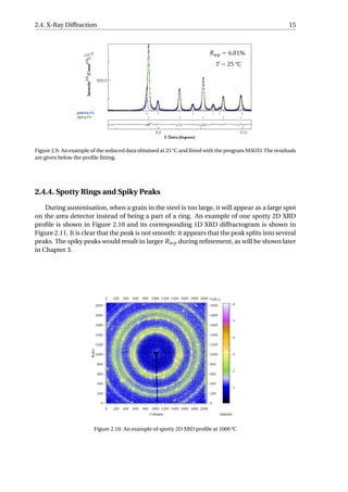
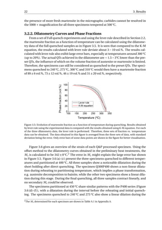
An example of the fitted I −2θ profile is presented in Figure 2.9. Very low background
level exists in the diffractogram and the Rwp is 6.01%, showing a good quality of fitting. The
austenite (gamma-Fe in the figure) profile and ferrite (alpha-Fe in the figure) profile are
shown separately and their peak positions are represented by the tick below the fitted pro-
file. The volume fraction and lattice parameter of each phase can be extracted from each
fitted profile, which helps to study the evolution of phase fractions and carbon content.](https://image.slidesharecdn.com/8b2ffde7-c0f3-47a7-8f34-df7c41853fc3-170201023600/85/MasterThesis-YimingHu-22-320.jpg)
![3
Results
3.1. Transformation Temperatures and Quenching Tempera-
ture Selection Methodology
In order to select the austenitising temperature, quenching temperature and partition-
ing temperature, it is necessary to estimate the Ac1, Ac3, Ms and Bs temperature using em-
pirical equations. The Ac1, Ac3, Ms and Bs [49–52] temperature are calculated as follows:
Ac1(°C) = 723−16.9(wt.%Ni)+29.1(wt.%Si)+6.38(wt.%W)
−10.7(wt.%Mn)+16.9(wt.%Cr)+290(wt.%As)
= 749.1
(3.1)
Ac3(°C) = 955−350(wt.%C)−25(wt.%Mn)+51(wt.%Si)
+106(wt.%Nb)+100(wt.%Ti)+68(wt.%Al)−11(wt.%Cr)
−33(wt.%Ni)−16(wt.%Cu)+67(wt.%Mo)
= 912.0
(3.2)
Ms(°C) = 462−273(wt.%C)−26(wt.%Mn)
−16(wt.%Ni)−13(wt.%Cr)−30(wt.%Mo)
= 329.4
(3.3)
Bs(°C) = 656−57.7(wt.%C)−75(wt.%Si)−35(wt.%Mn)
−15.3(wt.%Ni)−34(wt.%Cr)−41.2(wt.%Mo)
= 389.5
(3.4)
The calculated Ms and Bs using Eq. (3.3) and Eq. (3.4) are close to the findings of Bhadeshia
[53] for the Fe–3Mn–2Si–C (wt.%) series steels considering the error bars in Figure 3.1, from
which it is shown that when carbon content is 0.2 wt.%, Ms = 357 ± 20 °C and Bs = 427 ± 20 °C.
However, for more precise determinations of transformation start temperatures, in-situ ex-
periments such as dilatometry should be performed.
17](https://image.slidesharecdn.com/8b2ffde7-c0f3-47a7-8f34-df7c41853fc3-170201023600/85/MasterThesis-YimingHu-25-320.jpg)
![18 3. Results
Figure 3.1: Calculated transformation start temperatures in Fe–2Si–3Mn steel as function of carbon concen-
tration [53].
Before the heat treatment, a model [12] based on the Koistinen-Marburger (K-M) equa-
tion [54] was used for both quenching temperature selection and the estimation of RA
fraction at a given quenching temperature. In this model, the volume fraction of primary
martensite is firstly calculated using the K-M equation:
fα1
= 1−exp(−β(Ms −Tq)) (3.5)
where fα1
is the volume fraction of primary martensite and Tq the temperature to which
the steel is quenched. The parameters β depends on the chemical composition [51] of the
steel according to:
β = 0.0224−0.0107(wt.%C)−0.0007(wt.%Mn)
−0.00005(wt.%Ni)−0.00012(wt.%Cr)−0.0001(wt.%Mo)
(3.6)
According to Eq. (3.6), the parameter β is calculated to be 0.01816. By substituting the value
of Ms and β into Eq. (3.5), the evolution of martensite volume fraction during quenching is
obtained as in Figure 3.2 (a).
The model assumes full partitioning and precludes any competing reactions. There-
fore, no phase transformation is expected before or during the partitioning step, and all
the carbon atoms in the primary martensite are assumed to partition completely into the
austenite. With this assumption, we can obtain the carbon content in austenite (Cγ) at
the end of carbon partitioning from the matter balance of carbon atoms before and after
partitioning:
Ci = (1− fα1
)Cγ (3.7)
where Ci is the carbon content in the bulk material. Since the carbon content in austenite
has changed after the partitioning step, a secondary martensite-start temperature Ms2 can
thus be calculated using Eq. (3.3) again. Similarly, the parameter β should be recalculated
according to the enriched carbon content in austenite.
There exists an optimum QT according to this model. Below this temperature, too much
austenite is consumed during initial quenching. Above this temperature, the carbon par-
titioning into austenite is not enough to stabilise the austenite, resulting in the formation](https://image.slidesharecdn.com/8b2ffde7-c0f3-47a7-8f34-df7c41853fc3-170201023600/85/MasterThesis-YimingHu-26-320.jpg)
![3.1. Transformation Temperatures and Quenching Temperature Selection Methodology 19
of fresh martensite during the final quenching, thus decreasing the fraction of RA. This
optimum temperature T0 is obtained when no fresh martensite will form during the final
quenching, which requires
Ms2 = 25 (3.8)
T0 can be solved using Eq. (3.3), Eq. (3.7) and Eq. (3.8). If Tq ≤ T0, the austenite obtained af-
ter initial quenching can be fully retained after the final quenching. Therefore, the volume
fraction of RA (fγr ) would only depend on fα1
:
fγr = 1− fα1
(3.9)
If Tq > T0, the fraction of fresh martensite (fα2
) formed during final quenching needs to be
considered, which can be obtained by applying Eq. (3.5) again:
fα2
= (1−exp(−β2(Ms2 −25)))(1− fα1
) (3.10)
It should be noted that the K-M equation in Eq. (3.10) is applied to the volume fraction of
austenite at the end of the initial quenching, i.e. 1− fα1
. Also, the quenching temperature
is set to be 25 °C. Therefore, the volume fraction of RA can be obtained as:
fγr = 1− fα1
− fα2
(3.11)
Following the steps from Eq. (3.5) to Eq. (3.11), we can obtain the relationship between the
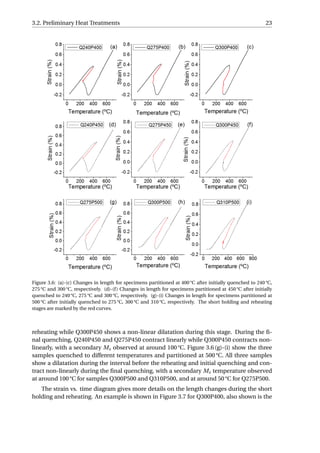
volume fraction of RA and the quenching temperature as in Figure 3.2. The maximum vol-
ume fraction of RA is estimated to be around 15.2 vol.% when initially quenched to 225.7 °C.
However, it should be noted that this methodology is simplified with the assumption of full
partitioning and exclusion of competing processes that may happen during the Q&P pro-
cess, e.g. bainite formation and carbide precipitation. The influence of carbon partitioning
kinetics [55] is also not taken into consideration.
Figure 3.2: (a) Evolution of Martensite fraction as a function of temperature during quenching calculated
using the K-M equation. (b) Prediction of RA fraction with different quenching temperatures applied using
the methodology in reference [12].](https://image.slidesharecdn.com/8b2ffde7-c0f3-47a7-8f34-df7c41853fc3-170201023600/85/MasterThesis-YimingHu-27-320.jpg)
![26 3. Results
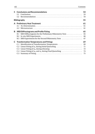
An example was given in Figure 3.9. The linear contraction of austenite during the full
quench is fitted, and the difference between the experimental value and the fitted value is
calculated as the net dilation due to formation of martensite, which equals 0.90%. Accord-
ing to XRD, the volume fraction of retained austenite in the fully-quenched specimen is
approximately 1%. Hence, the net dilation of 0.90% would correspond to the formation of
99% martensite. Similarly, the net dilation due to martensitic transformation of Q300P500
can be calculated to be 0.13%, which is associated with the formation of 14.3% martensite.
Since linear contraction is observed during the final quenching for the P400 series as well
as Q240P450 and Q275P450, they will have no fresh martensite in the microstructure. fα2
is calculated to be 4.4%, 5.8% and 16.7% for Q300P450, Q275P500 and Q310P500, respec-
tively. The error in calculating fα2
is estimated to be around 10% of the fα2
value. This error
is due to the variability in the selection of data from quenching curves for linear fitting.
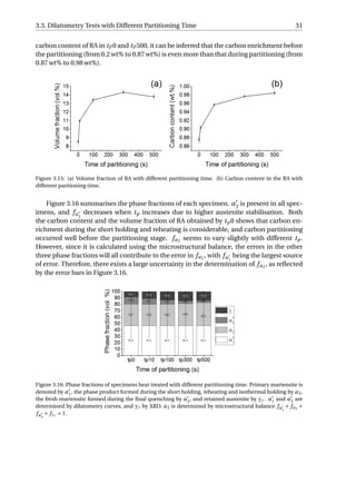
For the determination of fγr , lab XRD experiments were performed. The obtained diffrac-
tograms are summarised in Appendix B.1 and they are fitted using MAUD as described in
Section 2.4.3. From the program MAUD, the volume fraction of RA and lattice parameter of
austenite aγ can be extracted. aγ can be related to the chemical compositions according to
[56]:
aγ = 3.556+0.0453xC +0.00095xMn +0.0056xAl (3.13)
where xC , xMn and xAl represent the weight percentage of C, Mn and Al in austenite, re-
spectively. xC can therefore be calculated through Eq. (3.13).
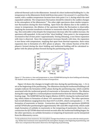
Figure 3.10: (a) The volume fraction of RA for different Q&P processed specimens. (b) The carbon content of
RA for different Q&P processed specimens.
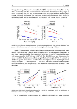
The volume fraction and the carbon content of RA are shown in Figure 3.10. The highest
amount of RA (13.6 vol.%) was obtained for Q300P400. The P500 series retained the least
austenite in the microstructure, ranging from 2.0 vol.% to 4.0 vol.%. As for the carbon con-
tent in the specimens, around 1.00 wt% is determined for the P400 series, around 0.90 wt%
for the P450 series, and ranging from 0.75 wt% to 0.87 wt% for the P500 series.
Now that fα1
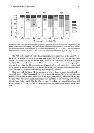
, fα2
and fγr for each specimen are known, fα2 can be computed for each
specimen. The results are shown in Figure 3.11, with phase fraction of each specimen. The
error in calculating fα2 depends on the errors of other phase fractions, and since the error
in fα1
is much larger than the error in fα2
and that in fγr , the error in calculating fα2 is
almost the same as the error in fα1
[57].](https://image.slidesharecdn.com/8b2ffde7-c0f3-47a7-8f34-df7c41853fc3-170201023600/85/MasterThesis-YimingHu-34-320.jpg)
![28 3. Results
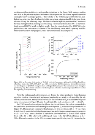
3.3. Dilatometry Tests with Different Partitioning Time
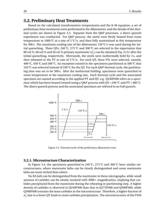
Figure 3.12: Thermal cycle of the dilatometry tests with different partitioning time.
In order to study the effect of partitioning time (tp) on the final microstructure, a set
of dilatometry tests with different partitioning time is designed. 300 °C and 400 °C are se-
lected for QT and PT, respectively, since with the two parameters, the steel had a higher
amount of RA and also higher carbon content in RA. At 400 °C, different partitioning time is
selected, namely, 0 s, 10 s, 100 s, 300 s and 500 s. Separate from the Q&P processes, a spec-
imen is fully quenched, and the specimen and the process are named as Full quench. The
Q&P processes and associated specimens are named according to the partitioning time,
e.g. tp10 signifies a Q&P process with a partitioning time of 10 s, or specimen partitioned
with 10 s. The aim of tp0 is to investigate to what carbon content will the RA be enriched
when the steel is just heated to 400 °C, without any time of holding.
The details of the thermal cycles are shown in Figure 3.12. A cooling rate of 31.5 °C/s is
chosen instead of the maximum value in order to reduce temperature fluctuation after the
initial quenching. The short holding time is reduced to 3 s. Other process parameters are
the same as in the preliminary heat treatments.
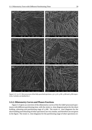
3.3.1. Microstructural Characterization
The aim of the SEM is to study when the carbides precipitated during the Q&P process.
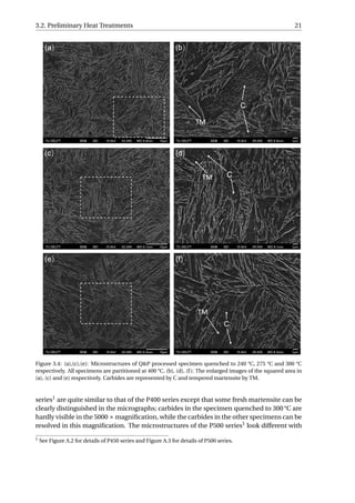
Figure 3.13 presents the SEM micrographs of all the specimens. The carbides observed
in the fully quenched specimen should arise from auto-tempering, which refers to a pro-
cess where the martensite formed near the Ms gets tempered during the remainder of the
quench [24]. Small quantity of carbides have been resolved in all the specimens, implying
that the carbides already precipitate during reheating from QT to PT. As the time of par-
titioning increases, no obvious increase in the quantity of carbides can be distinguished
among the five Q&P processed specimens. The partitioning step can therefore be regarded
as a process without further carbides precipitation at 400 °C.](https://image.slidesharecdn.com/8b2ffde7-c0f3-47a7-8f34-df7c41853fc3-170201023600/85/MasterThesis-YimingHu-36-320.jpg)
![32 3. Results
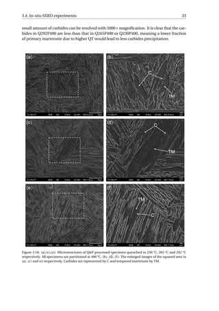
3.4. In-situ SXRD experiments
The above two sections give information about how fα1
and tp influence the final mi-
crostructure of the steels. However, it is not known how the microstructure evolved during
the Q&P process. In this section, a set of heat treatments were performed with the in-situ
XRD scanning to study the microstructural evolution during the Q&P process. The process
parameters are selected based on the results of the preliminary heat treatments. Similarly,
PT is selected to be 400 °C as most carbon partitioning is expected, stabilising RA. QTs 240,
275 and 300 °C were initially selected, although 8 − 10°C lower than the preset QTs were
achieved experimentally. Figure 3.17 depicts the details of the thermal cycles applied, with
the actual QTs in place of the preset ones.
Figure 3.17: Thermal cycle of the in-situ SXRD experiments.
The obtained 2D XRD profiles were firstly reduced into 1D diffractograms using Fit2D,
followed by Rietveld refinement using MAUD. For the sake of simplicity, martensite, bainite
and ferrite are treated as one BCC phase (α) during the Rietveld refinement. Both data
reduction and refinement started from the beginning of the initial quenching to the end of
the final quenching for each specimen, and the Rwp values for the refinement are given in
Figure B.3 (see Appendix B.2). Higher Rwp values were obtained for the initial quenching
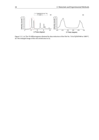
files since their peak profiles are less smooth (Figure 2.11). The reason for the spiky profile is
that during austenisation, some of the austenite grains grow preferably and their large grain
size cannot be considered as “powder” thereafter. Instead of contributing to the Debye-
Scherrer rings, the large grain will appear as a large spot (Figure 2.10) on the area detector
[58]. Error bars in this part are estimated from the program MAUD, or calculated based on
the estimation of MAUD.
3.4.1. Microstructure Characterization
The microstructures of the Q&P processed specimens after the in-situ SXRD experi-
ments are shown in Figure 3.18. The microstructures of specimens quenched to 230 °C,
265 °C and 292 °C look quite similar, consisting of martensite that responded to the 2% ni-
tal etching in two different ways since some martensite laths are clearly more etched than
others. No RA lath can be distinguished from the martensite in these micrographs, while](https://image.slidesharecdn.com/8b2ffde7-c0f3-47a7-8f34-df7c41853fc3-170201023600/85/MasterThesis-YimingHu-40-320.jpg)
![34 3. Results
3.4.2. Microstructural Evolutions during Initial Quenching
From the diffractograms (Figure 3.19) of the four specimens, it is found that some small
fraction of α formed at 803 °C, 807 °C, 709 °C and 816 °C for full quench, Q230P400, Q265P400,
Q292P400, respectively. This temperature range (709−816 °C) is far above the Ms or Bs tem-
perature of the material, and therefore, the ferrite formed at these temperatures could not
be martensite or bainite. This temperature range (709 − 816 °C) is close to the Ae3 tem-
perature of the material (818 °C calculated by the Andrews Equation [49]). Since the Wid-
manstätten ferrite grows at a temperature in proximity to the Ae3 [59, 60], the ferrite formed
high above the Ms or Bs is considered to be Widmanstätten ferrite.
Figure 3.19: XRD diffractograms showing the first observation of ferrite peaks for specimen Full quench,
Q230P400, Q265P400 and Q292P400 in the in-situ XRD experiments, respectively.
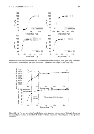
Figure 3.20 presents the evolution of austenite volume fraction (fγ) for the four speci-
mens during the full quench or initial quenching. The shape of the four curves resemble
the “S”-shaped curve in Figure 3.5 determined by the lever rule, even though the austenite
transformed well before the Ms in all four specimens. By examining both the evolution of
austenite volume fraction and the change in the length of the specimen as measured by
the ETMT, we can determine when the fast decomposition of austenite begins. Figure 3.21
compares the rate in length change with the phase evolution of the specimen Q292P400.
The rate of length change firstly stabilised at around 0.0003 when quenching from 1000 °C
to 420 °C, during which the austenite transformed slowly by a volume fraction of about 7%.
Then a sudden decrease in the rate of contraction can be observed in Figure 3.21 (a), which
corresponds to a fast γ to α transformation. This has also been observed in Figure 3.21 (b)
by a much faster decrease in the volume fraction of austenite (7% when quenching from
420 °C to 390 °C compared to 7% when quenching from 1000 °C to 420 °C).](https://image.slidesharecdn.com/8b2ffde7-c0f3-47a7-8f34-df7c41853fc3-170201023600/85/MasterThesis-YimingHu-42-320.jpg)
![36 3. Results
However, this temperature is higher than the Ms (342 ± 8°C) determined in Section
3.2.2 and close to the Bs. Therefore, the 420 °C should be identified as the Bs for specimen
Q292P400. Similarly, Bs has been identified for the other three specimens as in Appendix
C.1. The phase compositions can therefore be obtained as in Figure 3.22.
Similar amount (5.0−6.6 vol.%) of Widmanstätten ferrite (αW ) formed for Q292P400
and Q265P400 during the initial quenching, while αW is higher for Q230P400. The amount
of bainite formed ranges from 15.7 to 23.4 vol.%. Due to more formation of Widmanstätten
ferrite and bainite before cooling to Ms, Q275P400 has almost the same amount of primary
martensite as Q230P400. But still, the amount of austenite decreases with the QT.
Figure 3.22: Phase fractions of specimens quenched to different temperature and partitioned at 400 °C. Wid-
manstätten ferrite is denoted by αW , bainite by αb, primary martensite by α1 and austenite by γ.
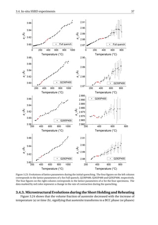
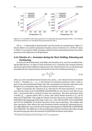
Figure 3.23 gives an overview of the changes in lattice parameters during initial quench-
ing for the four specimens. aγ represents the lattice parameter of austenite and aα the lat-
tice parameter of ferrite. The lattice parameters of austenite are shown in the left column of
Figure 3.23, where a decrease in the rate of contraction during quenching can be observed
for all four specimens at around 400 °C, represented by the red data points. The decrease in
the rate of contraction stopped at around 300 °C for Full quench, Q230P400 and Q265P400
while it stopped at 389 °C for Q292P400. An increase in the rate of contraction is observed
in the corresponding temperature range for ferrite, as represented by the red data points in
the right column of Figure 3.23. The observed phenomena should be related to the marten-
sitic transformation since it has been reported that during standard quenching process, the
martensite phase should be subject to tensile stress and the austenite should be in stress of
the opposite sign (compressive stress) to satisfy the force balance [61].
The error bar of aγ is within the size of the data point (< 5×10⁻⁴
Å), while the large error
bar of aα at higher temperatures is due to the small volume fraction of α at these tempera-
tures. Despite the small error of aγ, there is an observable scatter from linear contraction at
temperature range 700–1000 °C. The scatter may result from the spotty rings observed dur-
ing the 2D diffractograms in this temperature range (Figure 2.10 and 2.11). The spotty rings
will result in less smooth peak profiles and thus errors in the determination of aγ. However,
this is not reflected in the error bar of aγ determined by the program MAUD, since the error
bar is only estimated from the fitting in the program; the spikes that appear in the peak
profiles are not taken into considerations.](https://image.slidesharecdn.com/8b2ffde7-c0f3-47a7-8f34-df7c41853fc3-170201023600/85/MasterThesis-YimingHu-44-320.jpg)
![3.4. In-situ SXRD experiments 39
rate of ∼ 4×10⁻⁵
can be extracted for aα. However, from this linear expansion, it is not pos-
sible to calculate the amount of carbon partitioned away from the BCC phase. This might
result from the fact that in the current work, martensite, bainite and ferrite are treated as α
to simplify the Rietveld refinement process. The determination of the peak positions and
thus aα is less accurate since the α peak is composed of peaks of martensite, bainite and
ferrite. Therefore, only aγ will be used for the quantification of carbon content.
The non-linear increase of aγ with increasing temperature during reheating could be
contributed from three processes: the thermal expansion during reheating, the release of
stress from the previous martensitic transformation [61] and carbon atoms partitioning
from the BCC phase into austenite.
Figure 3.26: (a) aγ of Q230P400 during initial quenching and reheating. (b) aγ of Q265P400 during initial
quenching and reheating. (c) aγ of Q292P400 during initial quenching and reheating. The linear part of the
data in initial quenching is fitted for each specimen.
Figure 3.26 (a) shows the evolution of aγ for specimen Q230P400 quenched to 230 °C
and then reheated to 400 °C, which presents more clearly the influence of the three con-
tributions on aγ during reheating. The error bars of both the initial quenching data and
reheating data are within the size of the data points (< 5 × 10⁻⁴
Å). The data in the initial
quenching curve (a
quench
γ ) before the martensitic transformation is fitted linearly, repre-
sented by the blue line in the figure and referred to as a
f it
γ . This line represents the dilation
or contraction of austenite without strain or carbon partitioning process. The details of
the fitting are given in Figure C.4-C.6 and the results are summarised in Table C.2. Once
the martensitic transformation occurs, the difference between the blue line and the black
data point can be considered as the contraction of aγ due to the transformation stress. The
expansion of aγ during reheating is represented by the red data point (areheat
γ ) in the fig-
ure, and as temperature increases, areheat
γ soon intercepts with the fitted line at point E.
When the temperature is further increased, areheat
γ is greater than a
f it
γ , implying that the
carbon partitioning and/or stress release have compensated for the contraction induced
by martensitic transformation. If there is stress release but no carbon partitioning before
heating to point E, then the stress release and thermal expansion contribute to the increase
of areheat
γ . At point E, the stress release can be considered to be complete and therefore fur-
ther increase of areheat
γ is due to carbon partitioning into austenite and thermal expansion.](https://image.slidesharecdn.com/8b2ffde7-c0f3-47a7-8f34-df7c41853fc3-170201023600/85/MasterThesis-YimingHu-47-320.jpg)
![40 3. Results
If there is carbon partitioning and stress release before heating to point E, then carbon par-
titioning started early during reheating. Therefore, in the area right to point E, the austenite
has been enriched by carbon regardless of how stress is released.
Since it is unknown how the transformation stress is released during the reheating, the
data presented is not sufficient to calculate the evolution of carbon content in austenite
during reheating. But still, we can estimate the the amount of carbon enriched through
the isothermal holding by calculating the carbon content at the beginning and the end of
reheating:
• beginning of reheating: stress has not been released and no carbon enrichment oc-
curred. The carbon content can be calculated using Eq. (3.13) after extrapolating the
fitted line to T = 25°C.
• end of reheating: the stress is assumed to be completely released at this point, the dif-
ference between areheat
γ and a
f it
γ can be regarded as the expansion due to the carbon
enrichment. The carbon content can be calculated by Eq. (3.13) through the areheat
γ
at room temperature (areheat
γ−RT ), which can be expressed by:
areheat
γ−RT = areheat
γ−T −k f it
(T −25) (3.14)
where areheat
γ−T is the lattice parameter of austenite at temperature T during reheating
and k the slope of the fitted line. The k value is shown in Table C.2.
Therefore, for Q230P400:
• beginning of reheating: T = 230°C, areheat
γ = 3.5942 ± 0.0005Å, the corresponding
areheat
γ at room temperature can be calculated by extrapolating the fitted line to room
temperature and areheat
γ−RT = 3.5784±0.0007Å. The carbon content thus can be calcu-
lated with Eq. (3.13) and Creheat
γ−T =230 = 0.43±0.02 wt%.
• end of reheating: T = 400°C, areheat
γ = 3.6208 ± 0.0005 Å, and substituting this into
Eq. (3.14), the corresponding areheat
γ at room temperature can be calculated to be
areheat
γ−RT = 3.5892 ± 0.0007Å, similarly, with Eq. (3.13), the corresponding carbon con-
tent is Creheat
γ−T =400 = 0.67±0.02 wt%4
. Hence, the carbon content in austenite increased
by 0.24±0.03 wt%5
during the reheating process.
Similarly, to calculate the changes in the carbon content during reheating for the other
two specimens, Figure 3.26 (b) and Figure 3.26 (c) are presented. The results are sum-
marised in Table 3.1. The carbon content in austenite of Q265P400 and Q292P400 increased
by 0.17±0.06 wt.% and 0.17±0.04 wt.%, respectively, during the reheating process. It is no-
table that the carbon content at the beginning of reheating is higher than 0.20 wt.%. One
reason for this is that the formation of αb and αW during initial quenching can enrich the
austenite. The choice of empirical equation (Eq. 3.13) might also result in the deviation
from 0.20 wt.%.
4
The error (δ) of kx +b equals (kδx)2 +(δb)2 if variable x and b are independent [57]. Since k here is the
fitted slope in Table C.2, which is very small (in the order of 10−5
), the error of kx +b would be δb, which is
the error of the fitted intercept in Table C.2
5
The error (δ) of a −b equals (δa)2 +(δb)2 if variable a and b are independent [57].](https://image.slidesharecdn.com/8b2ffde7-c0f3-47a7-8f34-df7c41853fc3-170201023600/85/MasterThesis-YimingHu-48-320.jpg)
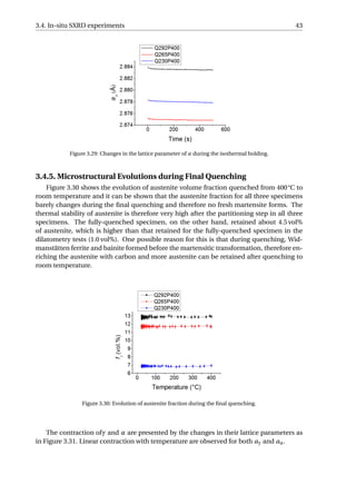
![3.4. In-situ SXRD experiments 45
Figure 3.32: (a) The transformed fraction of austenite with time. (b) The rate of transformation as a function
of the transformed fraction of austenite. t = 0 is selected at the end of the initial quenching for each specimen.
In order to know how the rate of α2 formation changes with the phase transformation
proceeding, the data in Figure 3.32 (a) is firstly smoothed using the adjacent-averaging
method [62] to reduce the scattering of the data. Afterwards, the first derivative of f n
α2
is
taken with respect to t, as shown in Figure 3.32 (b). For all three specimens, the fastest
rate of α2 formation occurs at the beginning of reheating, and with the transformation pro-
ceeding, the rate of transformation will decrease and then increase, and this turning point
corresponds to f n
α2
= 10% for each specimen. The corresponding temperature is higher for
specimens with a higher volume fraction of austenite at the beginning of this stage: 247 °C,
289 °C and 302 °C for Q230P400, Q265P400 and Q292P400 respectively. For Q230P400 and
Q265P400, the rate of α2 formation increases until 20% of transformation is reached, fol-
lowed by a decrease in rate. For Q300P400, the rate continues to increase until 25% of
transformation is reached, and then decreases until the partitioning is finished. Although
the rate of Q292P400 decreases, it is still higher than that of Q265P400 and Q230P400 dur-
ing the partitioning step. This difference is enlarged after f n
α2
= 30%, where higher f n
α2
is
expected for Q292P400.](https://image.slidesharecdn.com/8b2ffde7-c0f3-47a7-8f34-df7c41853fc3-170201023600/85/MasterThesis-YimingHu-53-320.jpg)

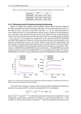
![4
Discussions
4.1. Carbon Enrichment in Austenite and Associated Phase Trans-
formations
Both the dilatometry and SXRD experiments show that austenite can be enriched with
carbon through the reheating and partitioning steps, with more carbon enrichment in austen-
ite during reheating than the partitioning step. The carbon enrichment is accompanied by
the consumption of austenite and the formation of a BCC phase or phases (α2). α2 formed
immediately after the initial quenching stops. Since this process starts from below Ms to
above Ms, it is difficult to determine whether α2 consists of bainite, martensite, or both.
Above Ms, researchers [63–69] agree that the isothermal products formed from the de-
composition of austenite consists of bainitic ferrite with or without carbides and retained
austenite. The bainitic transformation will also be accelerated by the primary martensite
formed before the isothermal treatment, because the martensite-austenite interfaces act as
additional potential nucleation sites [21]. Since partitioning is performed at 400 °C, which
is within the bainitic temperature range, α2 formed during the partitioning step should be
bainite (αb). However, controversy exists over the isothermal products formed below Ms,
which can be purely bainitic [27, 66, 70], martensitic [71], or a phase product neither purely
martensitic nor bainitic [69, 72, 73]. The kinetics analysis in Section 3.4.6 suggests that α2
might form in two stages during reheating, since the rate of transformation firstly decreased
and then increased during reheating. The stage during which the rate of transformation de-
creased might correspond to the slowing martensite formation. When the initial quench-
ing stoped and reheating started, the martensite continued to form at a fast rate, however,
with the carbon partitioning into austenite, Ms is lowered while the steel is reheated. The
lowering Ms and the rising temperature decreases the undercooling until the undercool-
ing is not enough to continue the martensite formation (corresponding to the first turning
point in Figure 3.32). The stage during which the rate of transformation increased might
correspond to the bainite formation. The bainitic transformation then continued until the
end of partitioning with a decreasing rate of transformation. The parabolic relationship
between the rate of bainitic transformation and the phase fraction might be explained by
the model in literatures [74, 75]. With the presence of some fraction of primary martensite
fα1
, the rate of isothermal bainitic transformation d fαb
/dt is related to the volume fraction
47](https://image.slidesharecdn.com/8b2ffde7-c0f3-47a7-8f34-df7c41853fc3-170201023600/85/MasterThesis-YimingHu-55-320.jpg)
![48 4. Discussions
of bainite fαb
as:
d fαb
dt
= (1− fαb
− fα1
)(1+λαb
fαb
+λα1
fα1
)κ (4.1)
where λαb
and λα1
is the autocatalytic constant due to the presence of bainite and pri-
mary martensite, respectively. κ is a rate constant which is related to temperature. At a
given temperature and certain fαb
range, d fαb
/dt will have a parabolic relationship with
fαb
, i.e. d fαb
/dt increases with fαb
to a maximal point and then decreases. However, in
our case, part of the curve does not reside in the isothermal region. Moreover, it is not
known whether the inhomogeneity of manganese might result in the observed kinetics of
phase transformation, since austenite stability in the Mn-rich region is higher than that in
the Mn-poor region. Therefore, the analysis above is only qualitative and simplified. For
more precise phases determination and quantification, characterization techniques such
as TEM, EBSD and IF spectrum can be used [69, 72, 73].
4.2. CCE and the End of Carbon Partitioning
Due to the formation of α2, the CCE model cannot be used for the prediction of the
end of partitioning for the studied steel since it precludes any competing reactions dur-
ing carbon partitioning. The model in literature [74, 75] might provide a better method to
simulate the phase transformations of the studied steel. The coupling of carbon partition-
ing process and bainite formation is included in the model. However, this model does not
take into account the carbon partitioning and bainite formation during reheating; both of
the processes are assumed to occur only during the partitioning step. As the results show
that the rate of transformation is fastest at the start of reheating, and as many researchers
[27, 66, 69, 70, 70–73] have observed the immediate phase transformation after the initial
quenching, the phase transformations during reheating as well as the short holding before
the partitioning step should not be ignored.
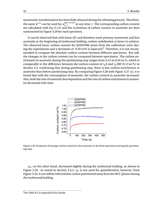
As Figure 3.28 shows, Cγ of Q230P400 firstly reached a plateau at around t = 150 s, and
the stabilisation kept for about 50 s, followed by a slight decrease in Cγ. Cγ in Q265P400
increased until t = 300 s and stayed constant afterwards for 200 s. Cγ of Q292P400 contin-
ued to increase until the end of the partitioning step, showing a growing trend. To sum-
marise, the specimen with the least austenite at the end of initial quenching reached the
stabilisation of carbon content first, and more time is needed for specimen with higher vol-
ume fraction of austenite at QT. When the carbon content is stabilised in austenite, still a
slight decrease in fγ can be observed, showing that carbon enrichment in austenite can be
completed before the whole system reaches equilibrium. Therefore, the partitioning time
should not be too long so that more austenite can be retained after final quenching to room
temperature.
4.3. The Influence of Process Parameters on Final Microstruc-
ture
QT determines the amount of α1, which can be predicted using K-M equation or by
applying the lever rule to the dilatometry curves. Afterwards, if no phase transformation
occurs and the carbon in the martensite can partition completely into the austenite, RA
fraction will change with the QT as shown by the calculated line in Figure 4.1. However,
because austenite will be consumed during the short holding, reheating and partitioning,](https://image.slidesharecdn.com/8b2ffde7-c0f3-47a7-8f34-df7c41853fc3-170201023600/85/MasterThesis-YimingHu-56-320.jpg)
![4.3. The Influence of Process Parameters on Final Microstructure 49
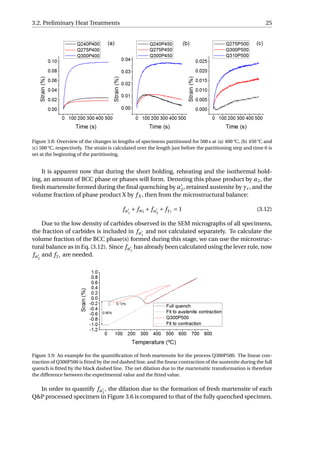
the optimal QT determined by experiments is higher than the calculated one. The changes
of experimental RA fraction with QT is also less sharp compared to the calculated results,
implying that QT can be selected from a wider range to obtain desired RA fraction. When
PT is chosen properly (400 °C in this study), the carbides precipitation is limited, and within
the chosen QT range (230−300 °C), RA fraction increases with increasing QT.
The partitioning time tp influences the carbon enrichment in austenite. Carbon en-
richment in austenite can be increased with increasing tp. If partitioning time is chosen
properly, austenite can be enriched to a level where no fresh martensite will form during
the final quenching. A further increase in tp results in more carbon in austenite until the
carbon content is stabilised, accompanied by a slight decrease in austenite fraction. This
will be reflected as an increasing RA fraction with tp followed by a slight decrease, which has
been observed in the second dilatometry tests: RA fraction increases until tp = 300 s, fol-
lowed by a slight decrease at tp = 500 s. After the stabilisation of carbon content in austen-
ite, any further increase in tp would lead to further consumption of austenite, resulting in
less RA fraction.
Figure 4.1: A summary of the volume fraction of RA obtained with different QTs. The results of obtained by
the dilatometry tests are labelled by DIL. For the preliminary heat treatments where the partitioning time
all equals to 500 s, the partitioning temperature is added after DIL. For the second set of dilatometry tests
where the partitioning is performed at 400 °C, the partitioning time tp is added after DIL. The synchrotron
XRD experiments are labelled by SXRD P400. The two arrows highlight RA fraction behaviour with increasing
partitioning time for QT = 300 °C and PT = 400 °C. The experimental results are compared with the calculated
results (CALC) using the methodology in literature [12].
Another important parameter is the heating rate during reheating. Lower heating rate
would mean longer interval between the initial quenching and partitioning step, and as
shown by our results, fast phase transformation and carbon enrichment can occur during
this stage. However, since all the heating rate is selected to be 5 °C/s in this work, it is not
known how the heating rate would influence the phase transformations during this stage.](https://image.slidesharecdn.com/8b2ffde7-c0f3-47a7-8f34-df7c41853fc3-170201023600/85/MasterThesis-YimingHu-57-320.jpg)
![50 4. Discussions
4.4. Comparison to Other Processes
In this work, the microstructure consisting of bainite, martensite and retained austen-
ite is obtained through the Q&P process. This microstructure mixture is conventionally
obtained through the austempering process, an example of which is shown by the temper-
ature vs. time diagram (Figure 4.2), where the fully austenitised steel is firstly quenched
to a temperature within the bainitic temperature range, followed by an isothermal holding
at this temperature and then a final quenching. Compared to the austempering process,
the kinetics of bainite formation during the Q&P process is much faster due to the accel-
erating effect of primary martensite on the bainitic transformation [74, 75]. For a direct
comparison, the strain vs. time diagram of a steel of the same composition as in Table 2.1
austempered at 400 °C is shown in Figure 4.2. There is a incubation time of about 30 s for
the bainite formation, and then it takes more than 1000 s to complete the phase transfor-
mation, which is marked by the plateau in the figure. The bainitic reaction in Q&P process
with a PT=400 °C takes 200−500 s to approach the completion, which is much less than the
time required for the austempering process. Apart from the time that can be saved during
heat treatment, the RA fraction can be adjusted in a wider range without formation of fresh
martensite, resulting in a microstructure consisting of tempered martensite, bainite and
retained austenite. In this study, RA fraction can be adjusted from 6.9 vol.% to 13.6 vol.%
without forming fresh martensite. By contrast, in the case of austempering, fresh marten-
site would even form during the final quenching with the completion of bainite transfor-
mation, depending on the chemical composition of the steel.
Figure 4.2: An example of the austempering process and the strain vs. time diagram of the studied specimen
processed with austempering. The inset shows an enlarged image of the dashed-square area.
The bainite/martensite multi-phase steels obtained through Q&P also show improved
mechanical properties. Gao et al. [76] obtained a low-carbon steel that exhibits a fatigue
limit of 770 MPa in the very high cycle fatigue regime and a tensile strength of 1410 MPa by a
Q&P-tempering process that obtained bainite during the initial quenching. Luo et al. [77]](https://image.slidesharecdn.com/8b2ffde7-c0f3-47a7-8f34-df7c41853fc3-170201023600/85/MasterThesis-YimingHu-58-320.jpg)
![4.4. Comparison to Other Processes 51
obtained the multi-phase steel that has a tensile strength of 1923 MPa and total elonga-
tion of 18.3%. Huang et al. [78] showed a significantly improved impact toughness from
84 J/cm2
for austempering to 104 J/cm2
for the Q&P heat treatment. The reported improve-
ment upon fatigue behaviour, strengths, ductility and toughness would be beneficial for
industrial applications. The obtained multi-phase steel in this study can be further charac-
terized mechanically in order to study the effect of different microstructures (e.g. different
RA volume fraction) on the mechanical behaviour.](https://image.slidesharecdn.com/8b2ffde7-c0f3-47a7-8f34-df7c41853fc3-170201023600/85/MasterThesis-YimingHu-59-320.jpg)

![Bibliography
[1] N. Fonstein, Advanced High Strength Sheet Steels: Physical Metallurgy, Design, Process-
ing, and Properties (Springer, 2015).
[2] S. Hayami and T. Furukawa, A family of high-strength cold-rolled steels, in Union Car-
bide Corporation (1975) p. 311.
[3] J. Hall, Evolution of advanced high strength steels in automotive applications, Presen-
tation at Joint Policy Council, Auto/Steel Partnership 18 (2011).
[4] R. Kuziak, R. Kawalla, and S. Waengler, Advanced high strength steels for automotive
industry, Archives of Civil and Mechanical Engineering 8, 103 (2008).
[5] M. Takahashi, Development of high strength steels for automobiles, Shinnittetsu Giho ,
2 (2003).
[6] D. K. Matlock and J. G. Speer, Third generation of AHSS: microstructure design con-
cepts, in Microstructure and texture in steels (Springer, 2009) pp. 185–205.
[7] D. K. Matlock and J. G. Speer, Design considerations for the next generation of advanced
high strength sheet steels, in Proceedings of 3rd International Conference on Structural
Steels (2006) pp. 774–781.
[8] A. F. L. Mark, Microstructural effects on the stability of retained austenite in transfor-
mation induced plasticity steels (2008).
[9] J. G. Speer, D. K. Matlock, B. C. de Cooman, and J. G. Schroth, Carbon partitioning into
austenite after martensite transformation, Acta Materialia 51, 2611 (2003).
[10] D. K. Matlock, V. E. Bräutigam, and J. G. Speer, Application of the quenching and parti-
tioning (Q&P) process to a medium-carbon, high-Si microalloyed bar steel, in Materials
Science Forum, Vol. 426 (Trans Tech Publ, 2003) pp. 1089–1094.
[11] J. G. Speer, F. C. R. Assunção, D. K. Matlock, and D. V. Edmonds, The "quenching
and partitioning" process: background and recent progress, Materials Research 8, 417
(2005).
[12] J. G. Speer, D. V. Edmonds, F. C. Rizzo, and D. K. Matlock, Partitioning of carbon from
supersaturated plates of ferrite, with application to steel processing and fundamentals
of the bainite transformation, Current Opinion in Solid State and Materials Science 8,
219 (2004).
[13] J. G. Speer, D. K. Matlock, B. C. de Cooman, and J. G. Schroth, Comments on “On the
definitions of paraequilibrium and orthoequilibrium”, Scripta Materialia 52, 83 (2005).
55](https://image.slidesharecdn.com/8b2ffde7-c0f3-47a7-8f34-df7c41853fc3-170201023600/85/MasterThesis-YimingHu-63-320.jpg)
![56 Bibliography
[14] M. Hillert and J. Ågren, On the definitions of paraequilibrium and orthoequilibrium,
Scripta Materialia 50, 697 (2004).
[15] M. Hillert and J. Ågren, Reply to comments on “on the definition of paraequilibrium
and orthoequilibrium”, Scripta Materialia 52, 87 (2005).
[16] N. Zhong, X. Wang, Y. Rong, and L. Wang, Interface migration between martensite and
austenite during quenching and partitioning (Q&P) process, Journal of Materials Sci-
ence and Technology 22, 751 (2006).
[17] J. G. Speer, R. E. Hackenberg, B. C. de Cooman, and D. K. Matlock, Influence of inter-
face migration during annealing of martensite/austenite mixtures, Philosophical Mag-
azine Letters 87, 379 (2007).
[18] M. J. Santofimia, L. Zhao, and J. Sietsma, Model for the interaction between interface
migration and carbon diffusion during annealing of martensite–austenite microstruc-
tures in steels, Scripta Materialia 59, 159 (2008).
[19] M. J. Santofimia, J. G. Speer, A. J. Clarke, L. Zhao, and J. Sietsma, Influence of interface
mobility on the evolution of austenite–martensite grain assemblies during annealing,
Acta Materialia 57, 4548 (2009).
[20] D. de Knijf, M. J. Santofimia, H. Shi, V. Bliznuk, C. Föjer, R. Petrov, and W. Xu, In
situ austenite–martensite interface mobility study during annealing, Acta Materialia
90, 161 (2015).
[21] H. Kawata, K. Hayashi, N. Sugiura, N. Yoshinaga, and M. Takahashi, Effect of marten-
site in initial structure on bainite transformation, in Materials Science Forum, Vol. 638
(Trans Tech Publ, 2010) pp. 3307–3312.
[22] K. Seto and H. Matsuda, Application of nanoengineering to research and development
and production of high strength steel sheets, Materials Science and Technology 29, 1158
(2013).
[23] J. Sun and H. Yu, Microstructure development and mechanical properties of quenching
and partitioning (Q&P) steel and an incorporation of hot-dipping galvanization during
q&p process, Materials Science and Engineering: A 586, 100 (2013).
[24] H. K. D. H. Bhadeshia and R. W. K. Honeycombe, Steels: microstructure and properties
(Butterworth-Heinemann, 2011).
[25] Y. Toji, G. Miyamoto, and D. Raabe, Carbon partitioning during quenching and parti-
tioning heat treatment accompanied by carbide precipitation, Acta Materialia 86, 137
(2015).
[26] J. G. Speer, E. de Moor, and A. J. Clarke, Critical assessment 7: quenching and parti-
tioning, Materials Science and Technology 31, 3 (2015).
[27] A. Navarro-López, J. Sietsma, and M. J. Santofimia, Effect of prior athermal martensite
on the isothermal transformation kinetics below Ms in a low-C high-Si steel, Metallur-
gical and Materials Transactions A 47, 1028 (2016).](https://image.slidesharecdn.com/8b2ffde7-c0f3-47a7-8f34-df7c41853fc3-170201023600/85/MasterThesis-YimingHu-64-320.jpg)
![Bibliography 57
[28] B. C. de Cooman, Structure–properties relationship in TRIP steels containing carbide-
free bainite, Current Opinion in Solid State and Materials Science 8, 285 (2004).
[29] S.-J. Kim, C. G. Lee, I. Choi, and S. Lee, Effects of heat treatment and alloying elements
on the microstructures and mechanical properties of 0.15 wt pct C transformation-
induced plasticity-aided cold-rolled steel sheets, Metallurgical and Materials Transac-
tions A 32, 505 (2001).
[30] C. García de Andrés, F. G. Caballero, C. Capdevila, and L. F. Álvarez, Application of
dilatometric analysis to the study of solid–solid phase transformations in steels, Mate-
rials Characterization 48, 101 (2002).
[31] G. L. Fisher and R. H. Geils, A method for obtaining quantitative dilatometric data from
alloys undergoing a phase transformation, Metallography 3, 229 (1970).
[32] T. A. Kop, A dilatometric study of the austenite/ferrite interface mobility (Delft Univer-
sity of Technology, 2000).
[33] H. S. Yang and H. K. D. H. Bhadeshia, Uncertainties in dilatometric determination of
martensite start temperature, Materials Science and Technology 23, 556 (2007).
[34] B. D. Cullity, Elements of x-ray diffraction, (1956).
[35] P. Suwanpinij, The synchrotron radiation for steel research, Advances in Materials Sci-
ence and Engineering 2016 (2016).
[36] J. A. Bearden, X-ray wavelengths, Reviews of Modern Physics 39, 78 (1967).
[37] H. Rietveld, A profile refinement method for nuclear and magnetic structures, Journal
of applied Crystallography 2, 65 (1969).
[38] L. Lutterotti, S. Matthies, H.-R. Wenk, A. S. Schultz, and J. W. Richardson Jr, Com-
bined texture and structure analysis of deformed limestone from time-of-flight neutron
diffraction spectra, Journal of Applied Physics 81, 594 (1997).
[39] D. Carmele, T. Rieger, K. Herrmann, S. Meyer, T. Lippmann, A. Stark, W. Bleck, and
U. Klemradt, Very hard synchrotron X-ray radiation as an advanced characterization
method applied to advanced high-strength steels, in Advanced Materials Research, Vol.
409 (Trans Tech Publications, 2012) pp. 660–665.
[40] B. B. He, U. Preckwinkel, and K. L. Smith, Fundamentals of two-dimensional X-ray
diffraction (XRD2
), Advances in X-ray Analysis 43, 273 (2000).
[41] A. Hammersley, Fit2d v9. 129 reference manual v3. 1, Inter Rep ESRF98HA01, ESRF,
Grenoble (1998).
[42] A. P. Hammersley, S. O. Svensson, M. Hanfland, A. N. Fitch, and D. Hausermann, Two-
dimensional detector software: from real detector to idealised image or two-theta scan,
International Journal of High Pressure Research 14, 235 (1996).
[43] A. P. Hammersley, Fit2d: an introduction and overview, European Synchrotron Radia-
tion Facility Internal Report ESRF97HA02T 68 (1997).](https://image.slidesharecdn.com/8b2ffde7-c0f3-47a7-8f34-df7c41853fc3-170201023600/85/MasterThesis-YimingHu-65-320.jpg)
![58 Bibliography
[44] W. David, Powder diffraction: least-squares and beyond, Journal of Research of the Na-
tional Institute of Standards and Technology 109, 107 (2004).
[45] M. I. A. Lourakis, A brief description of the Levenberg-Marquardt algorithm imple-
mented by levmar, Foundation of Research and Technology 4, 1 (2005).
[46] H. Gavin, The Levenberg-Marquardt method for nonlinear least squares curve-fitting
problems, (2011).
[47] B. H. Toby, R factors in Rietveld analysis: How good is good enough? Powder diffraction
21, 67 (2006).
[48] L. Lutterotti, Introduction to diffraction and the Rietveld
method, http://www.ccp14.ac.uk/ccp/web-mirrors/lutterotti/ lut-
tero/laboratoriomateriali/Rietveld.pdf, accessed: 2016-07-30.
[49] K. W. Andrews, Empirical formulae for the calculation of some transformation temper-
atures, Journal of the Iron and Steel Institute 207, 721 (1965).
[50] A. A. Gorni, Steel forming and heat treating handbook, Sao Vicente (2011).
[51] S. M. C. van Bohemen and J. Sietsma, Martensite formation in partially and fully
austenitic plain carbon steels, Metallurgical and Materials Transactions A 40, 1059
(2009).
[52] Y. K. Lee, Empirical formula of isothermal bainite start temperature of steels, Journal of
Materials Science Letters 21, 1253 (2002).
[53] H. K. D. H. Bhadeshia, Bulk nanocrystalline steel, Ironmaking & Steelmaking (2013).
[54] D. P. Koistinen and R. E. Marburger, A general equation prescribing the extent of
the austenite-martensite transformation in pure iron-carbon alloys and plain carbon
steels, Acta Metallurgica 7, 59 (1959).
[55] A. J. Clarke, J. G. Speer, D. K. Matlock, F. C. Rizzo, D. V. Edmonds, and M. J. Santofimia,
Influence of carbon partitioning kinetics on final austenite fraction during quenching
and partitioning, Scripta Materialia 61, 149 (2009).
[56] N. H. van Dijk, A. M. Butt, L. Zhao, J. Sietsma, S. E. Offerman, J. P. Wright, and S. van der
Zwaag, Thermal stability of retained austenite in trip steels studied by synchrotron x-ray
diffraction during cooling, Acta Materialia 53, 5439 (2005).
[57] R. E. Walpole, R. H. Myers, and S. L. Myers, Probability and statistics for engineers and
scientists, 9th ed., Vol. 5 (Prentice Hall, 2012).
[58] B. He, U. Preckwinkel, and K. L. Smith, Comparison between conventional and two-
dimensional XRD, Adv. X-Ray Anal 46, 37 (2003).
[59] N. Oku, K. Asakura, J. Inoue, and T. Koseki, In-situ observation of ferrite plate forma-
tion in low carbon steel during continuous cooling process, Journal of the Iron and Steel
Institute of Japan 94, B33 (2008).](https://image.slidesharecdn.com/8b2ffde7-c0f3-47a7-8f34-df7c41853fc3-170201023600/85/MasterThesis-YimingHu-66-320.jpg)
![Bibliography 59
[60] H. K. D. H. Bhadeshia, Widmanstätten ferrite, http://www.msm.cam.ac.uk/phase-
trans/2000/C9/lecture7.pdf, accessed: 2016-07-30.
[61] L. Cheng, A. Böttger, T. H. de Keijser, and E. J. Mittemeijer, Lattice parameters of iron-
carbon and iron-nitrogen martensites and austenites, Scripta metallurgica et materi-
alia 24, 509 (1990).
[62] Origin, The adjacent-averaging method, http://www.originlab.com/doc/Origin-
Help/Smooth-Algorithm, accessed: 2016-07-30.
[63] K.-i. Sugimoto, T. Iida, J. Sakaguchi, and T. Kashima, Retained austenite characteris-
tics and tensile properties in a TRIP type bainitic sheet steel. ISIJ international 40, 902
(2000).
[64] K.-i. Sugimoto, M. Murata, and S.-M. Song, Formability of Al-Nb bearing ultra high-
strength TRIP-aided sheet steels with bainitic ferrite and/or martensite matrix, ISIJ in-
ternational 50, 162 (2010).
[65] Y. H. Jiang, R. F. Zhou, D. Lu, and Z. H. Li, Microstructures and properties of a bainite
and martensite dual-phase cast steel fabricated by combination of alloying and con-
trolled cooling heat treatment, in Materials Science Forum, Vol. 475 (Trans Tech Publ,
2005) pp. 93–96.
[66] S. Van Bohemen, M. Santofimia, and J. Sietsma, Experimental evidence for bainite
formation below m s in fe–0.66 c, Scripta Materialia 58, 488 (2008).
[67] J.-C. Hell, M. Dehmas, S. Allain, J. M. Prado, A. Hazotte, and J.-P. Chateau,
Microstructure-properties relationships in carbide-free bainitic steels, ISIJ international
51, 1724 (2011).
[68] I. Yakubtsov and G. Purdy, Analyses of transformation kinetics of carbide-free bainite
above and below the athermal martensite-start temperature, Metallurgical and Mate-
rials Transactions A 43, 437 (2012).
[69] D. H. Kim, J. G. Speer, and B. C. De Cooman, The isothermal transformation of low-
alloy low-C CMnSi steels below Ms, in Materials Science Forum, Vol. 654 (Trans Tech
Publ, 2010) pp. 98–101.
[70] E. P. da Silva, D. de Knijf, W. Xu, C. Föjer, Y. Houbaert, J. Sietsma, and R. Petrov, Isother-
mal transformations in advanced high strength steels below martensite start tempera-
ture, Materials Science and Technology 31, 808 (2015).
[71] M. Oka and H. Okamoto, Swing back in kinetics near Ms in hypereutectoid steels, Met-
allurgical Transactions A 19, 447 (1988).
[72] D. Kim, J. G. Speer, and B. De Cooman, Isothermal transformation of a CMnSi steel
below the Ms temperature, Metallurgical and Materials Transactions A 42, 1575 (2011).
[73] D. Kim, S.-J. Lee, and B. C. De Cooman, Microstructure of low C steel isothermally
transformed in the Ms to Mf temperature range, Metallurgical and Materials Transac-
tions A 43, 4967 (2012).](https://image.slidesharecdn.com/8b2ffde7-c0f3-47a7-8f34-df7c41853fc3-170201023600/85/MasterThesis-YimingHu-67-320.jpg)
![60 Bibliography
[74] M. J. Santofimia Navarro, D. Hanlon, J. Sietsma, and S. van Bohemen, Perspectives
in high strength steels: interactions between non-equilibrium phases, in Proceedings of
the 2013 International Symposium on New Developments in Advanced High-Strength
Sheet Steels., edited by K. D. Hickey and R. E. Ashburn (Association for Iron & Steel
Technology, 2013) pp. 331–339.
[75] M. Santofimia, S. van Bohemen, and J. Sietsma, Combining bainite and martensite
in steel microstructures for light weight applications, Journal of the Southern African
Institute of Mining and Metallurgy 113, 143 (2013).
[76] G. Gao, B. Zhang, C. Cheng, P. Zhao, H. Zhang, and B. Bai, Very high cycle fatigue
behaviors of bainite/martensite multiphase steel treated by quenching-partitioning-
tempering process, International Journal of Fatigue 92, Part 1, 203 (2016).
[77] P. Luo, G. Gao, H. Zhang, Z. Tan, R. Misra, and B. Bai, On structure-property relation-
ship in nanostructured bainitic steel subjected to the quenching and partitioning pro-
cess, Materials Science and Engineering: A 661, 1 (2016).
[78] X. Huang, W. Liu, Y. Huang, H. Chen, and W. Huang, Effect of a quenching–long par-
titioning treatment on the microstructure and mechanical properties of a 0.2C bainitic
steel, Journal of Materials Processing Technology 222, 181 (2015).
[79] R. W. G. Wyckoff, Fluorite structure, Crystal Structures 1, 239 (1963).](https://image.slidesharecdn.com/8b2ffde7-c0f3-47a7-8f34-df7c41853fc3-170201023600/85/MasterThesis-YimingHu-68-320.jpg)
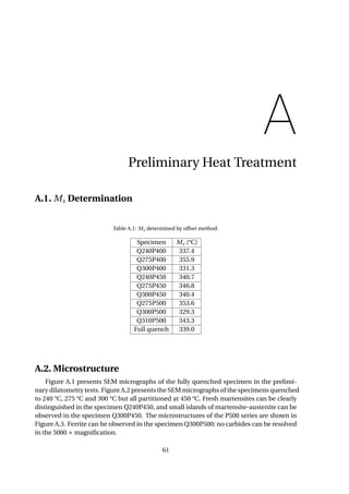
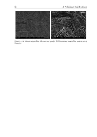
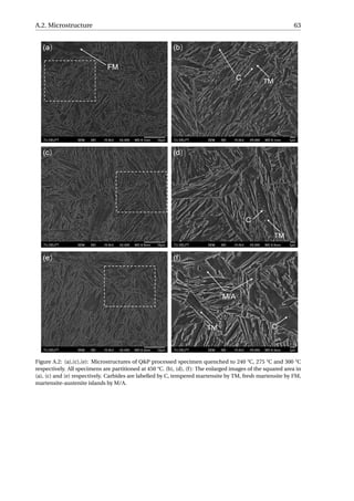
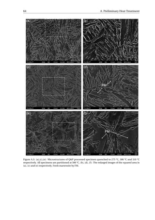
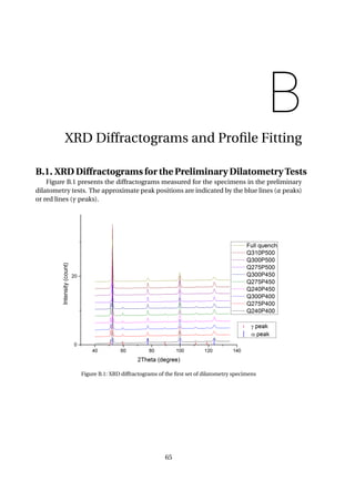
![66 B. XRD Diffractograms and Profile Fitting
B.2. In-situ XRD Experiments
The calibrated parameters are shown in Table B.1
Table B.1: Calibrated parameters for the in-situ XRD experiments.
Specimen
Refined beam
centre (mm,mm)
Refined sample
to detector
distance (mm)
Refined tilt plane
rotation angle (°)
Refined tilt angle
(°)
Full quench (50.653, 51.093) 301.709 17 0.058
Q230P400 (50.568, 51.113) 300.191 37.866 0.057
Q265P400 (50.684, 50.921) 300.447 38.807 -0.174
Q292P400 (50.652, 50.921) 300.883 22.213 0.091
The calibrated lattice parameters obtained for the calibrant CeO2 (aCeO2 ) and the litera-
ture value [79] are shown in Table B.2. Compared to the literature value, aCeO2 of Q265P400
deviates the most, and is smaller than the literature value. By checking the diffractogram of
CeO2 (Figure B.2, it is found that the apart from the CeO2 peaks, there are other peaks that
cannot be fitted, which implies that there is impurity in the CeO2 powder. This deviation
would result in a deviation of -0.26% in the determination of lattice parameter of austenite
(aγ) since aγ is calculated based on the calibration of CeO2. This deviation in aγ would lead
to a deviation of -0.20wt.% in the determination of carbon content.
Table B.2: Calibrated aCeO2 of the four specimens and aCeO2 from literature.
Specimen Full quench Q230P400 Q265P400 Q292P400 literature
aCeO2 (Å) 5.4135±0.0004 5.4146±0.0004 5.397±0.001 5.4147±0.0004 5.411
deviation (Å) 0.0025 0.0036 -0.014 0.0037 0
Figure B.2: Diffractogram of the calibrant CeO2 for the specimen Q265P400.
The Rwp values for the fitting of each XRD diffractogram obtained for different speci-
mens are shown in Figure B.3. The high Rwp values of the first few files are due to the spotty
rings observed in the corresponding 2D XRD profiles.](https://image.slidesharecdn.com/8b2ffde7-c0f3-47a7-8f34-df7c41853fc3-170201023600/85/MasterThesis-YimingHu-74-320.jpg)
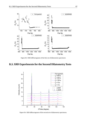

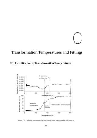
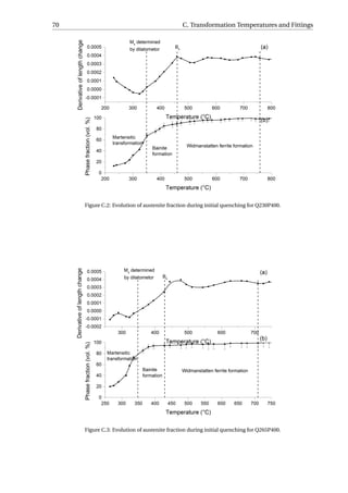
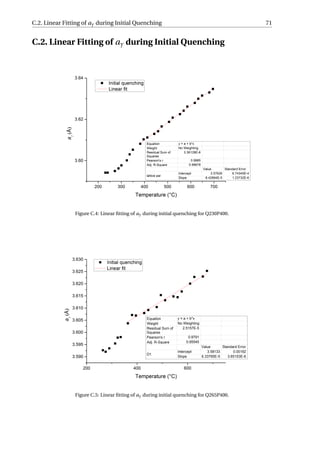
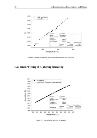
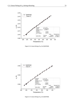
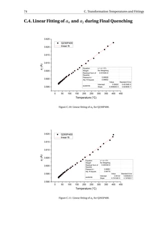
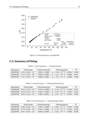


![[A. hobbacher] fatigue_design_of_welded_joints_and](https://cdn.slidesharecdn.com/ss_thumbnails/a-160512092007-thumbnail.jpg?width=640&height=640&fit=bounds)


